Sensitivity analysis of piezoelectric material parameters using Sobol indices
-
Franziska Anderl


Abstract
The applicability of the method of Sobol to the non-smooth, resonant behavior of a vibrational eigenmode of a piezoelectric element is examined. The goal is to quantify the sensitivity of the system upon variation of the piezoelectric material parameters. The randomly distributed piezoelectric material parameters needed for this statistical approach are taken from a Latin Hypercube Sampling (LHS). A hybrid computational approach is applied: The LHS process, the creation of the simulation model, the extraction of the resonance frequencies, and the calculation of the Sobol indices is performed in MATLAB®. The finite-element software COMSOL Multiphysics® is used for the computation of the electrical and mechanical properties of the considered block-shaped piezoceramic test specimen. To this end, an eigenfrequency analysis as well as a frequency domain study are set up, combined with a parametric sweep using the LHS parameter combinations as input. The convergence of the calculated Sobol indices depending on the LHS sampling size is investigated. It is shown that the Sobol analysis successfully identifies the most influential material parameters.
Zusammenfassung
Die Anwendbarkeit der Sobol Indizes auf das nicht-glatte, resonante Verhalten einer Schwingungseigenmode eines piezoelektrischen Elements wird mit dem Ziel untersucht, die Sensitivität des Systems bezüglich der Variation der piezoelektrischen Materialparameter zu quantifizieren. Die für diesen statistischen Ansatz benötigten, zufällig verteilten piezoelektrischen Materialparameter werden über ein Latin Hypercube Sampling (LHS) erzeugt. Ein hybrider Berechnungsansatz wird angewendet: Die Stichprobenerstellung, die Erstellung des Simulationsmodells, die Extraktion der Resonanzfrequenzen und die Berechnung der Sobol-Indizes werden in MATLAB® durchgeführt. Die Finite-Elemente Software COMSOL Multiphysics® wird zur Berechnung der elektrischen und mechanischen Eigenschaften des betrachteten blockförmigen, piezokeramischen Prüfkörpers verwendet. Zu diesem Zweck werden sowohl eine Eigenfrequenzanalyse als auch eine Frequenzraumstudie durchgeführt, wobei die Materialparameterkombinationen gemäß der erzeugten Stichprobe variiert werden. Die Konvergenz der berechneten Sobol-Indizes in Abhängigkeit der LHS-Stichprobengröße wird untersucht. Es zeigt sich, dass die Sobol-Analyse erfolgreich die einflussreichsten Materialparameter identifiziert.
1 Introduction
For the finite-element simulation of piezoelectric devices, material parameters are key to get reliable results. Consequently multiple techniques have been introduced to extract those parameters. The IEEE Standard on Piezoelectricity [1] suggests to use a number of specifically shaped test specimen that show isolated, monomodal vibrations. With help of measurements of the impedance curve, the material parameters can be calculated using analytic formulas. To determine the whole set of material parameters, at least four different test specimen are needed, which is costly, time-consuming and susceptible to errors [2]. Therefore in Ref. [3] a different approach using only two specimens in combination with an inverse determination procedure is presented. Others aim to identify all parameters using just one geometry with a high sensitivity to all material parameters at once [4] or use three test specimens of different shape or polarization [5]. In the literature, it is not quite clear how many different test specimens of different geometries are needed to identify the whole set of material parameters at once. For many applications that use a certain specimen geometry, only a subset of the material parameters is relevant. For the inverse method, an optimization routine is used to minimize the deviation between a measured and a simulated electrical impedance curve by varying the material parameters in the simulation. For this approach, a high sensitivity of the test specimen to all material parameters is needed. Knowing the sensitivity beforehand can thus greatly improve the material parameter determination process. One established way of expressing sensitivity quantitatively in the form of a measure is to calculate Sobol indices [6], [7], [8], [9]. In this work, the sensitivity of the resonance frequency of an exemplary block-shaped test specimen towards a variation of the piezoelectric material parameters is examined by means of Sobol’s method.
The calculation of Sobol indices is a statistical method, which means, that many randomly generated model values are required for a meaningful calculation. These are taken from a Latin Hypercube Sampling (LHS) of independently varied piezoelectric material parameters [10]. Within this study, for each such sampling point an eigenfrequency study and a frequency domain study are performed and compared. By means of the resonance frequencies, the Sobol indices of the selected piezoelectric material parameters are finally calculated.
The paper is structured as follows. The theory section provides a brief overview on the physics of piezoelectricity and the method of Sobol, which are both essential for this contribution. Subsequently, the computational model is introduced: The key differences of the eigenfrequency study and the frequency domain study are emphasized. The structure of the simulation model is outlined as well as the computational approach, followed by the results and discussion. At last, a conclusion and outlook is provided.
2 Theoretical aspects
2.1 Piezoelectric materials
In piezoelectric materials the direct and inverse piezoelectric effect occurs [2], [11], [12]. Common piezoelectric materials such as barium titanate and lead zirconate titanate (PZT) possess a crystal structure which consists of positively and negatively charged ions [2]. The charge centers overlap in the absence of external influences. When a force is applied to such materials, the crystal structure deforms, the charge centers shift, and dipoles form (direct piezoelectric effect), resulting in a measurable voltage difference across the deformed geometry. Similarly, an applied voltage results in a deformation of the material (inverse piezoelectric effect). The quantitative relationship between the magnitude of the displacement and the magnitude of the voltage difference can, in the linear case, be described by two coupled state equations for the dielectric displacement (D m ) and the mechanical stress (T ij ), known as the stress-charge form,
where E
n
is the electric field and S
kl
the mechanical strain [2]. The material specific parameters are
with
For the transversely isotropic behavior from above, a reduced set of material parameters

Electrical impedance magnitude of the block-shaped specimen geometry of this study. Three different eigenmodes are highlighted, from which the leftmost at about 50 kHz is used (the so-called T1-L mode).
2.2 The method of Sobol
A sensitivity analysis provides information about the sensitivity of a model to variations in the model parameters. It helps to distinguish between influential and insignificant parameters. This can be useful, for example, to identify the critical control variables of the model. Different kinds of sensitivity analysis approaches exist: A local sensitivity measure gives information about the change of the model output when one input parameter is slightly changed in proximity to a fixed value [8]. A more global statement is possible when the whole parameter space is covered by varying all input parameters simultaneously [14], [15]. This can be achieved by using a sampling procedure, for example the LHS-sampling [10]. For global sensitivity analysis, different sensitivity measures are common. One example are the Sobol indices which relate the variance in the model output to the input parameters [8]. In this work, the resonance frequency acts as the model output y[x] and is calculated upon variation of the n model parameters x = x1, …, x n , namely, the piezoelectric material parameters. The resulting variance of the model output is then decomposed into the contributions attributable to the individual input parameters x i . The first order Sobol index (the so-called main effect) of parameter x i is defined as [6], [16], [17]
where
To calculate second or higher order interactions S ij , S ijk , …, one would have to calculate the resulting model variance when two or more input parameters are varied and subtract the variance of each parameter alone. The sum of all first order, second order, third order to kth order indices naturally equals 1 [18],
The calculation of higher order Sobol indices is computational demanding, therefore an alternative index, the total Sobol index, which is defined as
is often used [6], [16], [17]. The total Sobol index
Direct calculation of above Sobol indices by means of solving the variance integrals is not feasible. Instead, a statistical method based on quasi-Monte Carlo sampling is used, needing only
where
3 Simulation model and methods
This work focuses on vibrational eigenmodes of block-shaped test specimens of piezoelectric materials. The eigenmodes are characterized by an increased vibration at their respective resonance frequency. One way to identify the resonance frequencies is by using the electrical impedance curve (that is, the frequency dependence of the impedance) of a specific test specimen; see Figure 1 for an example. The resonances are found at the minima; the maxima belong to their respective antiresonances [12]. Computationally, the impedance curve is retrieved by means of a frequency domain study, which assumes a steady-state harmonic behavior at a given frequency [19]. Therefore, the frequency range of interest is covered by a set of discrete frequencies for which the impedance is computed – quite similar to the approach in an actual measurement. Within a post-processing step, the resonance frequency is identified by finding the minimal value in the set of the computed impedance values. The accuracy of its position (in terms of frequency) largely depends on the frequency sweep discretization. A quadratic interpolation using three points around the minimum is employed to improve on this limitation.
As an alternative to the above-mentioned frequency domain study, an eigenfrequency study directly provides the relevant information, namely, a resonance position which does not depend on any frequency resolution. It solves for the eigenmodes of the system, again in the frequency domain [19]. As in general many eigenmodes are found within such a study, one drawback of this approach can be the difficulty to extract the desired one. On the bright side, this approach offers a significantly smaller simulation time compared to a frequency sweep. In the present work, we focus on the eigenmode approach but also exemplary compare it to the results from a frequency domain study to ensure consistency.
3.1 COMSOL model
The aforementioned eigenfrequency and frequency domain studies are implemented in the finite-element software package COMSOL Multiphysics® [20]. For our analysis, a block of length 30 mm, width 10 mm, and thickness 2 mm is used. This is the same setup as can be found in Refs. [2], [3]. The block is polarized in the thickness direction (z-direction) and made of the material PIC255, a PZT-type piezoelectric ceramic for which optimized material parameters can be found in Ref. [3] and are reproduced in Table 1 for reference. Furthermore, as a loss and damping model, the loss factor damping is used, for which the tensors ϵ S and c E from Eqs. (1) and (2) are supplemented with an imaginary part, that represents a loss or damping factor, as follows [12]:
Material parameters for PIC255 in stress-charge form; material density is taken as ρ = 7,800 kg/m3 [3].
| Parameter | Unit | Value |
|---|---|---|
|
|
N/m2 | 12.46 ⋅ 1010 |
|
|
N/m2 | 7.86 ⋅ 1010 |
|
|
N/m2 | 8.06 ⋅ 1010 |
|
|
N/m2 | 12.06 ⋅ 1010 |
|
|
N/m2 | 2.04 ⋅ 1010 |
| e 31 | C/m2 | −6.86 |
| e 33 | C/m2 | 16.06 |
| e 15 | C/m2 | 11.90 |
|
|
F/m | 7.31 ⋅ 10−9 |
|
|
F/m | 6.81 ⋅ 10−9 |
As reference values for this work, an isotropic loss factor η s = 0.0129 for mechanical damping and an identical dielectric loss factor η ϵs = 0.0129 for the electrical permittivity are assumed [2]. In total, this yields n = 11 independent material parameters for this study.
In COMSOL Multiphysics® piezoelectricity is modeled via the Solid Mechanics and Electrostatics physics interfaces which are coupled via the Piezoelectricity Multiphysics interface using the piezoelectric material model and the piezoelectric charge conservation nodes. As boundary conditions a voltage terminal of magnitude 1 V is applied to the top surface of the block-shaped geometry while the bottom one is grounded. Two symmetry planes are implemented to reduce the computational costs; see Figure 2. In the same figure, the mesh is visualized: a cubic mesh consisting of 15 × 5 × 5 elements is chosen.

Model geometry and mesh of the block-shaped test specimen considered in this work. Highlighted are the symmetry planes used to reduce the model size.
For the frequency domain study, frequencies in the range of 35–65 kHz in steps of 0.5 kHz are selected. The choice of this frequency range is such that the zeroth order T1-L transverse mode in the length (x-)direction is excited. As can be seen in Figure 1, this resonance is particularly suitable for this study as it is nicely separated from other, overlapping resonances. Accordingly, the eigenfrequency study in COMSOL Multiphysics® is configured to search for eigenvalues around 40 kHz which is below this resonance. Together with an algorithm setting to only compute eigenmodes with real part larger than the provided frequency value, this ensures that the resonance instead of the antiresonance frequency is identified.
3.2 Computational approach
The LHS sampling as well as the COMSOL Multiphysics® model creation are performed using MATLAB® and the COMSOL LiveLink™ for MATLAB®, followed by the simulation using COMSOL Multiphysics®. The post-processing and statistical evaluation are again carried out in MATLAB®.
Within this study, the material parameters are sampled in a 5 % interval from the literature values provided in Table 1 using the lhsdesign() function of MATLAB®. Sample sizes up to m = 15,000 are realized. Therefore, a plain, sequential parametric sweep is not an ideal choice. Even an optimistically short single simulation duration of 1 min (for the frequency domain study) would yield a total runtime of about seven weeks; similarly the eigenfrequency study would still take over 70 h. Luckily, the single model evaluation is computationally rather cheap. Therefore, the concept of task parallelism via the batch sweep functionality of COMSOL Multiphysics® is used: the total parameter sweep is distributed among many physical CPU cores (32 in our case), each process using just a single core. Interestingly, even spreading over twice as many logical CPU cores via simultaneous multithreading works quite well, speeding up the simulations further. This reduces the calculation time by orders of magnitudes to only days and hours instead of weeks and days, respectively.
As an example, Figure 3 shows the distribution of the resonance frequencies for the eigenfrequency study using a sample size of m = 15,000. The reference resonance frequency using the literature material parameters from Table 1 is indicated as well.

Distribution of the resonance frequencies for the eigenfrequency study using a sample size of m = 15,000, resulting in (n + 2) ⋅ m = 195,000 resonance positions in total.
4 Results and discussion
Since the Sobol indices are a statistical measure, adequate amounts of data have to be included in their calculation to obtain reliable values, depending on the problem’s complexity. To assert a convergence, different sample sizes, ranging from m = 100 to m = 15,000 were generated and the Sobol indices were calculated according to Eqs. (6) and (7). Due to the large computational effort of the frequency domain study, the last sample size was only carried out for the eigenfrequency study. The following results refer to the eigenfrequency analysis.
For small sample sizes m, a statistically sufficient sampling of the parameter space is not given and large variations between different realizations of the random LHS process for identical, but small m are to be expected. This is accounted for by creating multiple LHS samples while varying the random seed at fixed sample size m. For the smallest sample size m = 100, twenty samplings were created, for m = 1,000 and m = 15,000 ten samplings were sufficient, as the spread of the resulting Sobol indices decreased rapidly. In Figure 4 the convergence of the Sobol indices as function of the sample size m is indicated in terms of the mean value together with the 95 % confidence interval of these samplings. When comparing the mean value of all indices for the smallest sample size (m = 100) with the largest sample size (m = 15,000), one notices that the value varies only slightly. However, the confidence interval is very large for the smallest sample size (m = 100) compared to the largest sample size (m = 15,000). This offers an alternative approach for calculating the Sobol indices. Instead of increasing the sample size, the number of samplings for a smaller sample size could be increased. In this way, the calculation time is decreased and an estimate of the Sobol indices is available early in the process. Hence, our results indicate that the mean value of a statistical ensemble of Sobol indices for a small sample size provides a better estimation of its true value than a single Sobol index for a large sample size. This becomes particularly relevant in the case of limited computational resources and/or time.

Evolution of Sobol indices with sample size: (a) First order and (b) total Sobol indices, respectively, for the most influential material parameters as a function of sample size. The points indicate the mean value from multiple realizations of the random LHS sampling; the bands correspond to the respective 95 % confidence interval.
Table 2 provides the mean Sobol indices for a sample size of m = 15,000. The first four material parameters
First order and total Sobol index for the sensitivity of the position of the T1-L mode of a block shaped test specimen on its piezoelectric material parameter values; PIC255 is used as reference, see Table 1. The Sobol index values refer to the mean value from multiple realizations of the random LHS sampling of size m = 15,000; the 95 % confidence interval of their resulting statistical distribution is provided as well. The slope in the last column indicates the direction and magnitude of the shift of the resonance frequency found in Figure 5.
| Material parameter | First order Sobol ind. | Conf. interval | Total Sobol ind. | Conf. interval | Slope in kHz/% |
|---|---|---|---|---|---|
|
|
0.7786 | 0.0088 | 0.7766 | 0.0038 | 0.536 |
|
|
0.1375 | 0.0075 | 0.1366 | 0.0013 | −0.225 |
|
|
0.0611 | 0.0092 | 0.0689 | 0.0005 | −0.157 |
|
|
0.0208 | 0.0081 | 0.01784 | 0.0001 | 0.078 |
|
|
1.8 ⋅ 10−10 | 9.1 ⋅ 10−11 | 5.0 ⋅ 10−17 | 3.2 ⋅ 10−19 | – |
|
|
−2.0 ⋅ 10−11 | 3.3 ⋅ 10−11 | 2.1 ⋅ 10−19 | 1.5 ⋅ 10−20 | – |
|
|
1.8 ⋅ 10−9 | 8.7 ⋅ 10−9 | 2.0 ⋅ 10−14 | 1.3 ⋅ 10−16 | – |
| e 31 | 1.0 ⋅ 10−9 | 4.3 ⋅ 10−9 | 8.5 ⋅ 10−15 | 8.0 ⋅ 10−17 | – |
| e 33 | 1.3 ⋅ 10−8 | 1.2 ⋅ 10−8 | 3.5 ⋅ 10−14 | 2.0 ⋅ 10−16 | – |
| e 15 | 3.7 ⋅ 10−11 | 1.3 ⋅ 10−10 | 2.2 ⋅ 10−17 | 1.3 ⋅ 10−19 | – |
| η | 7.6 ⋅ 10−8 | 5.0 ⋅ 10−7 | 4.0 ⋅ 10−9 | 3.0 ⋅ 10−11 | – |
As the first order Sobol index and total Sobol index show almost the same value, no interaction exist between the material parameters. In the following, only the parameters
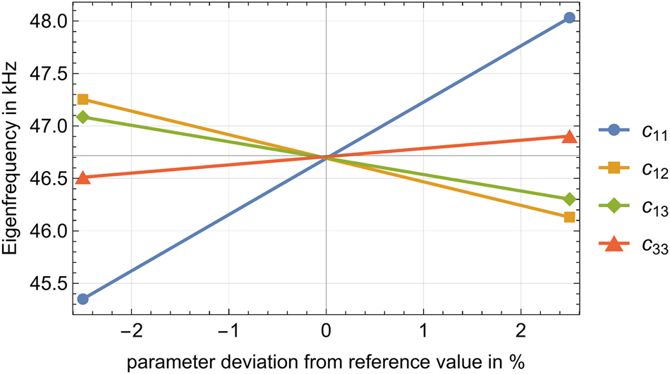
Shift of the resonance frequency when each of the given material parameter is varied separately around its literature value. The slope is another measure for the sensitivity of the resonance position with respect to this parameter.
When comparing the first order Sobol index and total Sobol index, one might notice that the total Sobol index is slightly smaller than the first order one. However, when inspecting Table 2 more closely, one finds that the confidence intervals of both indices overlap. Moreover, the raw data shows this behavior not in general: there are cases where the total Sobol is indeed larger than the first order one. In Figure 6 this is exemplified for Sobol indices of the

Comparison of the first order and total Sobol index for the
For the calculation of the Sobol indices, an eigenfrequency study was used, as this study type offers computational advantages. A frequency domain study as described in Subsection 3.2 should yield the same results. Accordingly, Table 3 shows this consistency between these two study types by comparing the respective Sobol indices for an identical LHS sampling of size m = 10,000. The remaining, small discrepancies we attribute to the limitation of the resonance position determination for the frequency domain study due to the finite frequency resolution in this study type.
Same as Table 2 but comparing the Sobol indices calculated by means of a frequency domain study and eigenfrequency study, respectively, using the same LHS sampling of size m = 10,000.
| Frequency domain study | Eigenfrequency study | |||
|---|---|---|---|---|
| Material parameter | First order Sobol ind. | Total Sobol ind. | First order Sobol ind. | Total Sobol ind. |
|
|
0.8075 | 0.7852 | 0.8086 | 0.7840 |
|
|
0.1599 | 0.1446 | 0.1623 | 0.1411 |
|
|
0.0734 | 0.0648 | 0.0766 | 0.0679 |
|
|
−0.0050 | 0.0172 | −0.0029 | 0.0179 |
5 Conclusion and outlook
In this work, the first order and total Sobol indices were investigated as a global sensitivity measure for piezoelectric material parameters. More specifically, a block-shaped test specimen and the position of one of its vibrational eigenmodes upon variation of the piezoelectric material parameters were analyzed. To this end, an eigenfrequency analysis was implemented using COMSOL Multiphysics®. For efficient computation, a batch sweep was applied to execute a large number of simulations simultaneously. As a sampling strategy for possible material parameter values, a Latin Hypercube Sampling (LHS) was used. For the sample generation and the later calculation of the Sobol indices, MATLAB® was utilized. To obtain reliable values, the sample size was increased until a converging behavior was found. In this context an alternative sampling approach was identified: At a parameter-screening level, faster convergence, i.e., less computational effort, was found when a statistical analysis of multiple Sobol analyses at relatively small sample size is performed.
For the specific example investigated in this work, four material parameters could be identified as most influential, which agrees with the qualitative expectation from other references [2], [3]. The first order and total Sobol indices of these material parameters showed similar magnitudes, which is a sign of no interaction between the material parameters.
In this work, a geometric shape and operating point resulting in an isolated resonance was considered. Next steps would be to use specimen geometries or frequency ranges that show also other, maybe overlapping vibrational modes. This would possibly include sensitivity interactions between the material parameters. The applicability of the described method needs to be tested for such cases.
A possible application of the Sobol analysis in the context of piezoelectric material parameter determination could be to act as an objective function in the design process of an optimized specimen geometry. The goal is to maximize the sensitivity to all parameters. This enhances the accuracy of the determined parameters and reduces the number of specimen needed for the determination process. For the design of the optimization process itself, a purely simulative approach, similar to this study, is certainly advantageous.
About the authors

M.Sc. Franziska Anderl studied Applied Math and Physics at the Technische Hochschule Nürnberg Georg Simon Ohm from 2019 to 2024 where she is now employed as a research assistant.

Michael Mayle graduated in physics from the University of Heidelberg and received a PhD degree in Quantum Physics in 2009 from the same university. This was followed by a post-doctoral phase at the University of Hamburg (2010) and, as part of a DAAD post-doctoral fellowship, at the JILA Institute, University of Colorado Boulder (2011–2012). At the beginning of 2023, Michael Mayle was appointed as a Professor of Applied Physics with focus on applied computational physics at the Faculty of Applied Mathematics, Physics and Humanities at the Technische Hochschule Nürnberg Georg Simon Ohm (Ohm). Previously he held R&D positions in industry where he gained extensive experience in application-oriented multiphysics simulation. In his new position at the Ohm, Michael Mayle is establishing a research group in the field of applied computational physics and is a member of the newly founded doctoral research center “Center for Physical and Biomedical Engineering”.
-
Research ethics: Not applicable.
-
Informed consent: Not applicable.
-
Author contributions: All authors have accepted responsibility for the entire content of this manuscript and approved its submission.
-
Use of Large Language Models, AI and Machine Learning Tools: None declared.
-
Conflict of interest: The authors state no conflict of interest.
-
Research funding: None declared.
-
Data availability: Not applicable.
References
[1] “Publication and proposed revision of ANSI/IEEE standard 176-1987, ANSI/IEEE standard on piezoelectricity,” IEEE Trans. Ultrason. Ferroelectrics Freq. Control, vol. 43, no. 5, 1996.10.1109/TUFFC.1996.535477Search in Google Scholar
[2] S. J. Rupitsch, Piezoelectric Sensors and Actuators: Fundamentals and Applications, Berlin, Springer, 2019.10.1007/978-3-662-57534-5Search in Google Scholar
[3] S. J. Rupitsch and J. Ilg, “Complete characterization of piezoceramic materials by means of two block-shaped test samples,” IEEE Trans. Ultrason. Ferroelectrics Freq. Control, vol. 62, no. 7, pp. 1403–1413, 2015, https://doi.org/10.1109/tuffc.2015.006997.Search in Google Scholar
[4] O. Friesen, L. Claes, C. Scheidemann, N. Feldmann, T. Hemsel, and B. Henning, “Estimation of temperature-dependent piezoelectric material parameters using ring-shaped specimens,” J. Phys.: Conf. Ser., vol. 2822, p. 012125, 2024, https://doi.org/10.1088/1742-6596/2822/1/012125.Search in Google Scholar
[5] T. Lahmer, M. Kaltenbacher, B. Kaltenbacher, R. Lerch, and E. Leder, “FEM-based determination of real and complex elastic, dielectric, and piezoelectric moduli in piezoceramic materials,” IEEE Trans. Ultrason. Ferroelectrics Freq. Control, vol. 55, no. 2, pp. 465–475, 2008. https://doi.org/10.1109/tuffc.2008.664.Search in Google Scholar
[6] C. Prieur and S. Tarantola, “Variance-based sensitivity analysis: theory and estimation algorithms,” in Handbook of Uncertainty Quantification, Cham, Springer International Publishing, 2016.10.1007/978-3-319-11259-6_35-1Search in Google Scholar
[7] F. Montomoli, Hrsg. Uncertainty Quantification in Computational Fluid Dynamics and Aircraft Engines, Cham, Springer International Publishing, 2019.10.1007/978-3-319-92943-9Search in Google Scholar
[8] B. Iooss and A. Saltelli, “Introduction to sensitivity analysis,” in Handbook of Uncertainty Quantification, Cham, Springer International Publishing, 2016.10.1007/978-3-319-11259-6_31-1Search in Google Scholar
[9] S. Brandstaeter, S. L. Fuchs, J. Biehler, R. C. Aydin, W. A. Wall, and C. J. Cyron, “Global sensitivity analysis of a homogenized constrained mixture model of arterial growth and remodeling,” J. Elast., vol. 145, no. 1, pp. 191–221, 2021. https://doi.org/10.1007/s10659-021-09833-9.Search in Google Scholar
[10] M. D. McKay, R. J. Beckman, and W. J. Conover, “A comparison of three methods for selecting values of input variables in the analysis of output from a computer code,” Technometrics, vol. 21, no. 2, p. 239–245, 1979. https://doi.org/10.1080/00401706.1979.10489755.Search in Google Scholar
[11] Q.-H. Qin, Advanced Mechanics of Piezoelectricity, Berlin, Heidelberg, Springer, 2013.10.1007/978-3-642-29767-0Search in Google Scholar
[12] K. Uchino, Applied Mathematics in Ferroelectricity and Piezoelectricity, Basel, MDPI, 2023.10.3390/books978-3-0365-1319-5Search in Google Scholar
[13] H. Altenbach, Kontinuumsmechanik: Einführung in die materialunabhängigen und materialabhängigen Gleichungen, Berlin, Heidelberg, Springer, 2018.10.1007/978-3-662-57504-8Search in Google Scholar
[14] A. Saltelli, Global Sensitivity Analysis: The Primer, Chichester, John Wiley, 2008.10.1002/9780470725184Search in Google Scholar
[15] M. T. Wentworth, R. C. Smith, and H. T. Banks, “Parameter selection and verification techniques based on global sensitivity analysis illustrated for an HIV model,” SIAM/ASA J. Uncertain. Quantif., vol. 4, no. 1, pp. 266–297, 2016. https://doi.org/10.1137/15m1008245.Search in Google Scholar
[16] S. Brandstäter, Global Sensitivity Analysis for Models of Active Biomechanical Systems, Ph.D. thesis, Technische Universität München, 2021.Search in Google Scholar
[17] I. M. Sobol, “Global sensitivity indices for nonlinear mathematical models and their Monte Carlo estimates,” Math. Comput. Simulat., vol. 55, no. 1, pp. 271–280, 2001. https://doi.org/10.1016/s0378-4754(00)00270-6.Search in Google Scholar
[18] A. Saltelli, P. Annoni, I. Azzini, F. Campolongo, M. Ratto, and S. Tarantola, “Variance based sensitivity analysis of model output. Design and estimator for the total sensitivity index,” Comput. Phys. Commun., vol. 181, no. 2, pp. 259–270, 2010. https://doi.org/10.1016/j.cpc.2009.09.018.Search in Google Scholar
[19] Structural Mechanics Module User’s Guide, “COMSOL Multiphysics® v. 6.2,” Stockholm, Sweden, COMSOL AB, 2024.Search in Google Scholar
[20] “COMSOL Multiphysics® v. 6.2,” Stockholm, Sweden, COMSOL AB. Available at: www.comsol.com.Search in Google Scholar
© 2025 the author(s), published by De Gruyter, Berlin/Boston
This work is licensed under the Creative Commons Attribution 4.0 International License.
Articles in the same Issue
- Frontmatter
- Editorial
- 6. Workshop ,,Messtechnische Anwendungen von Ultraschall“ vom 17. bis 19. Juni 2024 im Kloster Drübeck
- Research Articles Focus Section
- Estimation of piezoelectric material parameters of ring-shaped specimens
- Phased-Array basiertes Structural Health Monitoring zur Delaminationserkennung bei Mehrschichtsystemen
- Luftgekoppelter Ultraschall für die Prüfung des Alterungszustandes von Klebeverbindungen
- Sensitivity analysis of piezoelectric material parameters using Sobol indices
- Research Articles
- Investigations on anelastic effects in electrical discharge machined titan grade 2 flexures for the use in precision force instruments
- 2D image-based electrical contact surface degradation and its health assessment
- Review Article
- From marker features to multimodal fusion: a review of vision-based tactile sensor design and development