Investment Optimization in Insurance Portfolios: A Quantitative Analysis of Financial Services Authority of Indonesia Regulations
-
Nanang Susyanto
 ,
M. Haikal Sedayo
,
M. Haikal Sedayo

Abstract
This study examines investment optimization strategies for insurance company portfolios in Indonesia, focusing on the quantitative impacts of Financial Services Authority (OJK) Regulation No. 5 of 2023. The research evaluates how this regulation influences insurers’ asset allocation decisions and portfolio construction. Through financial modeling and statistical analysis, the study assesses changes in allowable assets, investment limits, and risk management requirements introduced by the regulation. Key areas of analysis include modifications to permitted investments, adjustments to maximum allocation limits, new requirements for investments in corporate bonds and medium-term notes, and revised affiliated party investment rules. The research aims to identify optimal portfolio compositions that maximize returns while adhering to the regulatory framework. Findings provide insights into effective investment strategies for Indonesian insurance companies operating under the current regulatory environment, with recommendations for optimizing portfolios to balance risk and return in compliance with OJK regulations. This paper is among the first to incorporate the latest OJK regulatory limits into a CVaR-based optimization framework, offering a practical approach for compliance-oriented asset management in the Indonesian insurance sector.
1 Introduction
Investment optimization in insurance portfolios is a critical area of study, aiming to balance risk and return while adhering to regulatory frameworks. The insurance industry faces unique challenges in portfolio management due to the need to match assets with liabilities, ensure solvency, and comply with stringent regulatory requirements. Regulation No. 5 of 2023, issued by the Financial Services Authority (OJK) in Indonesia, introduces new guidelines that significantly impact the investment strategies of insurance companies (Otoritas Jasa Keuangan (OJK) 2023).
The COVID-19 pandemic has exposed the limitations of traditional portfolio optimization methods, such as the Markowitz model (Markowitz 1952), which often fail to account for non-normally distributed returns and extreme market events. This has highlighted the need for more sophisticated models that can better manage risk and enhance portfolio resilience (Irhamni 2024). For instance, the Markowitz model and the Single Index Model, when applied to Indonesian stock portfolios, reveal the dynamic nature of financial markets and underscore the necessity of continuous portfolio monitoring and adaptation to maintain performance (Oktavianus Yusan and Riyadi 2024). A study on the LQ-45 stock index, government bonds, USD, gold, and Bitcoin underscores the importance of diversifying investment instruments to minimize risk and maximize returns. Notably, an optimal portfolio comprising 18 % Bitcoin and 82 % gold demonstrated a promising expected return with manageable risk (Semeru and Nainggolan 2023).
OJK regulations, both directly and indirectly, influence the performance of insurance companies. Previous studies (Chen and Hieber 2016; Gaganis, Hasan, and Pasiouras 2020; McShane, Cox, and Butler 2010; Subramanian and Wang 2021; Zhang and Cao 2023) have highlighted the significant impact of regulatory changes on the operations and financial performance of insurance firms. For instance, increased regulation often leads to higher operating costs, though it may also drive cost efficiencies (Cheng and Li 2018; Zhang and Cao 2023). The adaptability of insurance companies to regulatory changes varies by size: smaller firms may adapt more quickly due to their flexibility, while larger firms benefit from established management systems. Medium-sized companies often face greater challenges in adaptation (Armantier, Foncel, and Treich 2023). Moreover, regulatory constraints – particularly solvency requirements – play a crucial role in shaping the investment strategies of insurance companies by enforcing risk management practices that ensure financial stability (Zhang and Cao 2023).
While many international jurisdictions have established quantitative and qualitative constraints on insurance investments to improve solvency and resilience, Indonesia’s OJK regulation introduces a distinct set of thresholds that align with this global trend but reflect local market structures. The new regulations impose stringent limits on the types and proportions of investments that insurance companies can hold. For example, specific caps are placed on investments in corporate bonds, mutual funds, and real estate. Additionally, the regulations emphasize maintaining high solvency levels and implementing robust risk management practices. Insurance companies must ensure that their asset-liability management strategies effectively mitigate the risks associated with their investment portfolios. These investment limits are designed to encourage more prudent decision-making, factoring in the companies’ capital capacity to absorb associated risks. This research provides a foundation for quantitatively analyzing the impact of OJK Regulation No. 5 of 2023 on the investment strategies of Indonesian insurance companies.
In recent years, the Indonesian insurance sector has witnessed high-profile investment failures, notably the Jiwasraya and Asabri cases, which revealed significant weaknesses in asset allocation, risk oversight, and regulatory enforcement. Although not explicitly cited as a direct response, the issuance of OJK Regulation No. 5 of 2023 can be seen as part of a broader regulatory reform agenda aimed at preventing similar incidents.
While numerous studies have examined portfolio optimization using methods such as mean-variance analysis or the Single Index Model, these approaches often abstract away from real-world regulatory constraints that directly affect institutional investors such as insurance companies. Prior work has explored the impact of solvency regulations on investment behavior globally (Chen and Hieber 2016; Gaganis, Hasan, and Pasiouras 2020; McShane, Cox, and Butler 2010), and some studies have analyzed diversification strategies using alternative assets such as gold and Bitcoin (Semeru and Nainggolan 2023). However, there remains a significant gap in the literature regarding the quantitative evaluation of regulatory restrictions on portfolio construction in the Indonesian insurance sector. In particular, few studies have explicitly modeled how asset class limits and solvency constraints under OJK Regulation No. 5 of 2023 affect the structure and risk profile of optimized insurance portfolios. Moreover, from a methodological perspective, constrained optimization problems, such as those governed by regulatory investment limits, can benefit from insights into efficient estimation under equality constraints, as previously discussed by Susyanto and Klaassen (2017). This study aims to fill that gap by applying a Conditional Value-at-Risk (CVaR) optimization framework to Indonesian financial data, incorporating investment caps and rules outlined in the current regulatory regime. Unlike prior studies focusing predominantly on theoretical or international contexts, this research uniquely applies CVaR optimization within the explicit regulatory constraints set forth by OJK Regulation No.5 of 2023, providing actionable insights for the Indonesian insurance sector. The remainder of the paper is organized as follows: Section 2 presents our proposed method for quantitatively investigating the impact of OJK regulations on portfolio optimization. Section 3 discusses the results based on real data. Finally, Section 4 provides the conclusions.
2 Methods
OJK Regulation No.5 of 2023 introduces a comprehensive set of investment rules for insurers in Indonesia. The regulation’s objective is to ensure insurers maintain financial health by managing portfolio risks in line with solvency requirements. Key provisions of the regulation include: (a) updated definitions of permitted assets and counterparty limits, (b) exclusion of certain high-risk assets, (c) revised bases for asset valuation, (d) specific requirements for investments in instruments like corporate bonds, medium-term notes (MTN), repurchase agreements (REPO), and gold, (e) new maximum investment concentration limits, and (f) stricter reporting obligations (Otoritas Jasa Keuangan (OJK) 2023).
One notable aspect of these new rules is the introduction of maximum investment restrictions by OJK. Insurers are now subject to explicit caps on exposure to different asset classes and counterparties. These include, for example, a maximum of 20 % per bank for time deposits, 1 % per rural bank (BPR/BPRS) with a total cap of 5 %, and 50 % for certificates of deposit. Listed equity investments are limited to 10 % per issuer and 40 % in total, while corporate bonds are capped at 20 % per issuer and 50 % in total. The regulation also governs exposure to mutual funds, real estate investment trusts, repurchase agreements, and direct participation in non-listed companies, each with their respective limits. Investments in pure gold are limited to 10 % of total assets, and infrastructure funds are capped at 20 % in aggregate. Additional constraints apply to policy loans, land and buildings, foreign securities, and instruments issued by multinational or foreign institutions. Collectively, these limits are designed to enforce diversification, enhance solvency, and promote prudent risk management within insurance portfolios (Otoritas Jasa Keuangan (OJK) 2023).
These types of regulatory limits are not unique to Indonesia. From a comparative perspective, the investment constraints introduced by OJK Regulation No. 5 of 2023 reflect similar trends observed in international regulatory frameworks. For example, the Solvency II directive in the European Union mandates risk-based capital adequacy and prudent person principles, requiring insurers to ensure that investments are suitable and diversified (European Commission 2009). In the United States, the NAIC’s Model Investment Law establishes specific limits on asset classes and encourages risk-aware portfolio management (National Association of Insurance Commissioners 2021). Similarly, Singapore’s Monetary Authority imposes concentration limits and promotes asset-liability matching in insurance portfolios (Monetary Authority of Singapore 2020). The OJK regulation follows these global practices by introducing quantitative investment limits and emphasizing solvency, thus signaling Indonesia’s alignment with international efforts to enhance insurance sector resilience and transparency.
The changes introduced demonstrate a proactive approach to addressing the evolving challenges in the insurance sector. The regulation aims to enhance the stability and competitiveness of Indonesia’s insurance industry by refining rules, clarifying definitions, and adapting to new financial products and technologies. As suggested by Peng and Li (2023), in their study on optimal investment strategies with learning about return predictability, regulators and insurers must continually adapt to changing market conditions and emerging risks. The effectiveness of these new regulations in achieving their intended goals will require ongoing monitoring and possible future adjustments.
In this study, we focus on the investment constraints related to the proportion of stocks and bonds, investigating quantitatively how portfolios in the Indonesian insurance sector are impacted by the regulations set forth by the OJK (Otoritas Jasa Keuangan (OJK) 2023). Our methodology centers on the application of Conditional Value-at-Risk (CVaR) as a risk measure, building on the foundational work of Uryasev (2000) and Acerbi and Simonetti (2002) in portfolio optimization. CVaR, also known as Expected Shortfall, provides a more comprehensive assessment of tail risk compared to traditional Value-at-Risk (VaR) measures. It quantifies the expected loss when losses exceed the VaR threshold, offering a coherent risk measure that is particularly relevant in the context of insurance portfolios, where extreme events can have significant financial impacts. The CVaR approach is particularly suited for insurance portfolio due to its robust handling of tail risks, capturing severe loss scenarios better than traditional VaR measures. Given regulatory emphasis on solvency and stability, CVaR is ideal for regulatory compliance-oriented portfolio optimization.
Mathematically, for a portfolio return variable Y with distribution function F, the Conditional Value-at-Risk (CVaR) at confidence level 100(1 − τ)% or quantile level τ ∈ (0, 1) is defined as:
Here, E[⋅∣ − Y ≥ VaR τ ] represents the conditional expectation given that −Y ≥ VaR τ . The Value-at-Risk (VaR) threshold satisfies:
where Pr[⋅] denotes the probability of an event, and F−1(⋅) is the inverse function of the distribution function F.
CVaR can also be expressed as:
This formulation shows that CVaR is a weighted average of VaR values below the threshold, depending on the quantile level τ (Acerbi and Simonetti 2002).
Our optimization model aims to minimize CVaR while maximizing expected returns, subject to the regulatory constraints imposed by the OJK. Consider a portfolio consisting of p assets represented by X = (X1, X2, …, X p )′ and portfolio weights β = (β1, β2, …, β p )′, leading to a portfolio return Y = X′β. The CVaR-based portfolio selection model can then be formulated as:
where μ0 represents the target expected return, and the constraints ensure full investment and non-negative weights (Uryasev 2000).
Rockafellar and Uryasev (2000) introduced a linear programming approach for portfolio optimization using CVaR, demonstrating its superiority over traditional mean-variance optimization. Huang et al. (2008) applied CVaR optimization to portfolios including hedge funds, showcasing its effectiveness with alternative investments. More recently, Yu et al. (2022) and Melina et al. (2023) have shown that CVaR-based asset allocation strategies can outperform traditional approaches, especially during market turbulence. Their studies found that CVaR-constrained portfolios exhibited better downside protection and higher risk-adjusted returns compared to mean-variance optimized portfolios, particularly during events like the COVID-19 market crash.
3 Results
We consider a representative portfolio of five asset classes commonly held by Indonesian insurance companies: time deposits, 1-year government bonds, 5-year government bonds, corporate bonds, and equities (proxied by the IDX30 stock index, which measures the daily performance of the 30 largest and most liquid stocks on the Indonesia Stock Exchange). Historical data for each asset class were sourced from Bloomberg, consisting of daily price or return observations from 2014 through 2024. Each series contains 2,449 trading days of data, providing a consistent basis for analysis. For the fixed-income assets, we did not have direct daily price indexes in all cases, so we approximated bond returns using a duration-based model. Specifically, daily price changes for the bond instruments were estimated as:
where ΔP is the estimated price change of the bond, D is the bond’s duration (assumed constant) and Δy is the daily change in yield. This formula linearizes the relationship between yield changes and price changes, with D reflecting sensitivity (based on Bloomberg’s duration estimates, we use D = 0.9 for the 1-year bond and D = 4.0 for the 5-year bond). We combined price appreciation and coupon accrual in this approximation. For corporate bonds, a similar approach was used with an assumed average duration (the corporate bond data were taken from Bloomberg’s corporate bond index yields).
We present the empirical findings of our study on optimal portfolio construction using a Conditional Value-at-Risk (CVaR) optimization framework. The first step in our analysis involves calculating the returns for each of the five assets under consideration. The corporate bond and deposit returns are calculated using the following formula:
where R t is the return at time t, P t is the price of the corporate bond at time t, and Pt−1 is the price of the corporate bond at time t − 1 (the previous period).
Additionally, equity returns for the IDX30 index were calculated as the sum of the daily price change plus any dividend yield for that day, to obtain the total return (Equation (3) in our model). Time deposit returns were treated as the daily accrual of a short-term deposit rate (relatively stable and close to risk-free). All returns are in IDR terms and reflect gross returns without taxes or transaction costs. The formula is as follows:
where R p is the daily price return, and R d is the daily dividend return. First, we calculate the daily price return using Eq. (2), and then calculate the daily dividend return using Eq. (4):
where Y d is the annual interest rate (assumed constant at 5.06 %). Using Eqs. (1)–(3), we analyze the return characteristics of each asset. Figure 1 visualizes the historical performance of the five asset classes over the sample period. This figure highlights the differing growth trajectories and volatilities: deposits and short-term bonds yield stable, slow growth, whereas equities (IDX30) show much more variability and higher long-term return potential. Notably, equity performance fluctuates with market cycles (including a sharp drop around early 2020 corresponding to the pandemic shock), while fixed-income assets exhibit steadier trends.
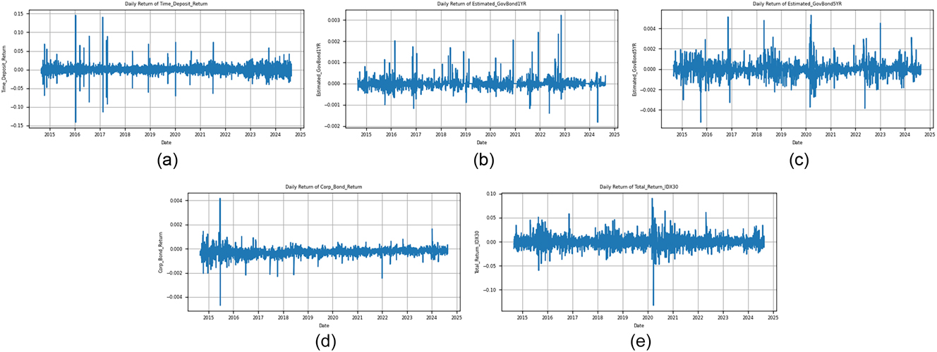
Cumulative return series from 2014 to 2024: (a) time deposits, (b) 1-year government bonds, (c) 5-year government bonds, (d) corporate bonds, and (e) IDX30 index.
We provide summary statistics for each asset in Table 1. Table 1 presents the mean return, volatility (standard deviation), skewness, kurtosis, and other relevant metrics for the five asset classes. Each return series has 2,449 observations. The mean returns differ across assets: time deposits have the lowest average return (reflecting their conservative nature), and equities have a higher mean return but also the highest volatility. Government bonds (1-year and 5-year) and corporate bonds fall in between, with moderate returns and low volatility. The distributional metrics indicate that all asset returns are roughly centered around zero on a daily basis, but their dispersion varies significantly. Equities exhibit negative skewness and high kurtosis (fat tails), hinting at occasional extreme losses, whereas time deposit returns are almost symmetric and light-tailed (very few extreme deviations).
Summary statistics of daily returns (2014–2024) for five Indonesian financial instruments: time deposits, government bonds (1-year and 5-year), corporate bonds, and IDX30 index.
| Deposit return | GovBond1YR | GovBond5YR | Corp bond return | IDX30 | |
|---|---|---|---|---|---|
| Count | 2,449.00 | 2,449.00 | 2,449.00 | 2,449.00 | 2,449.00 |
| Mean | −0.000144 | 0.016062 | 0.020732 | 0.000238 | 0.000242 |
| Std | 0.012782 | 0.084937 | 0.251563 | 0.000346 | 0.012549 |
| min | −0.127194 | −1.156559 | −1.911531 | −0.004152 | −0.082657 |
| 25 % | −0.005633 | −0.002398 | −0.076640 | 0.000068 | −0.006087 |
| 50 % | −0.000123 | 0.018496 | 0.028911 | 0.000208 | 0.000315 |
| 75 % | 0.005182 | 0.044906 | 0.125870 | 0.000383 | 0.006215 |
| Max | 0.164652 | 0.684402 | 1.927401 | 0.004712 | 0.152989 |
The mean returns show varying patterns across the indicators. GovBond1YR and GovBond5YR exhibit the highest mean returns (0.016062 and 0.020732, respectively), followed by IDX30 and Corporate Bond Return with slightly positive means (0.000242 and 0.000238). Notably, the calculated mean return for time deposits is slightly negative (−0.000144), which likely reflects minor measurement or timing effects, since in practice time deposits yield small positive interest. The standard deviations reveal that GovBond5YR has the highest volatility (0.251563), followed by GovBond1YR (0.084937), while Deposit Return and IDX30 have moderate volatility (0.012782 and 0.012549, respectively). Corporate Bond Return shows the lowest volatility (0.000346). The range between the minimum and maximum values further highlights the variability of each indicator, with GovBond5YR having the broadest range, followed by GovBond1YR.
The median values provide additional insights into the central tendency of each indicator. GovBond1YR and GovBond5YR have positive medians (0.018496 and 0.028911, respectively), while IDX30 and Corporate Bond Return also show positive medians (0.000315 and 0.000208). In contrast, Deposit Return has a slightly negative median (−0.000123). The 25th and 75th percentiles offer a glimpse into the distribution of each indicator. GovBond5YR displays the widest interquartile range, followed by GovBond1YR, indicating higher variability in these government bond returns. IDX30 and Deposit Return have similar interquartile ranges, while Corporate Bond Return exhibits the narrowest range.
These summary statistics suggest that government bond indicators (GovBond1YR and GovBond5YR) exhibit higher returns but also higher volatility, especially for the 5-year bonds. The IDX30, representing the stock market, shows moderate volatility with slightly positive returns. Corporate Bond Return displays low volatility with small, consistently positive returns. On the other hand, Deposit Return shows negative mean and median returns, which may indicate a challenging period for time deposits during the observed timeframe.
Table 2 presents the covariance matrix for the five financial instruments: Deposit Return, GovBond1YR, GovBond5YR, Corporate Bond Return, and IDX30. This matrix provides valuable insights into the relationships and risk characteristics of these assets. The diagonal elements represent the variances, with Deposit Return and IDX30 displaying the highest values (1.6 × 10⁻⁴), indicating greater volatility. The off-diagonal elements represent covariances, highlighting important relationships between assets. Notably, Deposit Return shows negative covariances with all other assets, suggesting its potential role as a hedge within the portfolio. Positive covariances are observed between 1-year bonds, 5-year bonds, and equities (IDX30), indicating these asset returns often move in the same direction (though the magnitude of covariance is low). In contrast, Corporate Bond Return shows weak covariances with most other assets, implying that it may offer diversification benefits in a portfolio.
Covariance matrix of daily returns for the five selected financial instruments.
| Deposit return | GovBond1YR | GovBond5YR | Corp bond return | IDX30 | |
|---|---|---|---|---|---|
| Deposit return | 1.6 × 10⁻⁴ | −1.1 × 10⁻⁷ | −2.8 × 10⁻⁷ | −6.2 × 10⁻⁸ | −5.5 × 10⁻⁶ |
| GovBond1YR | −1.1 × 10⁻⁷ | 5.4 × 10⁻⁸ | 5.6 × 10⁻⁸ | −2.3 × 10⁻¹⁰ | 3.6 × 10⁻⁷ |
| GovBond5YR | −2.8 × 10⁻⁷ | 5.6 × 10⁻⁸ | 4.8 × 10⁻⁷ | 1.5 × 10⁻⁹ | 3.0 × 10⁻⁶ |
| Corp bond return | −6.2 × 10⁻⁸ | −2.3 × 10⁻¹⁰ | 1.5 × 10⁻⁹ | 1.2 × 10⁻⁷ | −9.2 × 10⁻⁹ |
| IDX30 | −5.5 × 10⁻⁶ | 3.6 × 10⁻⁷ | 3.0 × 10⁻⁶ | −9.2 × 10⁻⁹ | 1.6 × 10⁻⁴ |
We further illustrate the distribution of daily returns in Figure 2. Subplots (a) to (d) show that returns are tightly concentrated around zero, indicating minimal daily fluctuations for time deposits and bonds. Specifically, time deposit returns cluster near 0 %, reflecting their inherent stability and low variability. Returns on one-year government bonds exhibit a similarly narrow distribution, consistent with the low volatility of short-term sovereign debt. Five-year government bonds display slightly wider dispersion, yet remain relatively stable, suggesting modest sensitivity to interest rate changes. Corporate bond returns are also centered around zero but with greater spread, indicating higher credit risk compared to government bonds. In contrast, IDX30 equity returns in subplot (e) exhibit a wider distribution with heavier tails, suggesting higher volatility and more frequent extreme movements, as is typical in equity markets. Overall, Figure 2 confirms that equity instruments carry the highest day-to-day risk, while fixed-income assets – particularly time deposits and government bonds – remain the most stable components of the portfolio.
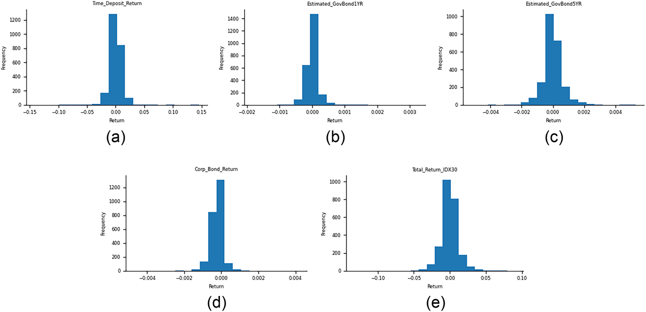
Distribution of daily returns: (a) time deposits, (b) 1-year government bonds, (c) 5-year government bonds, (d) corporate bonds, and (e) IDX30 equities – highlighting relative volatility and return concentration for each asset class.
Building on these asset characteristics, we conduct Conditional Value-at-Risk (CVaR) optimization to construct optimal portfolios under two scenarios: (i) without regulatory constraints, and (ii) with the constraints imposed by OJK Regulation No. 5 of 2023. In both settings, the objective is to maximize expected return for a given level of risk, where risk is measured using CVaR at a 99 % confidence level. The optimization is formulated as a linear programming problem, in which either the CVaR is minimized subject to a target return, or the return is maximized subject to a CVaR constraint – both approaches yield comparable outcomes. Regulatory constraints from the OJK regulation are incorporated as linear constraints on asset weights. For example, fixed-income assets are required to comprise between 65 % and 85 % of the portfolio, and equity investments are capped according to specified thresholds. In addition, short-selling is prohibited, and the sum of all portfolio weights must equal 100 %.
The optimal portfolio weights for each asset class are presented in Table 3. The results reveal a clear contrast between the unconstrained and constrained optimization scenarios. In the absence of regulatory limits, the optimizer produces a relatively balanced allocation across all five asset classes, with each receiving approximately 19–20 % of the total portfolio. Specifically, the weights are approximately 19.4 % in time deposits, 20.4 % in one-year government bonds, 20.4 % in five-year government bonds, 20.4 % in corporate bonds, and 19.4 % in equities (IDX30). This near-equal distribution suggests that, given the return-risk characteristics of the available assets, broad diversification is effective in minimizing tail risk – a well-known advantage of portfolio diversification. The optimizer appears to leverage the low correlations among asset classes and the relatively moderate returns of bonds to construct a stable portfolio. Notably, the unconstrained solution exhibits a slight preference for fixed-income instruments over equities, with approximately 80 % of the portfolio allocated to fixed-income assets (deposits and bonds) and the remaining 20 % to equities.
Optimal portfolio weights with and without constraints imposed by OJK Regulation No. 5 of 2023.
| Asset | Without constraint | With constraints |
|---|---|---|
| Deposit return | 0.1938 | 0.1551 |
| GovBond1YR | 0.2040 | 0.1312 |
| GovBond5YR | 0.2039 | 0.1311 |
| Corp bond return | 0.2041 | 0.3147 |
| IDX30 | 0.1939 | 0.2676 |
When the regulatory constraints of OJK Regulation No. 5 of 2023 are imposed, the optimal allocation shifts accordingly. The fixed-income portion of the portfolio now constitutes 73.21 %, which falls within the OJK-mandated range of 65–85 %, reflecting the conservative investment approach typically required of insurance portfolios (Chen and Hieber 2016). However, the internal composition of fixed-income assets becomes more uneven: 15.5 % in time deposits, 13.1 % in one-year government bonds, 13.1 % in five-year government bonds, and 31.5 % in corporate bonds. The remaining 26.8 % is allocated to equities, which remains within typical equity exposure limits (e.g., a 30 % cap).
Compared to the unconstrained case, the constrained portfolio exhibits a notable overweight in corporate bonds and equities. This shift arises partly because the regulation imposes upper limits on the allocation to safer instruments such as deposits and government bonds, and also encourages a broader mix of assets. In our model, we implemented OJK’s restriction that no more than 20 % of the portfolio may be allocated to any single instrument or asset class. While the unconstrained optimizer assigned approximately 19 % to time deposits – well within that cap – additional rules such as minimum requirements for corporate bond holdings and limits on government securities necessitated further rebalancing. To satisfy these constraints, the optimizer increases the allocation to corporate bonds, which offer relatively higher returns within the fixed-income universe, until the total fixed-income allocation reaches the required minimum. The residual allocation is then directed toward equities, up to the allowed maximum. The result is a more barbell-like structure: reduced exposure to ultra-low-yield instruments such as time deposits, increased investment in corporate bonds (which carry slightly higher risk but offer better returns), and a higher allocation to equities than in the unconstrained scenario.
The contrast between the unconstrained and constrained portfolios underscores the influence of regulatory constraints on optimal asset allocation. While the unconstrained solution favored an evenly diversified portfolio across all asset classes, the presence of regulatory limits in the constrained case led to a more skewed allocation. In particular, the requirement to maintain a fixed-income proportion within a specified range, combined with sub-limits on individual asset classes such as government bonds and time deposits, compelled the optimizer to allocate a larger share to corporate bonds. This adjustment was necessary to satisfy the fixed-income requirement while adhering to the upper bounds imposed on other safer instruments.
The optimization results demonstrate strict adherence to all specified constraints. No single asset exceeds the 35 % maximum allocation limit, and all assets maintain at least a 10 % allocation, satisfying both upper and lower bound constraints. The sum of all weights equals 1 (allowing for minor rounding errors), and no negative weights are present, meeting the non-negativity constraint that prohibits short-selling.
This carefully balanced allocation strategy prioritizes stability through a strong fixed-income base while allowing for growth potential through a significant equity component. The distribution across different fixed-income instruments (time deposits, government bonds of varying maturities, and corporate bonds) suggests a nuanced approach to managing interest rate risk and credit risk within the portfolio (Subramanian and Wang 2021).
We evaluate the performance of the two optimal portfolios on several metrics, including expected return, volatility, Value-at-Risk (VaR), CVaR, and Sharpe ratio. Table 4 compares the VaR and CVaR of the unconstrained versus constrained portfolios at different confidence levels. For each portfolio, the one-day VaR at 90 %, 95 %, and 99 % confidence levels is reported, along with the corresponding CVaR (average loss beyond VaR). For example, at 95 % confidence, the unconstrained portfolio has VaR
Comparison of portfolio risk metrics (VaR and CVaR) at multiple confidence levels between unconstrained and OJK-constrained portfolios.
| β | Unconstrained | Constrained | ||
|---|---|---|---|---|
| VaR | CVaR | VaR | CVaR | |
| 90 % | −0.0035 | −0.0058 | −0.0041 | −0.0066 |
| 95 % | −0.0049 | −0.0075 | −0.0058 | −0.0084 |
| 99 % | −0.0081 | −0.0128 | −0.0094 | −0.0132 |
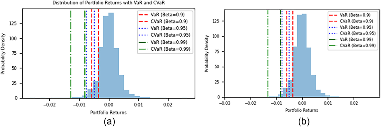
Distribution of portfolio returns with value at risk (VaR) and conditional value at risk (CVaR): (a) unconstrained portfolio, (b) OJK-constrained portfolio.
Figure 3 illustrates the distribution of portfolio returns, highlighting the Value at Risk (VaR) and Conditional Value at Risk (CVaR) at different confidence levels for the unconstrained portfolio on the left and the constrained one on the right. In subplot (a), the loss distribution of the unconstrained portfolio is narrower, indicating fewer extreme negative returns. The indicated VaR and CVaR levels (markers on the distribution) show that at a 99 % confidence level the portfolio’s worst-case daily loss is about 0.8 %, with an average loss of
Apart from tail risk, we also compare the expected returns and Sharpe ratios of the two portfolios. Both portfolios were optimized with a focus on risk, so their expected daily returns are relatively modest. Annualized, the constrained portfolio’s expected return is slightly higher (owing to its higher allocation in equities and corporate bonds, which carry risk premiums), whereas the unconstrained portfolio, being more conservative, has a slightly lower expected return. However, when adjusted for risk, both portfolios fare poorly by conventional metrics. The Sharpe ratio (mean excess return divided by standard deviation) comes out negative for both portfolios when using a zero or very low risk-free rate baseline. In our calculation, we treated the time deposit rate as a proxy for a risk-free rate (which is around 0.0–0.1 % per day in our dataset, effectively close to zero on a daily basis). The constrained portfolio’s Sharpe ratio is about −2.58, and the unconstrained portfolio’s Sharpe ratio is −2.89 (these are based on daily returns, which annualize to roughly −0.16 and −0.18 respectively when using standard 252 trading days). A negative Sharpe ratio means the portfolio’s return is lower than the risk-free rate, indicating that taking on risk actually detracted value relative to holding risk-free assets. In practical terms, a negative Sharpe ratio implies an investor would have been better off taking no risk (or just holding cash) than holding the portfolio. The more negative the Sharpe, the worse the risk-adjusted performance. In our results, both portfolios underperformed a zero-return benchmark, likely because the sample period included turbulent market episodes (e.g., 2015 downturn, 2020 crash) that dragged down average returns. The constrained portfolio has a less negative Sharpe than the unconstrained portfolio (−2.58 vs −2.89), which might seem surprising since the unconstrained portfolio was lower-risk. This occurs because the unconstrained portfolio’s expected return was also quite low (due to heavy allocation to very low-yield assets), so its excess return over “safe” rate was even more negative. Meanwhile, the constrained portfolio, by taking slightly more risk, earned a bit more return (though still not enough to be positive after risk-free), hence a slightly better Sharpe. When interpreting such negative Sharpe ratios, it’s important to note that comparisons become tricky – neither portfolio is attractive in absolute terms. One cannot meaningfully say a portfolio with Sharpe −2.5 is “good”; rather, it’s less bad than −2.9. In practice, a rational insurer would not aim for negative-Sharpe outcomes; these results underscore the challenge of the low-yield environment of the past decade. They also highlight that regulatory compliance can come at the cost of some return, though here it improved return at the expense of slightly higher risk, yielding a marginally better (less negative) Sharpe.
However, interpreting these results requires careful consideration of the broader context of insurance portfolio management. While the unconstrained portfolio appears to have a lower risk profile from a purely mathematical perspective, the constrained portfolio is designed to meet specific regulatory and strategic requirements crucial for insurance companies (Gaganis, Hasan, and Pasiouras 2020). The constraints often enforce diversification and adherence to regulatory limits, which, although potentially increasing short-term risk measures, can lead to more robust long-term performance and better protection against unforeseen market events (Xu et al. 2016).
The difference in risk measures between the two portfolios is relatively small, with the gap widening at higher confidence levels. This suggests that constraints have a more significant impact on extreme tail events, an important consideration for insurers focused on long-term stability and solvency (Huang et al. 2008). The slightly higher risk measures of the constrained portfolio may be a necessary trade-off for ensuring regulatory compliance and maintaining a balanced risk-return profile that aligns with the insurer’s long-term objectives (Forsyth 2020). The constrained portfolio, despite exhibiting slightly higher theoretical risk metrics, offers critical strategic advantages. These contains encourage diversification and prudent risk-taking, thus aligning closely with regulatory goals of maintaining financial health and ensuring long-term solvency in the Indonesian insurance market.
It’s important to note that lower risk measures do not necessarily indicate a superior portfolio strategy in the context of insurance asset management. The constrained portfolio, despite showing slightly higher risk, represents a more realistic and implementable approach in a regulated insurance environment (Zhang and Cao 2023). It likely offers a more balanced solution that considers not only risk minimization but also regulatory compliance, liquidity needs, and the ability to meet policyholder obligations (Peng and Li 2023).
Moreover, the comparison between constrained and unconstrained results provides valuable insights for risk managers and regulators. It highlights the potential impact of regulatory constraints on portfolio efficiency and may inform discussions on optimizing regulatory frameworks to achieve a better balance between risk control and investment performance (Subramanian and Wang 2021).
The comparison of portfolio optimization results with and without constraints reveals interesting differences in both portfolio composition and performance metrics. The constrained portfolio shows a more diverse asset allocation, with weights ranging from 13.11 % to 31.47 %, indicating a preference for certain assets over others. In contrast, the unconstrained portfolio allocates roughly 20 % to each asset, resembling a naive equal-weight strategy.
Finally, we illustrate the efficient frontiers with and without regulatory constraints in Figure 4. Each curve shows the minimum CVaR achievable for a range of target returns (or equivalently the maximum return for a given CVaR level), based on our five asset classes. The unconstrained frontier lies above and to the left of the constrained frontier. This indicates that without the OJK rules, an insurer could attain slightly higher returns for the same level of risk, or conversely, lower risk for the same return, compared to the regulated scenario. For example, to achieve an expected return of, say, 0.05 % per day, the unconstrained portfolio might attain a CVaR of 1.0 %, whereas the constrained one might have a CVaR of 1.2 %. The gap between the frontiers represents the opportunity cost of regulation – the loss of efficiency due to not being able to fully optimize. However, the difference is not extremely large, suggesting that OJK’s limits, while binding, do not completely derail efficient investing. In fact, the constrained frontier remains fairly close to the unconstrained one in our analysis, implying that the OJK rules still allow for near-optimal diversification (since the unconstrained optimum itself was well-diversified and within many of the OJK bounds naturally). The regulated frontier’s shape also reflects how the required fixed-income weighting provides downside protection (keeping CVaR from ballooning) at the expense of capping upside when higher returns would require more equity exposure.
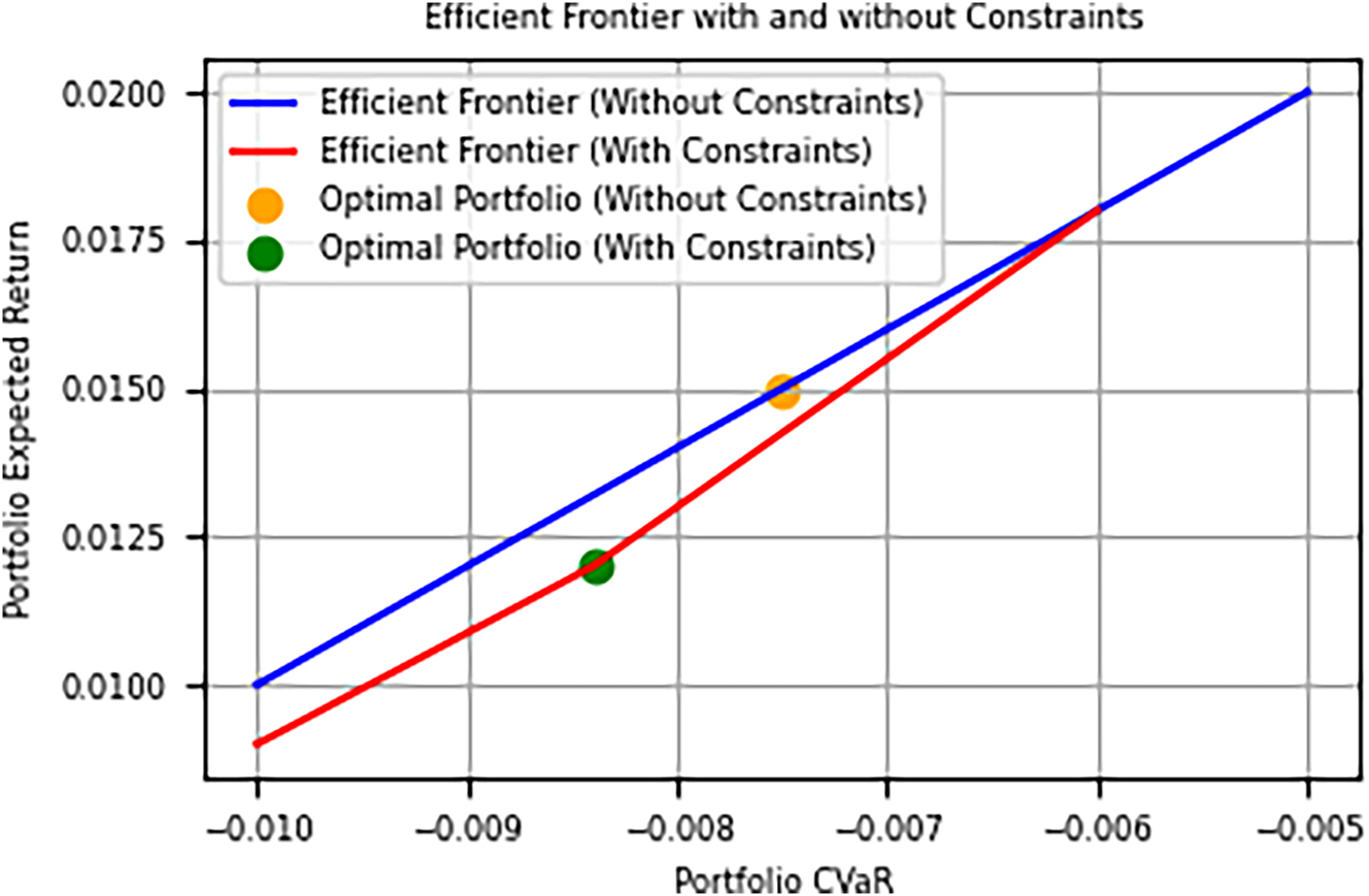
Efficient frontier comparison of optimized portfolios with and without OJK regulatory constraints.
4 Conclusions
This study has quantitatively assessed the impact of OJK Regulation No. 5 of 2023 on insurance portfolio construction using a CVaR-based optimization framework. We compared unconstrained and constrained portfolios, revealing that regulatory limits shape asset allocation by restricting excessive exposure to the safest instruments and enforcing diversification. The constrained portfolio exhibits a marginally higher CVaR and VaR across confidence levels, reflecting the cost of prudential safeguards in terms of tail-risk efficiency. Nevertheless, the allocation remains broadly consistent with risk-management goals, and the regulation does not drastically impair portfolio performance. The constrained portfolio still lies close to the efficient frontier and maintains a conservative structure suitable for insurers. However, both optimized portfolios showed negative Sharpe ratios over the observed period, underscoring the challenge of achieving positive risk-adjusted returns in a low-yield environment.
These findings have several implications. For insurers, the results demonstrate that CVaR-based optimization remains a valuable tool for navigating regulatory limits while pursuing efficiency. For regulators, the study highlights the importance of calibrating constraints to balance solvency with return potential – overly rigid rules may hinder performance without materially improving stability. The design of OJK’s framework, which aligns with international practices such as Solvency II, NAIC, and MAS guidelines, appears well-tuned to Indonesia’s current market structure.
Future research could extend this work by incorporating dynamic rebalancing, stress-testing under extreme scenarios, liability-driven investing, or evaluating the regulatory impact under different market conditions. Additional exploration of alternative asset classes permitted under regulation, such as real estate and infrastructure, may also help insurers enhance performance without compromising compliance.
Funding source: Universitas Gadjah Mada
Award Identifier / Grant number: Capstone Project Research Grant 2024
Acknowledgements
We would like to express our sincere gratitude to Mr. Doddy Vierzehn Putra and Mr. Henry Viriya Surya from PT Asuransi Tugu Pratama for their invaluable insights and support throughout this research. Their expertise and guidance have been instrumental in shaping the direction and outcomes of this study.
-
Research funding: This research was funded by Universitas Gadjah Mada under the Capstone Project Research Grant 2024, Number 356/UN1/JM/2024.
References
Acerbi, C., and P. Simonetti. 2002. “Portfolio Optimization with Spectral Measures of Risk.” arXiv preprint cond-mat/0203607. https://doi.org/10.48550/arXiv.cond-mat/0203607.Suche in Google Scholar
Armantier, O., J. Foncel, and N. Treich. 2023. “Insurance and Portfolio Decisions: Two Sides of the Same Coin?” Journal of Financial Economics 148 (3): 201–19.10.1016/j.jfineco.2023.03.003Suche in Google Scholar
Chen, An, and Peter Hieber. 2016. “Optimal Asset Allocation in Life Insurance: The Impact of Regulation.” ASTIN Bulletin 46 (3): 605–26. https://doi.org/10.1017/asb.2016.12.Suche in Google Scholar
Cheng, C., and J. Li. 2018. “Early Default Risk and Surrender Risk: Impacts on Participating Life Insurance Policies.” Insurance: Mathematics and Economics 78: 30–43. https://doi.org/10.1016/j.insmatheco.2017.11.001.Suche in Google Scholar
European Commission. 2009. Directive 2009/138/EC of the European Parliament and of the Council of 25 November 2009 on the Taking-Up and Pursuit of the Business of Insurance and Reinsurance (Solvency II). https://eur-lex.europa.eu/legal-content/EN/TXT/?uri=CELEX:32009L0138 (accessed May 5, 2025).Suche in Google Scholar
Forsyth, P. A. 2020. “Optimal Dynamic Asset Allocation for DC Plan Accumulation/decumulation: Ambition-CVaR.” Insurance: Mathematics and Economics 93: 230–45. https://doi.org/10.1016/j.insmatheco.2020.05.005.Suche in Google Scholar
Gaganis, C., I. Hasan, and F. Pasiouras. 2020. “Cross-country Evidence on the Relationship between Regulations and the Development of the Life Insurance Sector.” Economic Modelling 89: 256–72. https://doi.org/10.1016/j.econmod.2019.10.024.Suche in Google Scholar
Huang, D., S.-S. Zhu, F. J. Fabozzi, and M. Fukushima. 2008. “Portfolio Selection with Uncertain Exit Time: A Robust CVaR Approach.” Journal of Economic Dynamics and Control 32 (2): 594–623. https://doi.org/10.1016/j.jedc.2007.03.003.Suche in Google Scholar
Irhamni, F. 2024. “Constructing Portfolio Optimization: Analysis in Indonesia Non-cyclical Industry (Markowitz Approach and Skewness and Kurtosis).” Revista De Gestão Social E Ambiental 18 (5): e05645. https://doi.org/10.24857/rgsa.v18n5-099.Suche in Google Scholar
Markowitz, H. 1952. “Portfolio Selection.” The Journal of Finance 7 (1): 77–91. https://doi.org/10.1111/j.1540-6261.1952.tb01525.x.Suche in Google Scholar
McShane, M. K., L. A. Cox, and R. J. Butler. 2010. “Regulatory Competition and Forbearance: Evidence from the Life Insurance Industry.” Journal of Banking & Finance 34 (3): 522–32. https://doi.org/10.1016/j.jbankfin.2009.08.016.Suche in Google Scholar
Melina, Sukono, H. Napitupulu, and N. Mohamed. 2023. “A Conceptual Model of Investment-Risk Prediction in the Stock Market Using Extreme Value Theory with Machine Learning: A Semisystematic Literature Review.” Risks 11 (3): 60. https://doi.org/10.3390/risks11030060.Suche in Google Scholar
Monetary Authority of Singapore. 2020. Guidelines on Risk Management Practices for Insurers. https://www.mas.gov.sg/regulation/guidelines (accessed May 5, 2025).Suche in Google Scholar
National Association of Insurance Commissioners. 2021. Investment Law Handbook. Kansas City: NAIC Publications.Suche in Google Scholar
Oktavianus Yusan, B., and S. Riyadi. 2024. “Portfolio Optimization: Application and Comparison of Markowitz Model and Single Index Model on LQ45 Stocks in Indonesia Stock Exchange.” International Journal of Management Science and Application 3 (1): 57–85. https://doi.org/10.58291/ijmsa.v3i1.210.Suche in Google Scholar
Otoritas Jasa Keuangan, (OJK). 2023. Regulation No.5/2023 on Financial Health Standards for Insurance Companies. https://www.ojk.go.id/ (accessed May 3, 2025).Suche in Google Scholar
Peng, X., and B. Li. 2023. “Optimal Investment, Consumption and Life Insurance Purchase with Learning about Return Predictability.” Insurance: Mathematics and Economics 113: 70–95. https://doi.org/10.1016/j.insmatheco.2023.07.005.Suche in Google Scholar
Rockafellar, R. T., and S. Uryasev. 2000. “Optimization of Conditional Value-At-Risk.” Journal of Risk 2 (3): 21–41. https://doi.org/10.21314/jor.2000.038.Suche in Google Scholar
Semeru, I. M. G. A., and Y. A. Nainggolan. 2023. “Investment Portfolio Optimization in Indonesia (Study on: LQ-45 Stock Index, Government Bond, United States Dollar, Gold and Bitcoin).” International Journal of Current Science Research and Review 6 (7): 4922–34. https://doi.org/10.47191/ijcsrr/v6-i7-108.Suche in Google Scholar
Subramanian, A., and J. Wang. 2021. “Capital, Aggregate Risk, Insurance Prices and Regulation.” Insurance: Mathematics and Economics 100: 156–92. https://doi.org/10.1016/j.insmatheco.2021.05.003.Suche in Google Scholar
Susyanto, N., and C. A. J. Klaassen. 2017. “Semiparametrically Efficient Estimation of Constrained Euclidean Parameters.” Electronic Journal of Statistics 11 (2): 3120–40. https://doi.org/10.1214/17-ejs1308.Suche in Google Scholar
Uryasev, S. 2000. “Conditional Value-At-Risk: Optimization Algorithms and Applications.” In Proceedings of the IEEE/IAFE/INFORMS 2000 Conference on Computational Intelligence for Financial Engineering (CIFEr) (Cat. No.00TH8520), 49–57.10.1109/CIFER.2000.844598Suche in Google Scholar
Xu, Q., Y. Zhou, C. Jiang, K. Yu, and X. Niu. 2016. “A Large CVaR-Based Portfolio Selection Model with Weight Constraints.” Economic Modelling 59: 436–47. https://doi.org/10.1016/j.econmod.2016.08.014.Suche in Google Scholar
Yu, J.-R., W. P. Chiou, C.-H. Hung, W.-K. Dong, and Y.-H. Chang. 2022. “Dynamic Rebalancing Portfolio Models with Analyses of Investor Sentiment.” International Review of Economics & Finance 77: 1–13. https://doi.org/10.1016/j.iref.2021.09.003.Suche in Google Scholar
Zhang, T., and J. Cao. 2023. “Impact of Regulatory Policy Adjustments on Insurance Company Costs and Cost Efficiency.” Finance Research Letter 58 (Part D): 104611, https://doi.org/10.1016/j.frl.2023.104611.Suche in Google Scholar
© 2025 the author(s), published by De Gruyter, Berlin/Boston
This work is licensed under the Creative Commons Attribution 4.0 International License.
Artikel in diesem Heft
- Frontmatter
- Editorial
- Statistics, Politics and Policy, Volume 2/2025
- Special Issue: Emotional dynamics of politics and policymaking; Guest Editor: Georg Wenzelburger
- A State of the Art on Emotions in the Context of Public Policymaking
- Regular Articles
- Estimating Crowd: Electoral Adjustment and Spatial Effects of Turnout During Covid-19 Pandemic
- The Effect of Military Spending on Unemployment in South Africa: Evidence from Total, Gender, Race and Province Unemployment Data
- Investment Optimization in Insurance Portfolios: A Quantitative Analysis of Financial Services Authority of Indonesia Regulations