Bayesian Flexible Local Projections
-
Luca Brugnolini
 ,
Pernille Hansen
,
Pernille Hansen

Abstract
We develop a methodology to estimate impulse response functions via Bayesian techniques with the goal of providing a bridge between a linear vector autoregressive specification and a high-order polynomial local projection, namely flexible local projection. We label this methodology Bayesian Flexible Local Projection (BFLP). We assess the properties of BFLP in a Monte Carlo framework considering both linear and non-linear models as data generating processes. We also empirically illustrate how BFLP can be used with standard identification strategies. In particular, we show how to use external instruments to identify the effects of the monetary policy shock in the United States. Furthermore, exploiting the time-varying nature of the impulse response functions based on BFLP, we assess the zero lower bound irrelevance hypothesis and find no strong evidence that monetary policy was less effective in influencing output and inflation during the recent ZLB period.
Funding source: Danmarks Frie Forskningsfond
Award Identifier / Grant number: 3099-00089B
Appendix A: Posterior Density and Marginal Likelihood
This appendix derives the analytical expression of the posterior density of Bayesian Local Projections (BLP) with conjugate priors exploiting results from Appendix A of Giannone, Lenza, and Primiceri (2015), and of the marginal likelihood. The appendix concludes by presenting a way to compute the marginal likelihood in a numerically stable way which is then used for Markov chain Monte Carlo estimation of the BLP coefficients.
A.1 Derivation of the Posterior Density
Consider the vec representation in (6) where the superscript
The term E can be rewritten as
Let now:
then E can then be rewritten as
where
Inserting the definitions of w and W from Equation (21) in the OLS estimator yields
Furthermore, given that
and
it follows that, letting
Thus, the exponent E in Equation (19) further reduces to
Inserting E from equation in the joint density of
where
The marginal likelihood is then given as
A.2 Stable Marginal Likelihood
The marginal likelihood in Equation (30) is numerically unstable for large systems, and is therefore replaced by the equivalent expression
where
Appendix B: Markov-Chain Monte-Carlo Algorithm
The posterior of the hyperparameter
is proportional to the fit-complexity trade-off representation of Giannone, Lenza, and Primiceri (2015)
where
with mode of the distribution fixed at 0.4 and standard deviation following a logistic function
. The logistic function is increasing in the horizon that taps of at horizons larger than h = 36, implying an increasingly diffuse prior in the forecast horizon h, consistent with the notion that prior model misspecification is compounded at each horizon.
B.1 λ (h) under Estimation Uncertainty
Drawing from the posterior when
Algorithm B.1:
MCMC with Metropolis-Hastings updating of prior tightness.
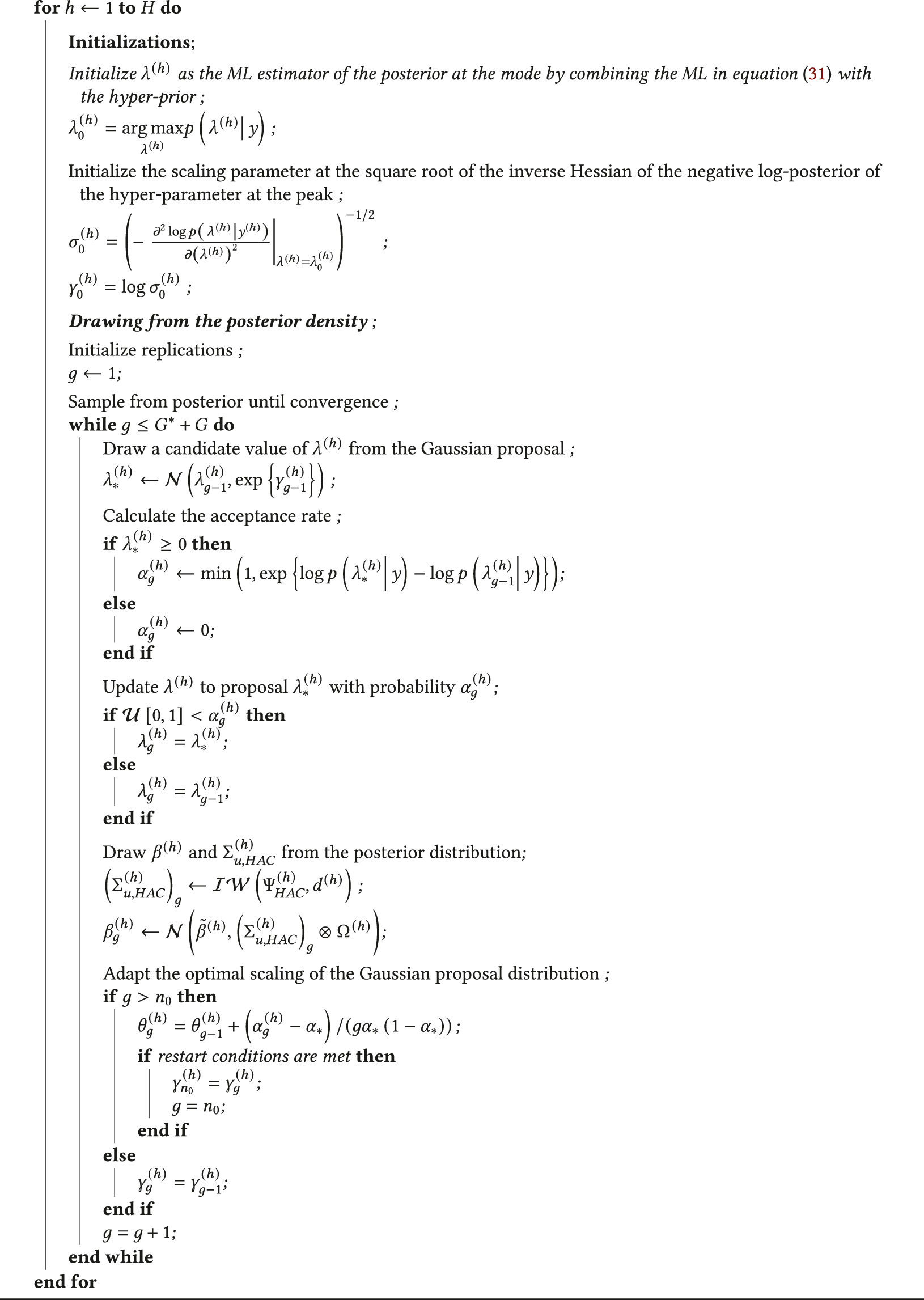
We follow Giannone, Lenza, and Primiceri (2015) and update the prior tightness parameter according to a Metropolis-Hastings algorithm, where at each iteration a candidate value is drawn from a Gaussian proposal with mean equal to the preceding value in the Markov chain,
The search is restarted at the previous estimate of γ* and jumps back to
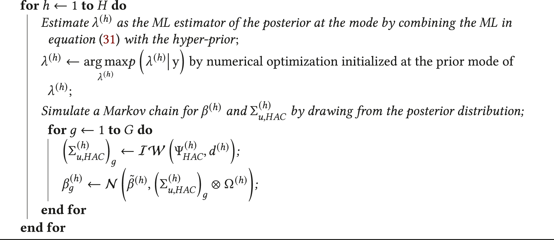
B.2 λ (h) Estimated via Maximum Posterior
When
Algorithm B.2:
MCMC Setup for BLP with Fixed Prior Tightness at the ML Estimator
References
Barnichon, R., and C. Brownlees. 2019. “Impulse Response Estimation by Smooth Local Projections.” Review of Economics and Statistics 101 (3): 522–30. https://doi.org/10.1162/rest_a_00778.Search in Google Scholar
Barnichon, R., and C. Matthes. 2018. “Functional Approximation of Impulse Responses.” Journal of Monetary Economics 99: 41–55. https://doi.org/10.1016/j.jmoneco.2018.04.013.Search in Google Scholar
Brugnolini, L. 2018. “About Local Projection Impulse Response Function Reliability.” CEIS (Tor Vergata) Research Paper Series Nr. 440 (6): 16.10.2139/ssrn.3229218Search in Google Scholar
Campbell, J. R., C. L. Evans, J. D. Fisher, and A. Justiniano. 2012. “Macroeconomic Effects of Federal Reserve Forward Guidance.” Brookings Papers on Economic Activity 2012 (1): 1–80. https://doi.org/10.1353/eca.2012.0004.Search in Google Scholar
Christiano, L., M. Eichenbaum, and C. Evans. 1999. “Monetary Policy Shocks: What Have We Learned and to what End?” In Handbook of Macroeconomics. 1st ed., Vol. 1, Part A Taylor, and M. Woodford, 65–148. North-Holland, Amsterdam, Holland: Elsevier. chapter 02.10.1016/S1574-0048(99)01005-8Search in Google Scholar
Christiano, L., M. Eichenbaum, and C. Evans. 2005. “Nominal Rigidities and the Dynamic Effects of a Shock to Monetary Policy.” Journal of Political Economy 113 (1): 1–45. https://doi.org/10.1086/426038.Search in Google Scholar
Coibion, O. 2012. “Are the Effects of Monetary Policy Shocks Big or Small?” American Economic Journal: Macroeconomics 4 (2): 1–32. https://doi.org/10.1257/mac.4.2.1.Search in Google Scholar
Cox, D. R. 1961. “Prediction by Exponentially Weighted Moving Averages and Related Methods.” Journal of the Royal Statistical Society. Series B (Methodological) 23 (2): 414–22. https://doi.org/10.1111/j.2517-6161.1961.tb00424.x.Search in Google Scholar
Debortoli, D., J. Galí, and L. Gambetti. 2020. “On the Empirical (Ir) Relevance of the Zero Lower Bound Constraint.” NBER Macroeconomics Annual 34 (1): 141–70. https://doi.org/10.1086/707177.Search in Google Scholar
Doan, T., R. Litterman, and C. Sims. 1984. “Forecasting and Conditional Projection Using Realistic Prior Distributions.” Econometric Reviews 3 (1): 1–100. https://doi.org/10.1080/07474938408800053.Search in Google Scholar
Ferreira, L. N., S. Miranda-Agrippino, and G. Ricco. 2023 In press. “Bayesian Local Projections.” The Review of Economics and Statistics 1–45, https://doi.org/10.1162/rest_a_01334.Search in Google Scholar
Garthwaite, P. H., Y. Fan, and S. A. Sisson. 2016. “Adaptive Optimal Scaling of Metropolis-Hastings Algorithms Using the Robbins-Monro Process.” Communications in Statistics – Theory and Methods 45 (17): 5098–111. https://doi.org/10.1080/03610926.2014.936562.Search in Google Scholar
Gertler, M., and P. Karadi. 2015. “Monetary Policy Surprises, Credit Costs, and Economic Activity.” American Economic Journal: Macroeconomics 7 (1): 44–76. https://doi.org/10.1257/mac.20130329.Search in Google Scholar
Geweke, J. 1992. “Evaluating the Accuracy of Sampling-Based Approaches to the Calculation of Posterior Moments.” In Bayesian Statistics, 169–94. Oxford: Oxford University Press.10.1093/oso/9780198522669.003.0010Search in Google Scholar
Giannone, D., M. Lenza, and G. E. Primiceri. 2015. “Prior Selection for Vector Autoregressions.” The Review of Economics and Statistics 97 (2): 436–51. https://doi.org/10.1162/rest_a_00483.Search in Google Scholar
Gürkaynak, R. S., B. Sack, and E. T. Swanson. 2005. “Do Actions Speak Louder Than Words? The Response of Asset Prices to Monetary Policy Actions and Statements.” International Journal of Central Banking 1 (1): 55–93.10.2139/ssrn.633281Search in Google Scholar
Herbst, E. P., and B. K. Johannsen. 2024. “Bias in Local Projection.” Journal of Econometrics 240 (1): 105655, https://doi.org/10.1016/j.jeconom.2024.105655.Search in Google Scholar
Ishwaran, H., and J. S. Rao. 2005. “Spike and Slab Variable Selection: Frequentist and Bayesian Strategies.” Annals of Statistics 33 (2): 730–73. https://doi.org/10.1214/009053604000001147.Search in Google Scholar
Jordá, O. 2005. “Estimation and Inference of Impulse Responses by Local Projections.” American Economic Review 95 (1): 161–82. https://doi.org/10.1257/0002828053828518.Search in Google Scholar
Jordà, Ò., and S. Kozicki. 2011. “Estimation and Inference by the Method of Projection Minimum Distance: An Application to the New Keynesian Hybrid Phillips Curve.” International Economic Review 52 (2): 461–87. https://doi.org/10.1111/j.1468-2354.2011.00635.x.Search in Google Scholar
Jordá, O., and K. Salyer. 2003. “The Response of Term Rates to Monetary Policy Uncertainty.” Review of Economic Dynamics 6 (4): 941–62. https://doi.org/10.1016/s1094-2025(03)00022-x.Search in Google Scholar
Jordà, O. 2009. “Simultaneous Confidence Regions for Impulse Responses.” Review of Economics and Statistics 91 (3): 629–47. https://doi.org/10.1162/rest.91.3.629.Search in Google Scholar
Justiniano, A., G. Primiceri, and A. Tambalotti. 2010. “Investment Shocks and Business Cycles.” Journal of Monetary Economics 57 (2): 132–45. https://doi.org/10.1016/j.jmoneco.2009.12.008.Search in Google Scholar
Kilian, L., and Y. J. Kim. 2011. “How Reliable Are Local Projection Estimators of Impulse Responses?” Review of Economics and Statistics 93 (4): 1460–6. https://doi.org/10.1162/rest_a_00143.Search in Google Scholar
Koop, G., M. Pesaran, and S. Potter. 1996. “Impulse Response Analysis in Nonlinear Multivariate Models.” Journal of Econometrics 74 (1): 119–47. https://doi.org/10.1016/0304-4076(95)01753-4.Search in Google Scholar
Lewis, R., and G. C. Reinsel. 1985. “Prediction of Multivariate Time Series by Autoregressive Model Fitting.” Journal of Multivariate Analysis 16 (3): 393–411. https://doi.org/10.1016/0047-259x(85)90027-2.Search in Google Scholar
Li, D., M. Plagborg-Møller, and C. K. Wolf. 2022. Local Projections vs. VARs: Lessons from Thousands of DGPs. NBER Working Paper 30207.10.3386/w30207Search in Google Scholar
Litterman, R. 1986. “Forecasting with Bayesian Vector Autoregressions – Five Years of Experience.” Journal of Business & Economic Statistics 4 (1): 25–38. https://doi.org/10.2307/1391384.Search in Google Scholar
McCallum, J. 1991. “Credit Rationing and the Monetary Transmission Mechanism.” The American Economic Review 81 (4): 946–51.Search in Google Scholar
Mertens, K., and M. O. Ravn. 2013. “The Dynamic Effects of Personal and Corporate Income Tax Changes in the United States.” American Economic Review 103 (4): 1212–47. https://doi.org/10.1257/aer.103.4.1212.Search in Google Scholar
Miranda-Agrippino, S., and G. Ricco. 2021. “The Transmission of Monetary Policy Shocks.” American Economic Journal: Macroeconomics 13 (3): 74–107. https://doi.org/10.1257/mac.20180124.Search in Google Scholar
Miranda-Agrippino, S., and G. Ricco. 2023. “Identification with External Instruments in Structural VARs.” Journal of Monetary Economics 135: 1–19. https://doi.org/10.1016/j.jmoneco.2023.01.006.Search in Google Scholar
Montiel Olea, J. L., and M. Plagborg-Møller. 2021. “Local Projection Inference is Simpler and More Robust Than You Think.” Econometrica 89 (4): 1789–823. https://doi.org/10.3982/ecta18756.Search in Google Scholar
Plagborg-Møller, M., and C. K. Wolf. 2021. “Local Projections and VARs Estimate the Same Impulse Responses.” Econometrica 89 (2): 955–80. https://doi.org/10.3982/ecta17813.Search in Google Scholar
Potter, S. 2000. “Nonlinear Impulse Response Functions.” Journal of Economic Dynamics and Control 24 (10): 1425–46. https://doi.org/10.1016/s0165-1889(99)00013-5.Search in Google Scholar
Priestley, M. B. 1988. Non-Linear and Non-Stationary Time Series Analysis. London: Academic Press.Search in Google Scholar
Ramey, V. A. 2016. “Macroeconomic Shocks and Their Propagation.” Handbook of Macroeconomics 2: 71–162. https://doi.org/10.1016/bs.hesmac.2016.03.003.Search in Google Scholar
Rao Kadiyala, K., and S. Karlsson. 1993. “Forecasting with Generalized Bayesian Vector Auto Regressions.” Journal of Forecasting 12 (3–4): 365–78. https://doi.org/10.1002/for.3980120314.Search in Google Scholar
Roberts, G. O., and J. S. Rosenthal. 2001. “Optimal Scaling for Various Metropolis-Hastings Algorithms.” Statistical Science 16 (4): 351–67. https://doi.org/10.1214/ss/1015346320.Search in Google Scholar
Sims, C. 1980. “Macroeconomics and Reality.” Econometrica 48 (1): 1–48. https://doi.org/10.2307/1912017.Search in Google Scholar
Sims, C., S. M. Goldfeld, and J. D. Sachs. 1982. “Policy Analysis with Econometric Models.” Brookings Papers on Economic Activity 13 (1): 107–64. https://doi.org/10.2307/2534318.Search in Google Scholar
Stock, J. H., and M. W. Watson. 2012. Disentangling the Channels of the 2007–2009 Recession. NBER Working Paper, 18094.10.3386/w18094Search in Google Scholar
Swanson, E. T., and J. C. Williams. 2014. “Measuring the Effect of the Zero Lower Bound on Medium-and Longer-Term Interest Rates.” American Economic Review 104 (10): 3154–85. https://doi.org/10.1257/aer.104.10.3154.Search in Google Scholar
Tenreyro, S., and G. Thwaites. 2016. “Pushing on a String: US Monetary Policy is Less Powerful in Recessions.” American Economic Journal: Macroeconomics 8 (4): 43–74. https://doi.org/10.1257/mac.20150016.Search in Google Scholar
Supplementary Material
This article contains supplementary material (https://doi.org/10.1515/snde-2023-0001).
© 2024 Walter de Gruyter GmbH, Berlin/Boston
Articles in the same Issue
- Frontmatter
- Editorial
- Editorial Introduction of the Special Issue of Studies in Nonlinear Dynamics and Econometrics in Honor of Herman van Dijk
- Review
- Challenges and Opportunities for Twenty First Century Bayesian Econometricians: A Personal View
- Research Articles
- Markov-Switching Models with Unknown Error Distributions: Identification and Inference Within the Bayesian Framework
- Dynamic Shrinkage Priors for Large Time-Varying Parameter Regressions Using Scalable Markov Chain Monte Carlo Methods
- Matrix autoregressive models: generalization and Bayesian estimation
- Sequential Monte Carlo with model tempering
- Modeling Corporate CDS Spreads Using Markov Switching Regressions
- Combining Large Numbers of Density Predictions with Bayesian Predictive Synthesis
- Bayesian inference for non-anonymous growth incidence curves using Bernstein polynomials: an application to academic wage dynamics
- Bayesian Reconciliation of Return Predictability
- A Dynamic Latent-Space Model for Asset Clustering
- Posterior Manifolds over Prior Parameter Regions: Beyond Pointwise Sensitivity Assessments for Posterior Statistics from MCMC Inference
- Bayesian Flexible Local Projections