
A solution for transverse thermal conductivity of composites with quadratic or hexagonal unidirectional fibres
-
Xueliang Xiao
 and
Andrew Long
and
Andrew Long

Abstract
A solution for the transverse thermal conductivity (Ke) of unidirectional fibre arrays, quadratic and hexagonal, is developed analytically. The solution integrates the thermal conductivity of fibre (Kf) and fluid (Km) based on electricity analogy without thermal contact resistance (Rc) at the fibre/fluid interface. The expression Ke is a function of Kf and Km, as well as of the fibre volume fraction (Vf). In this article, Ke values of four composites were predicted and verified by computational fluid dynamics (CFD) simulations. The results showed good agreement when the ratio of Kf/Km is close to 1. An increase in the ratio or Vf gives poorer agreement owing to the local temperature gradient at the fibre/fluid interface. CFD simulation also showed that Ke is decreasing as the Rc value increases.
Nomenclature
- dy
Width of an infinitesimal element
- f
Shape-related factor
- h
Height of hexagonal unit-cell, m
- Ke
Thermal conductivity of total materials, W/m·K
- Kf
Thermal conductivity of fibres, W/m·K
- Km
Thermal conductivity of matrix or fluid, W/m·K
- Kb
Thermal conductivity of thermal barrier, W/m·K

Heat flux, W/m2
- r
Length in fibre region, perpendicular to heat flow
- R
Fibre radius, m
- Rc
Thermal resistance at fibre/fluid interface, K/W
- Re
Absolute thermal resistance of total materials, K/W
- Rf
Absolute thermal resistance of fibres, K/W
- Rm
Absolute thermal resistance of matrix or fluid, K/W
- ΔT
Temperature drop, K
- Vf
Fibre volume fraction
- α
Fluid region with constant temperature gradient
- β
Fluid region with variable temperature gradient
1 Introduction
The transverse thermal conductivity of unidirectional fibre composites, in a quantitative manner, describes the ease of heat transfer in through-thickness under a temperature gradient. It is an important property for the application of composites in heat resistance areas, such as in a few industries like automotive, aircraft, and space clothing. Fibre spatial arrays and their effect on thermal conductivity have received large attention in the last decade. Therefore, an analytical solution for the effective thermal conductivity (Ke) is attractive for this kind of composite.
In the last decade, investigation has focused on the thermal conductivity of fibrous composites, using analytical approaches [1–3], numerical solutions [4, 5], and experiments [6–8]. For analytical modelling, two schemes were mostly mentioned [9–11] based on thermal conduction in parallel [Eq. (1)] and series [Eq. (2)]:
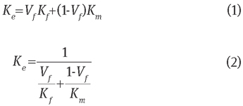
where Vf is the fibre volume fraction defined as the fibre volume divided by the composite volume, and Kf and Km are the thermal conductivity of the fibre and the matrix, respectively. These two equations are of limited usefulness and are only valid for the layers of dispersed phase aligned parallel or perpendicular to heat flow, giving coarse predictions for the Ke values of fibre-based composites.
Figure 1 shows three binary-phase geometries with the same Vf value. Provided with the same temperature drop, it is inevitable that they have different thermal resistances to the heat flow. On the basis of this issue, Carson and Sekhon [10] proposed a weighted harmonic mean of the series and parallel, where the weight parameter f (sometimes referred to as the “distribution factor”) has a value ranging between 0 and 1:
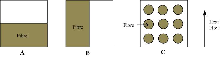
Binary-phase geometries of (A) series, (B) parallel and (C) unidirectional fibres distribution.
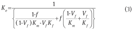
In principle, the thermal conductivity of any structure can be predicted with a suitable f, as the value should be somewhere between the series and parallel models. A number of attempts [12–14] have been made to use f as a shape-related factor, in the case of materials with distinct dispersed and continuous phase. However, the form of f in terms of materials distribution is still unknown. Nonetheless, the parallel model [Eq. (1)] is suitable for the Ke of longitudinal fibres, and the transverse Ke prediction was proposed [15, 16]:
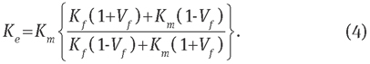
Eq. (4) is for the Ke of out-of-plane lamina, which is not accurate for the unidirectional fibre composite as the space between laminates is not the same as among fibres. On the basis of the Springer model [1], Tai [17] developed a general thermal conductivity model for heat transfer to elliptical cross-sectional fibres using the shear loading analogy, which can be converted into circular fibres:
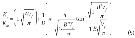
where 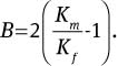 Eq. (5) is applicable when Kf is greater than Km. However, the author did not verify it by simulation or experiment, apart from discussion of Ke dependence on the fibre shape. Zinoviev and Smerdov [18] developed another Ke expression for the unidirectional fibre composite:
Eq. (6) is, in particular, for the Ke of composites containing identical fibres and matrix. However, the author did not validate it by experimental data either. Based on the electricity analogy, Rodriguez and Cabeza [19] obtained the thermal conductivity of a unit cell using finite element analysis, providing a reference to the present model.
Compared with the previous models, the aim of this article is to develop a more effective solution for the thermal conductivity of unidirectional fibre composites, in particular quadratic and hexagonal fibre arrays in composites. Considering the fibre distributions, a novel analytical model is developed on the basis of electricity analogy theory. The analytical solution is thereafter verified by computational fluid dynamics (CFD) simulation.
2 Theoretical analysis
2.1 Analytical solution
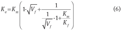
Two fibre arrays are common in unidirectional fibrous composites, quadratic and hexagonal, as shown in Figure 2. The dashed frames in Figure 2 represent the unit cell of fibre arrays. It is assumed that the fibres are impregnated in a fluid phase (air, water or resin). The thermal contact resistance at the fibre/fluid interface is assumed to be zero. In Figure 2A, the side length of unit cell and the fibre radius are supposed to be 2 and R (R≤1), respectively. A quarter of the unit cell is placed on x-y coordinates as shown in Figure 3.
Cross-section of idealized unidirectional fibre arrays: (A) quadratic and (B) hexagonal.
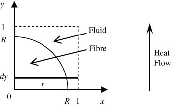
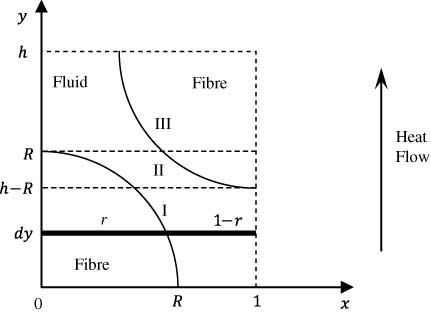
Heat flow in a quarter cross-section of quadratic fibre array.
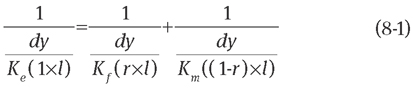
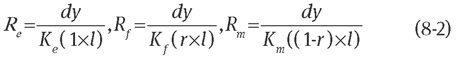
An infinitesimal element with a width dy parallel to the x-axis is shown in Figure 3. The element has a length r in the fibre and 1-r in the fluid. According to the electricity analogy [Eqs. (7-1) and (7-2)] and theory of thermal resistance [Eq. (7-3), Rb], there are [20]

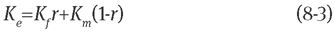
where A is the area of the element along the fibre axis and perpendicular to the heat flow. On the basis of the link of Rb and K in Eq. (7-3), Eqs. (7-1) and (7-2) can be used to obtain the parallel [Eq. (1)] and series [Eq. (2)] models, respectively. Herein, as shown in Figure 3, when the element is in the range of 0 and R along the y-axis, the Ke value of the element [Eq. (8-3)] is derived from Eqs. (7-1) and (7-3) as follows:
Thus,
where l is the length along the fibre axis. If the element goes from R to 1, Ke equals to Km. A combination of the element in both regions according to Eq. (7-2) gives Ke for the quarter of the unit cell:
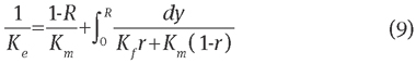
where  Setting y=R sinθ, the integration part of Eq. (9) becomes
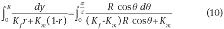
Eq. (10) has the following solution:
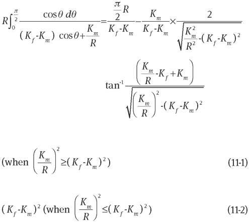
Substituting Eq. (11) into Eq. (9), Ke is then a function of Kf, Km and the fibre radius R. The fibre volume fraction is calculated as
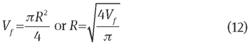
Therefore, Ke in Eq. (9) becomes a function of the fibre volume fraction if the fibre and fluid are known based on Eqs. (11) and (12):
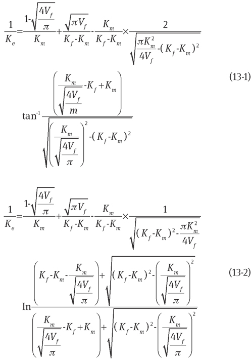
Eq. (13) is Ke for the quadratic fibre array. When to apply Eq. (13-1) or Eq. (13-2) depends on the amount of 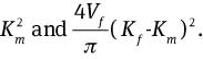
For the dashed rectangle in Figure 2B, it is placed in x-y coordinates as shown in Figure 4. Its width, height and fibre radius are set to be 1, h and R, respectively. Figure 4 shows heat flow through a higher Vf of the hexagonal fibre array (h<2R). An infinitesimal element is given with width dy, length r in fibre and 1-r in fluid as shown in region I of Figure 4. The element also passes regions II and III along the y-axis in the unit cell (Figure 4). The Re expressions for the three regions are given according to Eqs. (7) and (8):
Heat flow in a quarter cross-section of hexagonal fibre array.
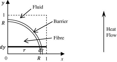
Heat flow in a quadratic unit cell with a thermal barrier on the fibre surface.
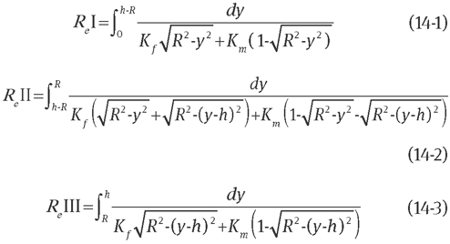
The three regions are connected in series [Eq. (7-2)] according to the electricity analogy. The Ke expression for the hexagonal unit cell based on Eq. (7-3) is
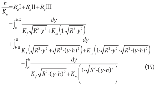
In Figure 4, the fibre volume fraction (Vf) is
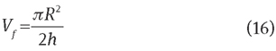
A combination of Eqs. (15) and (16) gives that Ke for the hexagonal fibre array is also a function of Kf, Km, R and Vf. An extension is given to the above equations [Eqs. (13) and (15)] when the fibre/fluid interface is covered by a thin material with a thermal conductivity Kb, as shown in Figure 5 which is the derivation of Figure 3. Owing to the limited thickness of the thermal barrier (dr), the element in the fluid has an approximate length of (1-r-dr). Then, Eq. (9) is modified as
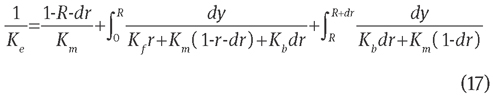
Eq. (17) is a simplified expression when dr<<R. Otherwise, more details about the derivation of the large thickness of thermal barrier can be found in Zou et al.’s [21] and Rocha and Cruz’s [22] works.
2.2 Verification
Numerical simulation was used to verify the current Ke solutions. Composite geometries were generated by TexGen [23] and exported as STEP files. The files were meshed by HyperMesh [24] with tetrahedron element shape and element size of 0.01 mm3 after a sensitivity study. The meshed geometries were imported into the CFD program [25] as BDF files. The top and bottom walls of the geometries were all set with a temperature drop of 50 K, and other boundaries were set as adiabatic or symmetric. The thermal contact resistance at interface was set as zero. During the simulations, the effect of thermal convection and radiation were ignored. In CFX-Post, the wall heat flux  can be calculated through the AreaAve function. The simulated Ke value of the meshed geometry was obtained [4]:
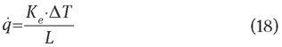
where ΔT/L is the temperature gradient for the geometry. In the CFD simulation, Table 1 lists the specifications of composite materials. The Vf values used are listed in Table 2, where the side length of the geometry was set as 1. Herein, experimental verification to the Ke solution is not included owing to the current development of a device for thermal conductivity measurement in our department.
Specifications of materials in CFD simulation.
| Materials | Air at 298K | Cotton | Glass fibre | Nylon6 | Concrete dense fibre |
|---|---|---|---|---|---|
| Density (kg/m3) | 1.185 | 1550 | 2550 | 1200 | 2100 |
| Specific heat capacity (J/(kg·K)) | 1004.4 | 1162 | 810 | 748.9 | 840 |
| Thermal conductivity (W/(m·K)) | 0.026 | 0.03 | 0.043 | 0.25 | 1.40 |
Fibre volume fractions (Vf) used in CFD simulation.
| Fibre radius (mm) | 0.250 | 0.500 | 0.750 | 0.833 | 0.875 | 0.917 | 0.958 | 0.983 |
|---|---|---|---|---|---|---|---|---|
| Vf | 0.049 | 0.196 | 0.442 | 0.545 | 0.601 | 0.660 | 0.721 | 0.759 |
3 Results and discussion
3.1 Comparison with previous models
The Ke values along Vf based on Eq. (13) were compared with predictions from reviewed models. In Figure 6, which shows the plots of the series, parallel, out-of-plane lamina, Tai model, Zinoviev model and the present model for Vf values from 0 to the maximum value 0.785 (quadratic), most curves lie between the upper and lower thermal conductivity limits (i.e., the parallel and series predictions). This also gives f values in Eq. (3) in terms of fibre distributions. However, Eq. (5) displays wrong predictions because of its lower Ke of the composite than that of materials inside.
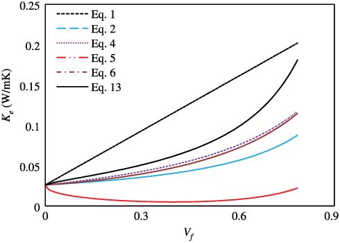
Plots of Eqs. (1), (2), (4), (5), (6), and (13) over the range of composition for a binary-phase material (nylon6 fibres in air at 298 K).
Figure 6 shows close predictions of Eqs. (4) and (6). Both curves increase slowly as Vf increases. Ke based on Eq. (13) shows a similar trend with both curves at low Vf values, while it increases significantly close to the prediction of Eq. (1) at high Vf values. This is true as Ke closes to the Km value at low Vf values but reaches the Kf value as Vf increases. However, its accuracy requires further verification by CFD simulation.
3.2 Ke of quadratic fibre array
Figure 7 compares Ke values predicted by Eq. (13) and reviewed models with simulated data. Four sets of binary-phase composites are verified, and the ratio values of Kf/Km are labelled in figures. Figure 7 shows that all the models can predict Ke accurately across the entire Vf values when the ratio is close to 1. This indicates that the current model can predict the thermal conductivity accurately for the textile fibres within quadratic array in air, such as cotton, wool and flax fibres. However, if the ratio is increased, most models only give good predictions for Ke at low Vf values, as shown in Figure 7C and D. A large difference appears between the simulated data and predictions at high Vf values. However, Ke based on Eq. (13) shows a dramatic increase with the increase of Vf. This is close to CFD simulations. However, the steep increase at high Vf values cannot be predicted by the reviewed models, indicating the advantage of the current model. Table 3 compares the errors between CFD-simulated and analytical predicted values, showing the relative accuracy of Eq. (13). However, the inaccurate predictions by Eq. (13) compared against CFD data indicate that a factor should be considered in the model development, which might be the local temperature gradient at the fibre/fluid interface.
Difference between CFD simulations and analytical predictions [Eqs. (2), (4), and (13)].
![Table 3 Difference between CFD simulations and analytical predictions [Eqs. (2), (4), and (13)].](/document/doi/10.1515/secm-2012-0146/asset/graphic/secm-2012-0146_tbl1.jpg)
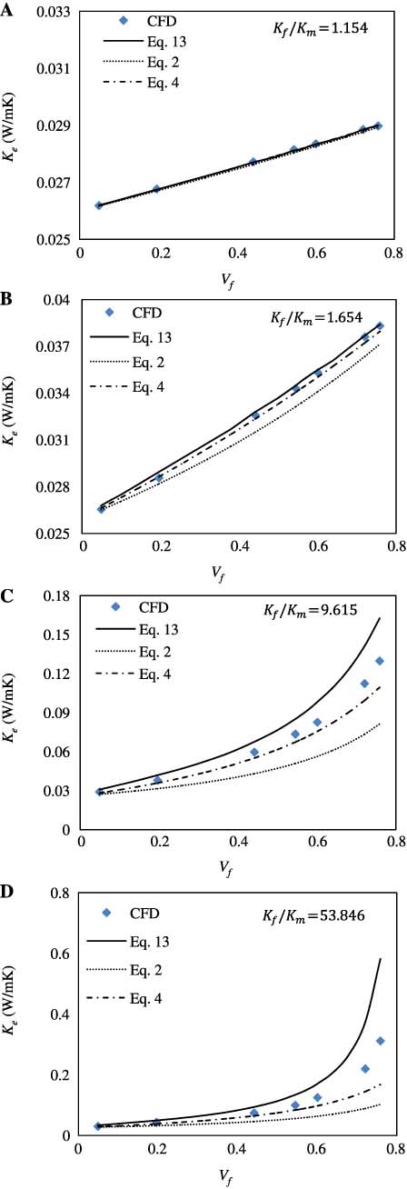
Comparison of predictions by the present model and reviewed models with CFD simulations along Vf values: (A) cotton/air, (B) glass fibre/air, (C) nylon6/air and (D) concrete dense fibre/air.
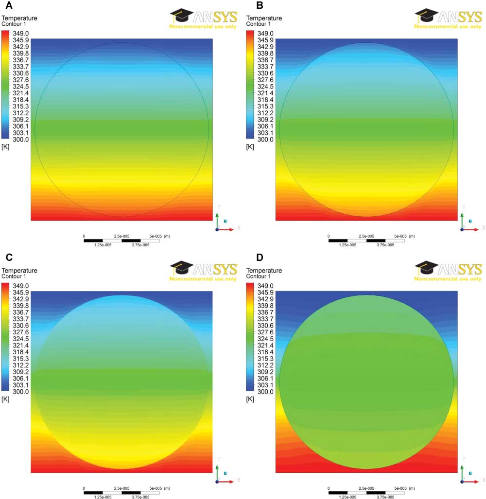
Figure 8 shows the temperature contour in the cross-section of four composites with the same Vf value (0.442). For the cotton and glass composites, the temperature gradient in the fibre is approximately the same within the fluid owing to the small ratio Kf/Km, as shown in Figure 8A and B. Nonetheless, it is still notable that the temperature contour is slightly curved in Figure 8B, giving rise to a small difference between the prediction and simulation as shown in Figure 7B. The deformed temperature contour is evident in the case of nylon in air (Figure 8C), indicating a non-linear local temperature gradient along the x-axis. This shows a limitation of the model without the effect of temperature gradient at the fluid/fibre interface. Figure 8D more evidently shows the existence of a non-linear local temperature gradient at a high value of Kf/Km, showing the poor agreement between the prediction and the simulation.
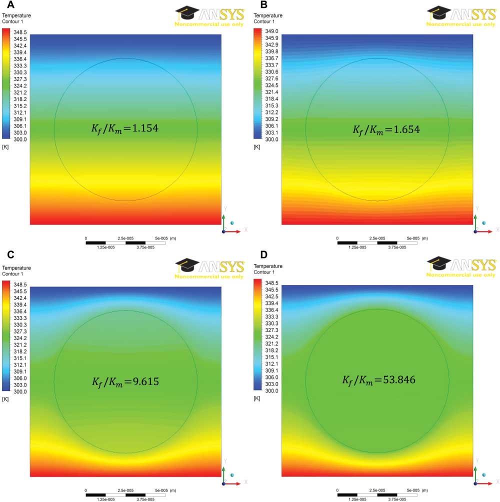
Temperature contour by CFD for four quadratic composites at Vf=0.442, ΔT=50 K: (A) cotton/air, (B) glass fibre/air, (C) nylon6/air and (D) concrete dense fibre/air.
Take nylon6/air as an example, the difference for Ke between the prediction [Eq. (13)] and the simulation is increased with the increase of Vf. Figure 9 shows the temperature contour for four Vf values under the temperature drop of 50 K. In Figure 9A, the region α shows a constant temperature gradient, while the β area demonstrates a curved temperature contour affected by Kf, indicating the variation of the local temperature gradient. The proportion of β area in the fluid is increased with increasing Vf. As shown in Figure 9C and D, the β area dominates the fluid domain, resulting in the error between the prediction and the simulation. For the fibre domain, the temperature gradient is constant at small Vf values, as shown in Figure 9A and B, giving a good agreement of prediction and simulation. However, it is clear of the curved temperature contour in the fibre of Figure 9C and D, showing a poor prediction (Figure 7C and D) based on the constant temperature gradient. A similar result was also discussed by Mogilevskaya et al. [26].
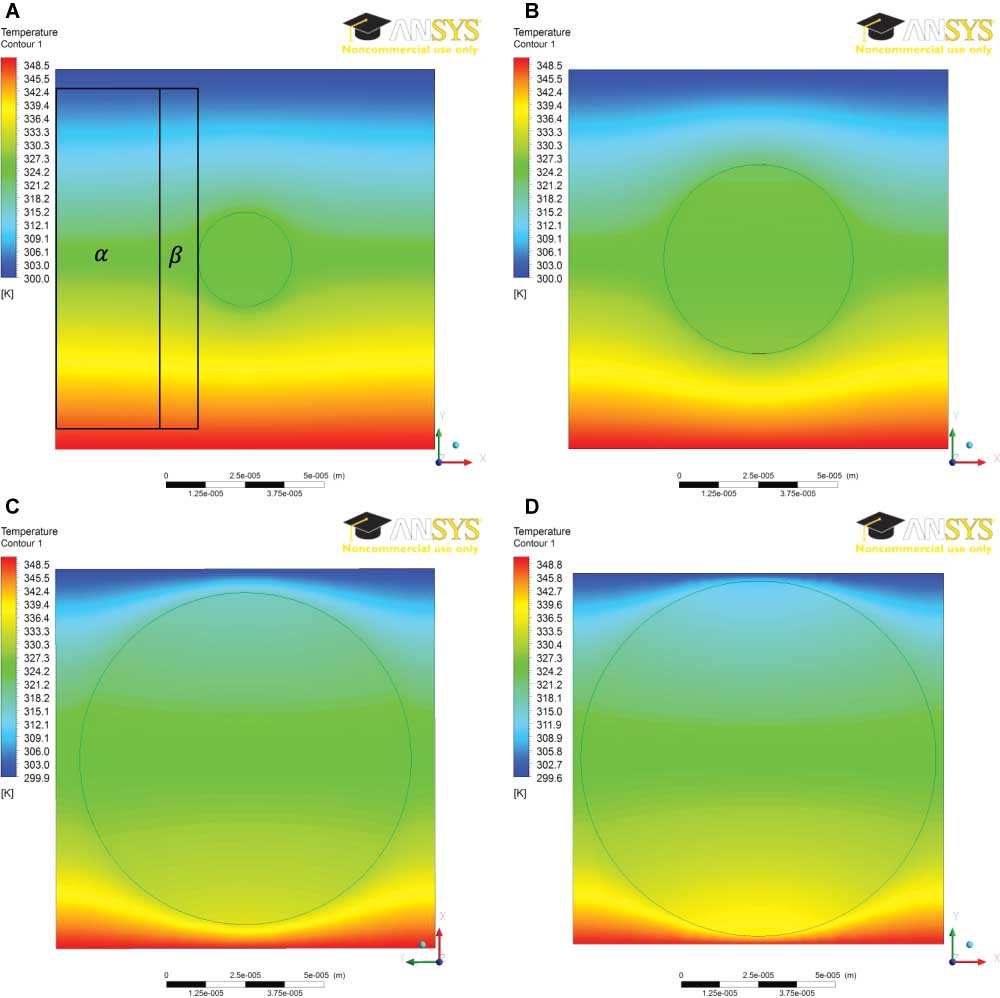
Temperature contour by CFD for the quadratic fibre array of nylon6/air, ΔT=50 K: (A) Vf=0.049, (B) Vf=0.196, (C) Vf=0.601 and (D) Vf=0.721.
3.3 Ke of hexagonal fibre array
Table 4 shows the Ke values based on CFD simulation and analytical prediction [Eqs. (4), (6), and (15)] for cotton, glass fibre, and nylon6 in air (298 K). Similar with the Ke result of quadratic fibre array, a good agreement is given between the prediction [Eq. (15)] and the simulation for hexagonal fibre array, especially when the ratio Kf/Km is close to unity. However, the reviewed models [Eqs. (4) and (6)] display better agreement with simulation than Eq. (15) when the ratio Kf/Km is increased, which is still due to the temperature gradient at the local interface.
Comparison of predictions [Eqs. (4), (6), and (15)] and simulations (CFD) for the thermal conductivity of hexagonal fibre array (Vf=0.714).
| Thermal conductivity | Eq. (4) (10-2 W/m·K) | Eq. (6) (10-2 W/m·K) | Eq. (15) (10-2 W/m·K) | Simulated data (10-2 W/m·K) |
|---|---|---|---|---|
| Cotton/air (Kf/Km=1.154) | 2.879 | 2.879 | 2.797 | 2.757 |
| Glass fibre/air (Kf/Km=1.654) | 3.709 | 3.701 | 3.353 | 3.533 |
| Nylon6/air (Kf/Km=9.615) | 9.756 | 9.438 | 6.728 | 9.263 |
3.4 Effect of thermal contact resistance
The assumption for Eqs. (13) and (15) is that there is no thermal contact resistance (Rc) at the fibre/fluid interface. However, the fibre surface is occasionally covered by a different material. For example, a heating coil is covered by a thin layer of calcium carbonate deposit. Or the interface of the fibre and resin matrix is filled with a thin layer of air. These both can give a thermal contact resistance to heat flow. On the basis of Eq. (7-3), the thermal conductivity (Kb) of the material or phase can be obtained given its thickness, contact area and resistance value. Figure 10 shows simulated Ke values of a quadratic fibre array (Vf=0.721) along Rc values. The amount of heat transfer through the interface is increased as Rc decreases. In the meantime, the temperature drop beside the interface would be smaller. Figure 10 also shows an inverse proportion of Ke and Rc, indicating a sensitive effect of Rc on the Ke of a composite.
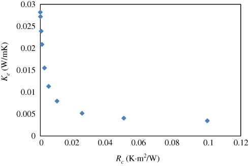
Effective thermal conductivity of cotton/air with the interface thermal contact resistance (by CFD).
Figure 11 shows the temperature contour (ΔT=50 K) for a cotton fibre in air under four Rc values. Figure 11A shows a slight undulating temperature contour for a small Rc value (10-4 K·m2/W), but the temperature drop beside the interface can be ignored. However, this becomes more evident with the increase of Rc, as shown by the temperature dislocation in Figure 11D. The resistance to heat flow at the interface causes the temperature gradient in the fibre to be much smaller compared with that in the fluid.
Temperature contour with various interface thermal contact resistance by CFD simulation for cotton/air (Vf=0.721): (A) 10-4 K·m2/W, (B) 5×10⁻⁴ K·m2/W, (C) 10-3 K·m2/W and (D) 5×10⁻³ K·m2/W.
4 Conclusions
An analytical solution was developed for predicting the effective thermal conductivity of quadratic and hexagonal fibre array impregnated in another material, such as a fluid. On the basis of electricity analogy, the model integrates the fibre and fluid thermal conductivity in parallel, and sums the rest of the fluid values in series. However, the model did not consider the deformation of temperature contour at the fibre/fluid interface.
Heat transfer through four sets of fibres in air was simulated (298 K) by CFD. Their simulated effective thermal conductivities (Ke) were compared with analytical predictions. The results showed good agreement at a small fibre volume fraction (Vf) when the fibre thermal conductivity (Kf) is close to the air value (Km). This was true for both quadratic and hexagonal fibre arrays. Temperature contour by CFD simulation showed that the ratio (Kf/Km) and Vf were key factors to an accurate analytical prediction. CFD simulation also showed that the local temperature gradient varied at the fibre/fluid interface, giving poor agreement at high Kf/Km ratio and Vf values. A larger thermal contact resistance at the fibre/fluid interface would dislocate the temperature contour, where the model fails to predict the Ke value. This would be a further investigation for this case.
The authors would like to thank ANSYS for the CFD packages. Financial assistance from the project fund RA20DV is also acknowledged.
References
[1] Springer GS, Tsai SW. J. Compos. Mater. 1967, 1, 166–173.Search in Google Scholar
[2] Hasselman DPH, Johnson LF. J. Compos. Mater. 1987, 21, 508–515.Search in Google Scholar
[3] Pitchumani R. J. Heat Transfer 1999, 121, 163–166.10.1115/1.2825931Search in Google Scholar
[4] Al-Nassar Y. Heat Mass Transf. 2006, 43, 117–122.Search in Google Scholar
[5] Wang M, He JH, Yu JY, Pan N. Int. J. Therm. Sci. 2007, 46, 848–855.Search in Google Scholar
[6] Kumlutas D, Tavman IH. J. Thermoplast. Compos. Mater. 2006, 19, 441–455.Search in Google Scholar
[7] Bailleul JL, Delaunay D, Jarny Y, Jurkowski T. J. Reinforced Plast. Compos. 2001, 20, 52–64.Search in Google Scholar
[8] Henne M, Ermanni P, Deleglise M, Krawczak P. Compos. Sci. Technol. 2004, 64, 1191–1202.Search in Google Scholar
[9] Lim TC. Mater. Lett. 2002, 54, 152–157.Search in Google Scholar
[10] Carson JK, Sekhon JP. Int. Commun. Heat Mass Transf. 2010, 37, 1226–1229.Search in Google Scholar
[11] Pan CT, Hocheng H. Compos. Part A Appl. Sci. Manuf. 2001, 32, 1657–1667.Search in Google Scholar
[12] Woodside W, Messmer JH. J. Appl. Phys. 1961, 32, 1688–1699.Search in Google Scholar
[13] Hamilton RL, Crosser OK. Ind. Eng. Chem. Fundam. 1962, 1, 187–191.Search in Google Scholar
[14] Carson JK, Lovatt SJ, Tanner DJ, Cleland AC. Int. J. Refrig. 2003, 26, 873–880.Search in Google Scholar
[15] Kulkarni MR, Brady RP. Compos. Sci. Technol. 1997, 57, 277–285.Search in Google Scholar
[16] Charles JA, Wilson DW. Polym. Compos. 1981, 2, 105–111.Search in Google Scholar
[17] Tai H. Int. J. Thermophys. 1998, 19, 1485–1492.Search in Google Scholar
[18] Zinoviev PA, Smerdov AA. Compos. Sci. Technol. 1999, 59, 625–634.Search in Google Scholar
[19] Rodriguez AC, Cabeza JMG. J. Compos. Mater. 1999, 33, 984–1001.Search in Google Scholar
[20] Cengel YA. Introduction to Thermodynamics and Heat Transfer, The McGraw-Hill Companies, Inc.: London, 1997, p. 922.Search in Google Scholar
[21] Zou MQ, Yu BM, Zhang DM. J. Phys. D Appl. Phys. 2002, 35, 1867–1874.Search in Google Scholar
[22] Rocha RPA, Cruz ME. Numer. Heat Transf. Part A Appl. 2001, 39, 179–203.Search in Google Scholar
[23] TexGen. 2011 [cited 2011 22/11]. Available from: http://texgen.sourceforge.net/index.php/Main_Page.Search in Google Scholar
[24] Altair. 2011 [cited 2011 29/11]. Available from: http://www.altairhyperworks.com/?AspxAutoDetectCookieSupport=1.Search in Google Scholar
[25] ANSYS. 2012 [cited 2012 15/05]. Available from: http://www.ansys.com/Products/Simulation+Technology/Fluid+Dynamics/ANSYS+CFX.Search in Google Scholar
[26] Mogilevskaya SG, Stolarski HK, Crouch SL. J. Mech. Phys. Solids 2012, 60, 391–417.10.1016/j.jmps.2011.12.008Search in Google Scholar
©2014 by Walter de Gruyter Berlin Boston
This article is distributed under the terms of the Creative Commons Attribution Non-Commercial License, which permits unrestricted non-commercial use, distribution, and reproduction in any medium, provided the original work is properly cited.
Articles in the same Issue
- Masthead
- Masthead
- Original articles
- New thermally stable poly(amide-imide)/montmorillonite reinforced nanocomposite based on N,N′-pyrromellitoyl-bis-l-valine: synthesis and characterization
- Thermal degradation of epoxy resin grafted with polyurethane
- Effect of single-walled carbon nanotube on the physical, rheological and mechanical properties of thermoplastic elastomer based on PP/EPDM
- Influence of ceramic particle features on the thermal behavior of PPO-matrix composites
- High-temperature mechanical behavior of Al-Cu matrix composites containing diboride particles
- Modification and adsorption performance of ultrafine iron matrix composite powder
- Densification treatment and properties of carbon fiber reinforced contact strip
- The effects of marble dust and fly ash on clay soil
- The effects of different dusty aggregate on bituminous hot mixtures
- Assessment of specific absorption rate reduction in human head using metamaterial
- Circumferential waves in pre-stressed functionally graded cylindrical curved plates
- A solution for transverse thermal conductivity of composites with quadratic or hexagonal unidirectional fibres
- Impact response of composite plates manufactured with stitch-bonded non-crimp glass fiber fabrics
- Moment methods for C/SiC woven composite components reliability and sensitivity analysis
- The effects of fabric lamination angle and ply number on electromagnetic shielding effectiveness of weft knitted fabric-reinforced polypropylene composites
- A mesh-free simulation of mode I delamination of composite structures