Bivariate traits association analysis using generalized estimating equations in family data

Mariza de Andrade; Mauricio A. Mazo Lopera; Nubia E. Duarte

doi:10.1515/sagmb-2019-0030

Article

Bivariate traits association analysis using generalized estimating equations in family data

Mariza de Andrade , Mauricio A. Mazo Lopera and Nubia E. Duarte

Published/Copyright: May 5, 2020

Published by

Become an author with De Gruyter Brill

Submit Manuscript Author Information

From the journal Statistical Applications in Genetics and Molecular Biology Volume 19 Issue 2

Abstract

Genome wide association study (GWAS) is becoming fundamental in the arduous task of deciphering the etiology of complex diseases. The majority of the statistical models used to address the genes-disease association consider a single response variable. However, it is common for certain diseases to have correlated phenotypes such as in cardiovascular diseases. Usually, GWAS typically sample unrelated individuals from a population and the shared familial risk factors are not investigated. In this paper, we propose to apply a bivariate model using family data that associates two phenotypes with a genetic region. Using generalized estimation equations (GEE), we model two phenotypes, either discrete, continuous or a mixture of them, as a function of genetic variables and other important covariates. We incorporate the kinship relationships into the working matrix extended to a bivariate analysis. The estimation method and the joint gene-set effect in both phenotypes are developed in this work. We also evaluate the proposed methodology with a simulation study and an application to real data.

Keywords: bivariate analysis; gene-set test; generalized estimating equations; family data

Corresponding author: Mariza de Andrade, Department of Health Sciences Research, Mayo Clinic, Rochester, MN, 55905, USA, E-mail: mandrade@mayo.edu

Funding source: Foundation of the São Paulo State (FAPESP)

Award Identifier / Grant number: 2007/58,150-7

Appendix A Defining the eigenvalues for the score statistic Tz distribution

Following the results of Wang et al. (2013), we denote P=∑i=1NDiTVi−1Di and partition P as Px˜x˜, Px˜z˜, Pz˜x˜ and Pz˜z˜ according to the dimensions of β and α from model (1). Let us denote Q=(Pz˜x˜Px˜x˜−1, I) and

W=∑i=1NDiTVi−1Cov(Yi)Vi−1Di

where I is the identity matrix of dimensions (2qℒ2q) and Cov(Yi) is estimated by [Yi−μ0,i][Yi−μ0,i]T, where μ0,i is obtained under the null hypothesis. When N→∞, Tz→d∑i=1qλiχi,12, where χi,12 are independent chi-squred random variables with one degree of freedom and (λ1, …, λq) are the eigenvalues of W1/2QTQW1/2, where W1/2 denotes the Cholesky decomposition of W. For more details with respect to this result see Wang et al. (2013).

Appendix B Simulating multivariate correlated phenotypes

Appendix B.1 Multivariate binary data

Let Yb,ij and Yb,ik denote two binary response variables for the j-th and k-th members of the i-th family, such that P(Yb,ij=1)=pij, P(Yb,ik=1)=pik and P(Yb,ij=1, Yb,ik=1)=pijk.

The correlation coefficient, ri,jk, for Ybij and Ybik can be written as:

rijk=pijk−pijpikpij(1−pij)pik(1−pik),

and from this equation:

(B.1)pijk=rijkpij(1−pij)pik(1−pik)+pijpik.

Given the probabilities pij and pik, and the correlation rijk, we use two latent random variables, normally distributed with variances equal to 1, Lij and Lik, to simulate Yb,ij and Yb,ik, respectively. The latent variables are obtained by equating:

pijk=P(Lij>0, Lik>0)=P(L¯ij>−μij, L¯ik>−μik),

where μij=E(Lij), μik=E(Lik), L¯ij=Lij−μij and L¯ik=Lik−μik.

Let us assume that L¯ij and L¯ik have a standard bivariate normal distribution with correlation ρijk, and joint distribution:

P(L¯ij≥a, L¯ik≥b)=∫a∞∫b∞12π(1−ρijk) exp (−lij2−2ρijklijlik+lik22(1−ρijk2))dlijdlik.

Patel and Read (1982) tabulated the values of P(L¯ij≥a, L¯ik≥b) and Leisch et al. (1998) use Monte Carlo simulations to estimate these values and provide the following algorithm to obtain the correlated binary random variables:

Choose the marginal probabilities pij and pik, and the correlation rijk.
Set μij=Φ−1(pij) and μik=Φ−1(pik), where Φ is the standard normal distribution function.
Find pijk replacing pij, pik and rijk in Eq. (B. 1).
Obtain ρijk, by equating pijk=P(L¯ij≥μij, L¯ik≥μik).
Generate the bivariate normal random variables (Lij, Lik) using the parameters μij, μik and ρijk.
Set Ybij=1⇔Lij>0 and Ybik=1⇔Lik>0.

The general process to simulate a multivariate binary random vector is available in Leisch et al. (1998) and it is implemented in the package “bindata” of R (version 3.2.2) software (Leisch et al. 2012).

Appendix B.2 Multivariate continuous data

To simulate a multivariate continuous vector, Yc, with mean μc and covariance matrix Σc, we use a vector of independent standard normal variables, u. The vector Yc is obtained using the equation:

Yc=μc+u′C,

where Σc=CC′.

Appendix B.3 Correlated multivariate continuous and binary vectors

Let Yb,ij and Yc,ik be two random variables, binary and a continuous, respectively. We have that

Cov(Yc,ik, Yb,ij)=pijE(Yc,ik|Yb,ij=1)−pijE(Yc,ik)

and from this equation

(B.2)Cov(Yc,ik, Yb,ij)pij=E(Yc,ik|Yb,ij=1)−E(Yc,ik).

On the other hand, following the ideas of Cox and Wemuth (1992),

(B.3)E(Yc,ik|Yb,ij=1)=μc,ik+Corr(Yc,ik, Lij)ψc ϕ(αc,ij)Φ(−αij)

where Lij∼N(αij, 1), Yc,ik∼N(μc,ik, ψc), αij=Φ−1(pij), μc,ik=E(Yc,ik) and

Yb,ij={1,Lij≥αij0,Lij<αij.

Replacing Eq. (B. 3) in Eq. (B. 2):

Cov(Yc,ik, Yb,ij)pij=Corr(Yc,ik, Lij)ψcϕ(αc,ij)Φ(−αij).

And thus:

Cov(Yc,ik, Yb,ij)pijℒΦ(−αij)ϕ(αc,ij)=Corr(Yc,ik, Lij)ψc=Cov(Yc,ik, Lij).

These result can be generalized for the vectors Yc,i=(Yc,i1, …, Yc,ini), Yb,i=(Yb,i1, …, Yb,ini) and Li=(Li1, …, Lini), i. e.,

(B.4)Cov(Yc,i, Li)=Cov(Yc,i, Yb,i) Di,

where

Di=diag{Φ(−αi1)pi1ℒϕ(αi1), …, Φ(−αini)piniℒϕ(αini)}.

Appendix C Pedigree for the reference families

Figure C.1 shows the pedigree graphics for the eight reference families used in the simulation study and that were obtained of the Baependi Heart Study (Oliveira et al. 2008).

Figure C.1:

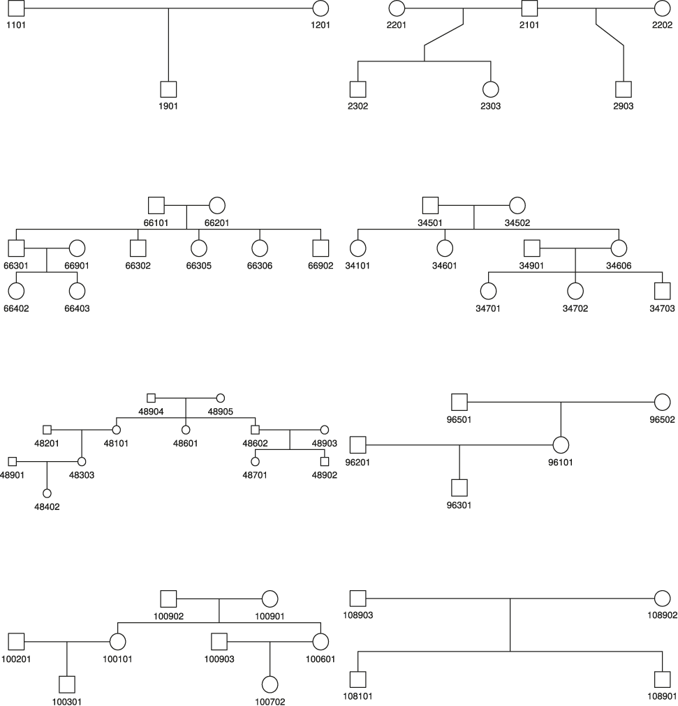
Pedigree graphics for the eight reference families used in the simulation study.

Figure C.2:

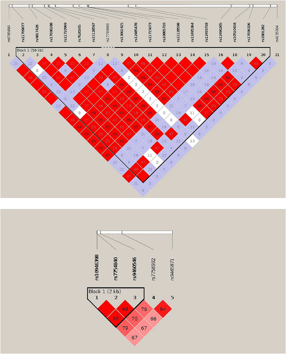
Linkage disequilibrium (LD) plot obtained from Haploview for the selected regions for PPARG (top) and CDKAL1 (bottom) SNPs of the Baependi dataset. Each diagonal represents a definite SNP and each square indicates the pairwise magnitude of LD or correlation structure between 2 SNPs corresponding to the crossing diagonals.

References

Almasy, L. and Blangero, J. (1998). Multipoint quantitative-trait linkage analysis in general pedigrees. Am. J. Hum. Genet 62: 1198–1211, https://doi.org/10.1086/301844.Search in Google Scholar

Almasy, L., Dyer, T. and Blangero, J. (1997). Bivariate quantitative trait linkage analysis: pleitropy versus co-incident linkages. Genet. Epidemiol 14: 953–958, https://doi.org/10.1002/(sici)1098-2272(1997)14:6<953::aid-gepi65>3.0.co;2-k.10.1002/(SICI)1098-2272(1997)14:6<953::AID-GEPI65>3.0.CO;2-KSearch in Google Scholar

Casale, F., Rakitsch, B., Lippert, C. and Stegle, O. (2015). Efficient set tests for the genetic analysis of correlated traits. Nat. Methods 12: 755–758, https://doi.org/10.1038/nmeth.3439.Search in Google Scholar

Cox, D. and Wemuth, N. (1992). Response models for mixed binary and quantitative variables. Biometrika 79: 441–461, https://doi.org/10.1093/biomet/79.3.441.Search in Google Scholar

de Andrade, M., Thiel, T., Yu, L. and Amos, C. (1997). Assessing linkage on chromosome 5 using components of variance approach: univariate vs. multivariate. Genet. Epidemiol 14: 773–778, https://doi.org/10.1016/J.DESAL.2008.04.014.10.1002/(SICI)1098-2272(1997)14:6<773::AID-GEPI35>3.0.CO;2-LSearch in Google Scholar

Egan, K. J., Von Schantz, M., Negrão, A., Santos, H., Horimoto, A., Duarte, N., Gonçalves, G., Soler, J., De Andrade, M., Lorenzi-Filho, G. (2016). Cohort profile: The Baependi Heart Study - A family-based, highly admixed cohort study in a rural Brazilian town. BMJ Open 6: In this issue, 1–8, https://doi.org/10.1136/bmjopen-2016-011598.Search in Google Scholar

Hopper, J. and Mathews, J. (1982). Extensions to multivariate normal models for pedigree analysis. Ann. Hum. Genet 46: 373–383, https://doi.org/10.1111/j.1469-1809.1982.tb01588.x.Search in Google Scholar

Kevin, J., Mathew, E., Qianghua, X. and Struan, F. (2014). Genetic susceptibility to type 2 diabetes and obesity: follow-up of findings from genome-wide association studies. Int. J. Endocrinol 2014: 1–13, https://doi.org/10.1155/2014/769671.Search in Google Scholar

Lange, C., Whittaker, J. and Macgregor, A. (2002). Generalized estimating equations: a hybrid approach for mean parameters in multivariate regression models. Stat. Model 2: 163–181, https://doi.org/10.1191/1471082x02st031oa.Search in Google Scholar

Lange, K. and Boehnke, M. (1983). Extensions to multivariate normal models for pedigree analysis. IV. covariance component models for multivariate traits. Am. J. Med. Genet 14: 513–524, https://doi.org/10.1002/ajmg.1320140315.Search in Google Scholar

Leal, S., Yan, K. and Muller-Myhsokb, B. (2005). SimPed: a simulation program to generate haplotype and genotype data for pedigree structures. Hum. Hered 2005: 119–122, https://doi.org/10.1159/000088914.Search in Google Scholar PubMed PubMed Central

Leisch, F., Weingessel, A. and Hornik, K. (1998). On the generation of correlated artificial binary data. Working Paper 13, SFB Adapt. Info. Syst. Model. Econ. Manag. Sci.Search in Google Scholar

Leisch, F., Weingessel, A. and Hornik, K. (2012). Bindata: generation of artificial binary data. R package version 0.9-19. Available at: http://CRAN.R-project.org/package=bindata.Search in Google Scholar

Liu, J., Pei, Y., Papasian, C. and Deng, H. (2009). Bivariate association analysis for the mixture of continuous and binary traits with the use of extended generalized estimating equations. Genet. Epidemiol 33: 217–227, https://doi.org/10.1002/gepi.20372.Search in Google Scholar PubMed PubMed Central

Oliveira, C., Pereira, A., de Andrade, M., Soler, J. and Krieger, J. (2008). Heritability of cardiovascular risk factors in a brazilian population: Baependi heart study. BMC Med. Genet 32: 1–8, https://doi.org/10.1186/1471-2350-9-32.Search in Google Scholar PubMed PubMed Central

Patel, J. and Read, C. (1982). Handbook of the normal distribution, Statistics: Textbooks and monographs, Vol. 40, 1st ed. New York an Basel: Marcel Dekker, Inc., New York.10.2307/2529920Search in Google Scholar

Pekár, S. and Brabec, M. (2018). Generalized estimating equations: a pragmatic and flexible approach to the marginal GLM modelling of correlated data in the behavioural sciences. Ethology 124: 86–93, https://doi.org/10.1111/eth.12713.Search in Google Scholar

R Core Team. (2018). R: A language and environment for statistical computing. R Foundation for Statistical Computing, Vienna, Austria. Available at: https://www.R-project.org/.Search in Google Scholar

Rochon, J. (1996). Analyzing bivariate repeated measures for discrete and continuous outcome variables. Biometrics 52: 740–750, https://doi.org/10.2307/2532914.Search in Google Scholar

Schott, J. R. (1997). Matrix analysis for statistics, 3rd ed. Wiley, New Jersey.Search in Google Scholar

Scott, L., Mohlke, K., Bonnycastle, L., Willer, C., Li, Y., Duren, W., Erdos, M., Stringham, H., Chines, P., Jackson, A., et al. (2007). A genome wide association study of type 2 diabetes in finns detects multiple susceptibility variants. Science 5829, 1341–1345, https://doi.org/10.1126/science.1142382.Search in Google Scholar PubMed PubMed Central

Turner, S., Kardia, S., Boerwinkle, E. and de Andrade, M. (2004). Multivariate linkage analysis of blood pressure and body mass index. Genet. Epidemiol 27: 64–73, https://doi.org/10.1002/gepi.20002.Search in Google Scholar PubMed

Wang, S., Meigs, J. and Dupuis, J. (2017). Joint association analysis of a binary and a quantitative trait in family samples. Eur. J. Hum. Genet 25: 130–136, https://doi.org/10.1038/ejhg.2016.134.Search in Google Scholar PubMed PubMed Central

Wang, X. (2013). gskat: GEE_KM. R package version 1.0. Available at: https://CRAN.R-project.org/package=gskat.Search in Google Scholar

Wang, X., Lee, S., Zhu, X., Redline, S. and Lin, X. (2013). GEE-based SNP set association test for continuous and discrete traits in family based association studies. Genet. Epidemiol 37: 778–786, https://doi.org/10.1002/gepi.21763.Search in Google Scholar PubMed PubMed Central

Wood, A., Tyrrell, J., Beaumont, R., Jones, S., Tuke, M., Ruth, K., Yaghootkar, H., Freathy, R., Murray, A., Frayling, T. (2016). Variants in the FTO and CDKAL1 loci have resessive effects on risk of obesity and type 2 diabetes, respectively. Diabetologia 59: 1214–1221, https://doi.org/10.1007/s00125-016-3908-5.Search in Google Scholar PubMed PubMed Central

Published Online: 2020-05-05

You are currently not able to access this content.

Articles in the same Issue

https://doi.org/10.1515/sagmb-2019-0030

Keywords for this article

bivariate analysis; gene-set test; generalized estimating equations; family data