Random forests on distance matrices for imaging genetics studies

Data sets

Concerning the simulation studies, for the purposes of realism, the simulated genotypes and quantitative phenotypes are built from the public datasets of the International HapMap Project⁷ and the Alzheimers Disease Neuroimaging Initiative (ADNI)⁸ respectively. The genotypic and phenotypic data that is used for the application on Alzheimer’s disease was also retreived from ADNI.

HapMap data

A human haplotype map of over 1.5 million SNPs for 993 subjects from 11 sub-populations across four continents was obtained from the second release of the HapMap phase 3 dataset⁹ of the International HapMap Project.

ADNI data

The ADNI study began at 2004 as a multicenter effort to develop clinical, imaging, genetic and biochemical biomarkers for the early detection and tracking of AD. The initial 6-year phase of the study (ADNI1) included 400 subjects diagnosed with mild cognitive impairment (MCI), 200 subjects with early AD and 200 elderly control subjects. In 2009, ADNI1 was extended with ADNI GO which assessed the existing ADNI1 cohort and added 200 participants identified as having early mild cognitive impairment (EMCI). Finally, in 2011, ADNI2 began, which assesses new participants in addition to those from the ADNI1/ADNI GO cohort. All participants in the ADNI studies were recruited across North America and are followed and reassessed over time to track the pathology of the disease as it progresses.

For the purpose of applying distance-based Random Forests on a real dataset, we acquired genotypes for 464 subjects from the ADNI database ((99 AD, 154 CN, 211 MCI). Genotyping was performed with the Human610-Quad Bead-Chip microarray, which includes 620,901 SNPs and copy number variations (see Saykin et al. (2010) for details). A separate genotyping of the SNPs for the APOEε4 variant has been performed by ADNI, since these were not included in the above microarray. The subjects were unrelated, of European ancestry, and passed screening for evidence of population stratification using the procedure described in Stein et al. (2010).

The selection and preprocessing steps are taken from Silver et al. (2012), where the same data was used for the identification of possible AD causal gene pathways. In detail, the genotypic data consists from autosomal SNPs with genotyping rate >95% (42,680 SNPs), HardyWeinberg equilibrium p-value >5×10⁷ and minor allele frequency >0.1. For each subject we ended up with a set of 434,271 SNPs. Any missing genotypes were imputed using the same procedure as in Vounou et al. (2012).

The imaging data consists of longitudinal brain MRI scans (1.5 T) from the ADNI database. For each of the subjects, serial brain MR images were acquired at baseline and at 6, 12 and 24 months following initial recruitment. Details about the acquisition protocol and the preprocessing steps that were applied by ADNI on the raw scans can be found in Jack et al. (2008).

Further processing was carried out, as described in detail in Silver et al. (2012). The aim is to provide a measure of brain structural change over time. To achieve that, a linear regression model with an intercept term and time as the independent variable is fitted for each voxel. The coefficient for the slope provides a measure of brain tissue change, relative to time, for each voxel. Correction for age and sex, as well as selection of the most discriminative voxels is performed by analysis of variance (ANOVA) (Silver et al., 2012). The final endophenotype data that we use is in the form of longitudinal maps of ventricular/CSF expansion (reconstructed to 1 mm isotropic voxels), which represent brain tissue loss and are normalised across all the subjects. Each subject’s endophenotype vector consists of 148,023 slope coefficients.

The simulation studies below were performed using information from the subset of CN and AD subjects, while for the application study, MCI subjects were included as well.

Imaging genetics simulation engine

In this section we provide details of the imaging genetics simulation engine. We describe, in order, the genotype simulation, the phenotype simulation, the genetic disease modelling, and lastly the disease classification modelling.

Base genotype simulation

The ADNI dataset with 253 subjects is clearly too small to represent a direct population source for the multiple samples required for the multiple simulation runs. Instead we simulate this base population and its genotype within an individual-based, forward-time, population genetics simulation environment. Specifically we employed the SimuPOP Python package (Peng and Kimmel, 2005) and have made use of the SimuGWAS¹⁰ implementation (Peng and Amos, 2010), originally written for the simulation of samples for GWAS studies. This allows one to evolve the genotype of a given starting population over a specified number of generations with exposure to the standard evolutionary forces of mutation, recombination, migration, and selection.

The pattern of linkage disequilibrium (LD) between markers in a forward-time simulated population is sensitive to the make-up of the starting population. In the absence of data on populations in the distant past, we adopt the HapMap phase 3 subjects as a reasonable proxy. Rather than evolving the entire genotype, it is suffices for our simulation study to restrict our attention to a subset of genetic markers located on a single chromosome. From all 993 subjects in the HapMap dataset, we extract 385 sequential, biallelic, SNP markers from the front end of chromosome 19 with a minimum maf of 0.05. We perform a forward-time evolution of this initial population of 993 individuals over 500 non-overlapping generations using the Wright-Fisher model. We assume a constant population growth rate towards a final population of 10000 individuals. We maintain a recombination rate of 1.0×10^–8, a mutation rate of 1.0×10^–8, and a migration rate of 1.0×10^–3 throughout the simulated evolutionary process.

We denote the genotype of individual i at locus s by the minor allele count x_is∈{0, 1, 2}. From the set of 385 markers, we identify two subsets of 16 SNPs with maf~0.2,¹¹ the purpose of which will be made explicit later in Section 6. Let the two subsets be S_c and S_s, where the subscripts indicate the labels potentially causative and potentially spurious respectively. We emphasise the potentiality in their descriptions to highlight the fact that, depending on the specific genetic model simulated (see later), not all the SNPs from the two sets will be associated to phenotypic modifications.

We consider a single chromosome with 385 markers and denote the genotype of individual i at locus s by the minor allele count x_is∈{0, 1, 2}. We assign two subsets of SNPs, S_c and S_s, which we label potentially causative and potentially spurious respectively. We emphasise the potentiality in their descriptions to highlight the fact that, depending on the specific genetic model simulated (see later), not all the SNPs from the two sets will be associated to phenotypic modifications.

Base phenotype simulation

There is no constraint on the number or type of imaging phenotypes for the simulation model. In this paper we consider two such quantitative phenotypes – a multivariate, vectorial, representation and a matrix representation of imaging phenotypes. These representations are motivated by both the neuroimaging data currently available, and also by the pathology of AD. For instance, the neuronal atrophy in AD patients can be represented as vector of time-averaged rates of volume change of the various ROIs in the brain. Also, as demonstrated in several more recent studies (Sun et al., 2009; Huang et al., 2010; Brier et al., 2012), the number of connections between different ROI is shown to be lower in AD subjects as compared with CN subjects. A similar decrease in connectivity is also observed in longitudinal FDG-PET and resting-state functional MRI (rs-fcMRI) scans of individual AD subjects (Sun et al., 2009; Brier et al., 2012). Although there are exceptions at the beginning of AD progression where connections between certain brain regions increase, it is believed that such localised changes are simply compensatory responses to the overall decline in brain connectivity. As the disease progresses, the exceptional trends reverts to the global pattern of a decrease in connectivity. Therefore, for the second endophenotype, we consider a matrix-valued phenotype representing brain-networks.

We denote the base vectorial phenotype of the kth ROI of individual i by y_ik. Although we generate these vectors from the ADNI data representing voxel-wise ventricular volume expansion rates, the simulation framework is not dependent on the chosen method; indeed any suitable method for generating realistic vectors representing alternative imaging phenotypes is entirely permissible.

We plot the linear regression slope coefficient of the ventricular volume against time and identify, for the 253 ADNI subjects, a 148023-voxel subset of the full-brain MRI scan which is maximally discriminative between AD and CN. Given that we aim to perform multiple RF runs over multiple scenarios, we perform a simple k-means clustering, transforming the 148023-voxel ventricular volume gradients to that of just 400 parcels, simulating a lower-resolution image. This choice is arbitrary except for the fact that it is larger than the sample size, thereby simulating a large-p/small-N scenario.

For each individual in our simulated population, the aim is simply to generate a 400-dimensional vectorial phenotype to represent the base ventricular gradients of the 400 ROIs on which the genetic model modifications can be imputed. We require, for realism, that after implementing the genetic modifications, the multivariate distribution of this phenotype resembles the empirical distribution of the subjects from the ADNI dataset. The practical implementation of the base ventricular volumes is performed in two steps, as follows.

For the first step, we generate random samples from a multivariate Gaussian distribution where the mean and covariance matrix parameters are taken from the sample mean and sample covariance matrix of the 154 CN subjects. Note that because there are fewer subjects than ROIs (154<400), the sample covariance matrix is unstable, requiring, therefore, the use of a James-Stein-type shrinkage estimator (Schäfer and Strimmer, 2005) for the covariance matrix. The distribution of rate gradients across all parcels of cognitive normal (CN) subjects has an average and standard deviation of –0.38 and 2.27 respectively, reflecting an overall decrease and variability in ventricular volume gradients in the base population across all the parcels. We denote the imaging trait of the kth ROI of individual i by y_ik.

For the second step, in anticipation of our genetic effects model where an overall increase in each vector component is observed, we modify the above random samples by reducing the gradient for selected ROIs. As shown in (Silver et al., 2012), the brain matter atrophy is not uniform throughout the brain. We simulate this effect by selecting a subset of n_d=28 randomly selected ROIs which we label disease-affected-ROIs, which corresponds to regions affected by selected SNPs which, in turn, has a measurable on the disease status. We label the ROI-index subset by R_d. Therefore the modification in this second step is

where ζ>0 is a parameter which is tuned according to the disease model (see below).

It is not unreasonable to assume that the volumes, and by extension the rate of volumetric changes, of functionally interconnected brain regions correlate positively (McAlonan et al., 2005). This link between structural and functional aspects can be used to indirectly estimate brain connectivity networks via the atrophy gradients. We simulate the brain connectivity by first considering the full (non-partial) correlations between the same 400 ROI. From the n_CN=154 subjects, we have the empirical covariance matrix

We generate the base covariance matrices for each of our 200 subjects by introducing random perturbations from the unit Normal at each component

with for subject i. We symmetrise the resulting matrix ensuring that it remains positive definite (Higham, 2002).

The graph representation of the network is inferred by identically matching the zero-components of the adjacency matrix of G_i with the zeros of the the sparse inverse covariance estimate (SICE) of (Sun et al., 2009; Huang et al., 2010). Let Θ⁽ⁱ⁾=(Σ⁽ⁱ⁾)^–1 be the inverse covariance matrix. Assuming that the observations follow a multivariate Gaussian, the SICE is obtained by maximising over Θ the L₁-penalised log-likelihood,

where ||Θ||₁ is the sum over the absolute values of all elements in Θ. We use the graphical lasso algorithm (Friedman et al., 2008) to estimate Σ, and hence Θ. The regularisation parameter is set as ρ=1 throughout.

One example of such a simulated brain network in the context on AD is found in Sun et al. (2009) where the authors used the SICE approach on FDG-PET data to uncover connectivity among different brain regions.

The brain connectivity network of each subject is represented by a 400-dimensional square matrix, representing either the covariance between the different ROIs or the adjacency matrix of a 400-node graph. In this paper we consider both cases. The covariance and adjacency matrices are written as and G_i respectively.

Genetic disease modelling

The second step in our simulations is the construction of the disease models. There are two aspects to this – the genetic effects on the endophenotypes, which includes both disease-related and “spurious” non-disease related effects, and the disease classification model.

Let y_β be the simulated baseline vectorial phenotype at the ROI with index β. We assume a simple additive genetic model where the components of the vector modified from the base value are given by

where the effect size w_β is built from multiplicative interaction effects as

P_‧ refers to the interaction causal models above, and x_a={0, 1, 2} is the minor allele frequency at locus a, etc. δ_β is an effect-size parameter which, when increased, with all else equal, monotonically boosts the population disease penetrance levels (see Disease classification models below). For simplicity, we fix δ_β=δ for all affected ROI.

In selected simulation runs, we include the presence of “spurious” SNP pairs and brain ROI (see Figure 2). These are labelled “spurious” because the genetic effects on the brain phenotype do not affect the propensity to develop the disease of interest. In our simulations, we assume that these do not overlap with their “causal” counterparts. Using the identical tuning parameter δ we employ a similar genetic effects model as above.

For the changes to brain networks, we propose an additive genetic model, similar to (24) where the strength of correlations between different ROI is scaled with a simple exponential factor. Let be the covariance matrix representing the brain connectivity. The components of the attenuated representative covariance matrix Σ′* are given by

where γ>0 is the effect-size parameter. In this model, both positive and negative correlations between different brain regions are reduced in magnitude.

The final piece in the imaging genetics simulation engine is the method for assigning a case-control disease status to each subject. This serves the following two purposes. It allows us to establish the power of imaging genetics via a comparison of quantitative vs. case-control RF regressions, and it is used to validate the supervised learning approach to define distances between brain networks.

To minimise the model complexity, we only consider the effects of the increase in vectorial phenotype on the disease classification, neglecting the contribution of the decrease in brain connectivity. Given that a correlation between structural and functional connectivity is built in into our simulations, this is not an unreasonable simplification.

Based on empirical observations of the ADNI data, we have the following design considerations for constructing an AD disease classification model. Firstly, such a model is inherently probabilistic with the propensity to develop AD increasing with the overall ventricular volume gradient of a sub-region of the whole brain. Analysis of the ADNI data in Silver et al. (2012) suggests that this highly discriminating region is made up of ~7% of the total brain area; this corresponds, in our simulation set-up of 400 parcels, to 28 ROI. Secondly, as already mentioned, the distribution of volume gradients in the output of such a model, for both AD and CN classes, must agree with the empirical conditional probability distributions from the ADNI data. Thirdly, the model should allow for a range AD population penetrance values which can be set independently of the effect size. We propose, therefore, the following simple, semi-empirical, Bayesian probability model for AD classification based on the average gradient of the causal region R_d.

Let the represent the average gradient of the causal region R_d for a given subject i, i.e.,

where n_d=28 in this simulation set-up, and the * symbolises the values post-genetic effects. Let the disease status be wholly determined by i.e., we have the following equivalence between conditional probabilities for a subject i begin given an AD classification

where z_i=1, 0 are the AD/CN classification label for subject i respectively. Using Bayes’s Theorem, we write

where p(z_i=1) is the AD population penetrance level. The likelihoods and are empirically determined from the ADNI data. As before, we assume a Gaussian distribution in the ADNI data, with the sample means and for the CN and AD classes respectively. To avoid the situation where the probability of a AD classification given a large, negative, is greater than the probability of a CN classification, and vice versa, we assume that the variances of the normal distributions, representing the respective likelihoods of the CN/AD classes, are identical. We therefore take the average of the two standard deviations, i.e., In Figure 13 we show the empirically determined AD classification probability (28) as a function of for several different AD population penetrance levels.

Figure 13

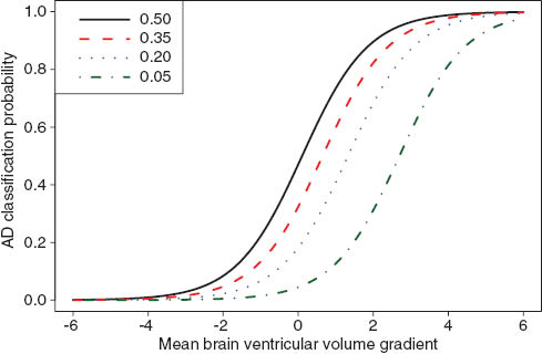
The empirical AD classification probability as a function of mean brain ventricular volume gradient. The individual curves (green, blue, red, and black) represent a range of AD population penetrance levels (5%, 20%, 35%, and 50% respectively).

References

Albert, M. S., S. T. DeKosky, D. Dickson, B. Dubois, H. H. Feldman, N. C. Fox, A. Gamst, D. M. Holtzman, W. J. Jagust, R. C. Petersen, P. J. Snyder, M. C. Carrillo, B. Thies and C. H. Phelps (2011): “The diagnosis of mild cognitive impairment due to Alzheimer’s disease: recommendations from the National Institute on Aging-Alzheimer’s Association workgroups on diagnostic guidelines for Alzheimer’s disease,” Alzheimers Dement.: J. Alzheimer’s Assoc., 7, 270–279.Suche in Google Scholar
Alter, M. D., R. Kharkar, K. E. Ramsey, D. W. Craig, R. D. Melmed, T. A. Grebe, R. C. Bay, S. Ober-Reynolds, J. Kirwan, J. J. Jones, J. B. Turner, R. Hen and D. A. Stephan (2011): “Autism and Increased Paternal Age Related Changes in Global Levels of Gene Expression Regulation,” PLOS One, 6 (2), e16715.10.1371/journal.pone.0016715Suche in Google Scholar PubMed PubMed Central
Belkin, M. and P. Niyogi (2003): “Laplacian Eigenmaps for Dimensionality Reduction and Data Representation,” Neural. Comput., 15, 1373–1396.Suche in Google Scholar
Braak, H. H. and E. E. Braak (1998): “Evolution of neuronal changes in the course of Alzheimer’s disease,” J. Neural Transm. Supplementum, 53, 127–140.Suche in Google Scholar
Breiman, L. (1984): Classification and regression trees, US, Florida: Chapman & Hall/CRC.Suche in Google Scholar
Breiman, L. (2001): “Random forests - Springer,” Mach. Learn., 45, 5–32.Suche in Google Scholar
Brier, M. R., J. B. Thomas, A. Z. Snyder, T. L. Benzinger, D. Zhang, M. E. Raichle, D. M. Holtzman, J. C. Morris and B. M. Ances (2012): “Loss of intranetwork and internetwork resting state functional connections with Alzheimer’s disease progression,” J. Neurosci., 32, 8890–8899.Suche in Google Scholar
Bureau, A., J. Dupuis, K. Falls, K. Lunetta, B. Hayward, T. Keith and P. Van Eerdewegh (2005): “Identifying SNPs predictive of phenotype using random forests,” Genet. Epidimiol., 28, 171–182.Suche in Google Scholar
Busoniu, L., R. Babuska, B. De Schutter and D. Ernst (2010): “Extremely randomized trees,” in Reinforcement learning and dynamic programming using function approximations, Automation and Control Engineering Series, Florida, US: CRC Press-Taylor & Francis Group, pp. 235–238.Suche in Google Scholar
Chen, L., G. Yu, C. D. Langefeld, D. J. Miller, R. T. Guy, J. Raghuram, X. Yuan, D. M. Herrington and Y. Wang (2011): “Comparative analysis of methods for detecting interacting loci,” BMC Genomics, 12, Article no. 344.Suche in Google Scholar
Corder, E. H., A. M. Saunders, W. J. Strittmatter, D. E. Schmechel, P. C. Gaskell, G. W. Small, A. D. Roses, J. L. Haines and M. A. Pericak-Vance (1993): “Gene dose of apolipoprotein E type 4 allele and the risk of Alzheimer’s disease in late onset families,” Science (New York, N.Y.), 261, 921–923.Suche in Google Scholar
Criminisi, A. (2012): “Decision forests: a unified framework for classification, regression, density estimation, manifold learning and semi-supervised learning,” Foundations and Trends in Computer Graphics and Vision, 7, 81–227.10.1561/0600000035Suche in Google Scholar
Deza, M.-M. and E. Deza (2013): “Encyclopedia of Distances,” Springer-Verlag, ISBN 978-3-642-00233-5.10.1007/978-3-642-30958-8Suche in Google Scholar
De Lobel, L., P. Geurts, G. Baele, F. Castro-Giner, M. Kogevinas and K. Van Steen (2010): “A screening methodology based on Random Forests to improve the detection of gene-gene interactions,” Eur. J. Hum. Genet., 18, 1127–1132.Suche in Google Scholar
Drzezga, A., T. Grimmer, G. Henriksen, I. Stangier, R. Pemeczky, J. Diehl-Schmid, C. A. Mathis, W. E. Klunck, J. Price, S. DeKosky, H.-J. Wester, M. Schwaiger and A. Kurz (2008): “Imaging of amyloid plaques and cerebral glucose metabolism in semantic dementia and Alzheimer’s disease,” NeuroImage, 39, 619–633.10.1016/j.neuroimage.2007.09.020Suche in Google Scholar PubMed
Förstner, W. and B. Moonen (1999): “A metric for covariance matrices,” Quo vadis geodesia, 113–.Suche in Google Scholar
Friedman, J., T. Hastie and R. Tibshirani (2008): “Sparse inverse covariance estimation with the graphical lasso.” Biostatistics (Oxford, England), 9, 432–441.10.1093/biostatistics/kxm045Suche in Google Scholar PubMed PubMed Central
Gerber, S., T. Tasdizen, S. Joshi and R. Whitaker (2009): “On the manifold structure of the space of brain images,” Med. Image Comput. Comput. Assist. Interv., 12, 305–312.Suche in Google Scholar
Gerber, S., T. Tasdizen, P. Thomas Fletcher, S. Joshi and R. Whitaker (2010): “Manifold modeling for brain population analysis,” Med. Image Anal., 14, 643–653.Suche in Google Scholar
Glahn, D. C., P. M. Thompson and J. Blangero (2007): “Neuroimaging endophenotypes: strategies for finding genes influencing brain structure and function,” Hum. Brain Mapp., 28, 488–501.Suche in Google Scholar
Goldstein, B. A., A. E. Hubbard, A. Cutler and L. F. Barcellos (2010): “An application of Random forests to a genome-wide association dataset: methodological considerations & new findings,” BMC Genetics, 11, Article no. 49.Suche in Google Scholar
Goldstein, B. A., E. C. Polley and F. B. S. Briggs (2011): “Random forests for genetic association studies,” Statis. Appl. Genetics Mol. Biol., 10, 32.Suche in Google Scholar
Gray, K. R., P. Aljabar, R. A. Heckemann, A. Hammers, D. Rueckert and for the Alzheimer’s Disease Neuroimaging Initiative (2013): “Random forest-based similarity measures for multi-modal classification of Alzheimer’s disease,” Neuroimage, 65C, 167–175.10.1016/j.neuroimage.2012.09.065Suche in Google Scholar PubMed PubMed Central
Gray, K. R., P. Aljabar, R. A. Heckemann, A. Hammers and D. Rueckert (2011): Random forest-based manifold learning for classification of imaging data in dementia. In: Machine Learning in Medical Imaging, Berlin, Heidelberg: Springer Berlin Heidelberg, pp. 159–166.10.1007/978-3-642-24319-6_20Suche in Google Scholar
Hahn, L., M. Ritchie and J. Moore (2003): “Multifactor dimensionality reduction software for detecting gene-gene and gene-environment interactions,” Bioinformatics, 19, 376–382.10.1093/bioinformatics/btf869Suche in Google Scholar PubMed
Hastie, T., R. Tibshirani and J. Friedman (2009): The elements of statistical learning, Springer Series in Statistics, second edition, New York: Springer.10.1007/978-0-387-84858-7Suche in Google Scholar
Higham, N. J. (2002): “Computing the nearest correlation matrix–a problem from finance,” IMA J. Numer. Anal., 22, 329–343.Suche in Google Scholar
Hinrichs, C., V. Singh, G. Xu and S. C. Johnson (2011): “Predictive markers for AD in a multi-modality framework: an analysis of MCI progression in the ADNI population,” Neuroimage, 55, 16–16.10.1016/j.neuroimage.2010.10.081Suche in Google Scholar PubMed PubMed Central
Huang, S., J. Li, L. Sun, J. Ye, A. Fleisher, T. Wu, K. Chen and E. Reiman (2010): “Learning brain connectivity of Alzheimer’s disease by sparse inverse covariance estimation,” Neuroimage, 50, 935–949.10.1016/j.neuroimage.2009.12.120Suche in Google Scholar PubMed PubMed Central
Iwamoto, K., M. Bundo and T. Kato (2005): “Altered expression of mitochondria-related genes in postmortem brains of patients with bipolar disorder or schizophrenia, as revealed by large-scale DNA microarray analysis,” Hum. Mol. Genet., 14, 241–253.10.1093/hmg/ddi022Suche in Google Scholar PubMed
Iwangoff, P., R. Armbruster, A. Enz and W. Meierruge (1980): “Glycolytic Enzymes from human autoptic brain cortex - normal aged and demented cases,” Mech. Ageing Deve., 14, 203–209.Suche in Google Scholar
Jack, C. R., Jr., M. A. Bernstein, N. C. Fox, P. Thompson, G. Alexander, D. Harvey, B. Borowski, P. J. Britson, J. L. Whitwell, C. Ward, A. M. Dale, J. P. Felmlee, J. L. Gunter, D. L. G. Hill, R. Killiany, N. Schuff, S. Fox-Bosetti, C. Lin, C. Studholme, C. S. DeCarli, G. Krueger, H. A. Ward, G. J. Metzger, K. T. Scott, R. Mallozzi, D. Blezek, J. Levy, J. P. Debbins, A. S. Fleisher, M. Albert, R. Green, G. Bartzokis, G. Glover, J. Mugler, M. W. Weiner and A. Study (2008): “The Alzheimer’s Disease Neuroimaging Initiative (ADNI): MRI methods,” J. Magn. Reson. Im., 27, 685–691.Suche in Google Scholar
Jiang, R., W. Tang, X. Wu and W. Fu (2009): “A random forest approach to the detection of epistatic interactions in case-control studies,” BMC Bioinformatics, 10. doi: 10.1186/1471-2105-10-S1-S65.10.1186/1471-2105-10-S1-S65Suche in Google Scholar PubMed PubMed Central
Kohannim, O., D. P. Hibar, J. L. Stein, N. Jahanshad, C. R. Jack, Jr., M. W. Weiner, A. W. Toga, P. M. Thompson and A. D. N. Initiative (2011): “Boosting power to detect genetic associations in imaging multi-locus, genome-wide scans and ridge regression,” In: 2011 8th IEEE International Symposium on Biomedical Imaging (ISBI) - From Nano to Macro, pp. 1855–1859.Suche in Google Scholar
Marchini, J., P. Donnelly and L. Cardon (2005): “Genome-wide strategies for detecting multiple loci that influence complex diseases,” Nat. Genet., 37, 413–417.Suche in Google Scholar
McAlonan, G. M., V. Cheung, C. Cheung, J. Suckling, G. Y. Lam, K. S. Tai, L. Yip, D. G. M. Murphy and S. E. Chua (2005): “Mapping the brain in autism. A voxel-based MRI study of volumetric differences and intercorrelations in autism,” Brain: A J. Neurol., 128, 268–276.Suche in Google Scholar
McKinney, B. A., J. E. Crowe, Jr., J. Guo and D. Tian (2009): “Capturing the spectrum of interaction effects in genetic association studies by simulated evaporative cooling network analysis,” PLOS Genetics, 5 (3).10.1371/journal.pgen.1000432Suche in Google Scholar PubMed PubMed Central
Miller, D. J., Y. Zhang, G. Yu, Y. Liu, L. Chen, C. D. Langefeld, D. Herrington and Y. Wang (2009): “An algorithm for learning maximum entropy probability models of disease risk that efficiently searches and sparingly encodes multilocus genomic interactions,” Bioinformatics (Oxford, England), 25, 2478–2485.10.1093/bioinformatics/btp435Suche in Google Scholar PubMed PubMed Central
Minas, C., S. J. Waddell and G. Montana (2011): “Distance-based differential analysis of gene curves.” Bioinformatics (Oxford, England), 27, 3135–3141.10.1093/bioinformatics/btr528Suche in Google Scholar PubMed
Moosmann, F., B. Triggs, F. Jurie (2007): “Fast discriminative visual codebooks using randomized clustering forests,” Adv. Neural Info. Processing Syst. 19, 985–992.Suche in Google Scholar
Pedregosa, F., G. Varoquaux, A. Gramfort, V. Michel, B. Thirion, O. Grisel, M. Blondel, P. Prettenhofer, R. Weiss, V. Dubourg, J. Vanderplas, A. Passos, D. Cournapeau, M. Brucher, M. Perrot and E. Duchesnay (2011): “Scikit-learn: Machine learning in python,” J. Mach. Learn. Res., 12, 2825–2830.Suche in Google Scholar
Peng, B. B. and M. M. Kimmel (2005): “simuPOP: A forward-time population genetics simulation environment.” Bioinformatics (Oxford, England), 21, 3686–3687.10.1093/bioinformatics/bti584Suche in Google Scholar PubMed
Peng, B. and C. I. Amos (2010): “Forward-time simulation of realistic samples for genome-wide association studies,” BMC Bioinformatics, 11, 442–442.10.1186/1471-2105-11-442Suche in Google Scholar PubMed PubMed Central
Pericak-Vance, M., J. Bebout, P. Gaskell, L. Yamaoka, W. Hung, A. MJ, A. Walker, R. Bartlett, C. Haynes, K. Welsh, N. Earl, A. Heyman, C. Clark and A. Roses (1991): “Linkage studies in Familiar Alzheimer-disease - Evidence for Chromosome 19 linkage,” Am. J. Hum. Genet., 48, 1034–1050.Suche in Google Scholar
Saykin, A. J., L. Shen, T. M. Foroud, S. G. Potkin, S. Swaminathan, S. Kim, S. L. Risacher, K. Nho, M. J. Huentelman, D. W. Craig, P. M. Thompson, J. L. Stein, J. H. Moore, L. A. Farrer, R. C. Green, L. Bertram, C. R. Jack, Jr., M. W. Weiner and A. D. N. Initi (2010): “Alzheimer’s Disease Neuroimaging Initiative biomarkers as quantitative phenotypes: genetics core aims, progress, and plans,” Alzheimer’s Dement.: J. Alzheimer’s Assoc., 6, 265–273.Suche in Google Scholar
Schäfer, J. and K. Strimmer (2005): “A shrinkage approach to large-scale covariance matrix estimation and implications for functional genomics.” Stat. Appl. Genet. Mol. Biol., 4 (1), Article no. 32.10.2202/1544-6115.1175Suche in Google Scholar PubMed
Scherzer, C. R., A. C. Eklund, L. J. Morse, Z. Liao, J. J. Locascio, D. Fefer, M. A. Schwarzschild, M. G. Schlossmacher, M. A. Hauser, J. M. Vance, L. R. Sudarsky, D. G. Standaert, J. H. Growdon, R. V. Jensen and S. R. Gullans (2007): “Molecular markers of early Parkinson’s disease based on gene expression in blood,” Proc. Nat. Acad. Sci. USA, 104, 955–960.10.1073/pnas.0610204104Suche in Google Scholar PubMed PubMed Central
Segal, M. and Y. Xiao (2011): “Multivariate random forests,” Wiley Interdisciplinary Reviews: Data Mining and Knowledge Discovery, 1, 80–87.10.1002/widm.12Suche in Google Scholar
Silver, M., E. Janousova, X. Hua, P. M. Thompson, G. Montana and The Alzheimer’s Disease Neuroimaging Initiative (2012): “Identification of gene pathways implicated in Alzheimer’s disease using longitudinal imaging phenotypes with sparse regression,” Neuroimage, 63, 1681–1694.10.1016/j.neuroimage.2012.08.002Suche in Google Scholar PubMed PubMed Central
Sperling, R. A., P. S. Aisen, L. A. Beckett, D. A. Bennett, S. Craft, A. M. Fagan, T. Iwatsubo, C. R. Jack, J. Kaye, T. J. Montine, D. C. Park, E. M. Reiman, C. C. Rowe, E. Siemers, Y. Stern, K. Yaffe, M. C. Carrillo, B. Thies, M. Morrison-Bogorad, M. V. Wagster and C. H. Phelps (2011): “Toward defining the preclinical stages of Alzheimer’s disease: recommendations from the National Institute on Aging-Alzheimer’s Association workgroups on diagnostic guidelines for Alzheimer’s disease,” Alzheimer’s Dement.: J. Alzheimer’s Assoc., 7 (3), 280–292.10.1016/j.jalz.2011.03.003Suche in Google Scholar PubMed PubMed Central
Stein, J. L. J., X. X. Hua, S. S. Lee, A. J. A. Ho, A. D. A. Leow, A. W. A. Toga, A. J. A. Saykin, L. L. Shen, T. T. Foroud, N. N. Pankratz, M. J. M. Huentelman, D. W. D. Craig, J. D. J. Gerber, A. N. A. Allen, J. J. J. Corneveaux, B. M. B. Dechairo, S. G. S. Potkin, M. W. M. Weiner and P. P. Thompson (2010): “Voxelwise genome-wide association study (vGWAS),” Neuroimage, 53, 15.10.1016/j.neuroimage.2010.02.032Suche in Google Scholar PubMed PubMed Central
Strittmatter, W. J., A. M. Saunders, D. Schmechel, M. Pericak-Vance, J. Enghild, G. S. Salvesen and A. D. Roses (1993): “Apolipoprotein E: high-avidity binding to beta-amyloid and increased frequency of type 4 allele in late-onset familial Alzheimer disease,” Proc. Natl. Acad. Sci. USA, 90, 1977–1981.10.1073/pnas.90.5.1977Suche in Google Scholar PubMed PubMed Central
Sun, L., R. Patel, J. Liu, K. Chen, T. Wu, J. Li, E. Reiman and J. Ye (2009): “Mining brain region connectivity for Alzheimer’s disease study via sparse inverse covariance estimation,” in the 15th ACM SIGKDD international conference, New York, USA: ACM Press, 1335.10.1145/1557019.1557162Suche in Google Scholar
Tenenbaum, J. B., V. de Silva and J. C. Langford (2000): “A global geometric framework for nonlinear dimensionality reduction,” Science, 290, 2319–2323.10.1126/science.290.5500.2319Suche in Google Scholar PubMed
Verma, R., P. Khurd and C. Davatzikos (2007): “On analyzing diffusion tensor images by identifying manifold structure using isomaps,” IEEE Trans. Med. Imaging, 26, 772–778.10.1109/TMI.2006.891484Suche in Google Scholar PubMed
Vounou, M., E. Janousova, R. Wolz, J. L. Stein, P. M. Thompson, D. Rueckert, G. Montana and Alzheimer’s Disease Neuroimaging Initiative (2012): “Sparse reduced-rank regression detects genetic associations with voxel-wise longitudinal phenotypes in Alzheimer’s disease,” Neuroimage, 60, 700–716.10.1016/j.neuroimage.2011.12.029Suche in Google Scholar PubMed PubMed Central
Vounou, M., T. E. Nichols and G. Montana (2010): “Discovering genetic associations with high-dimensional neuroimaging phenotypes: a sparse reduced-rank regression approach,” Neuroimage, 53, 1147–1159.10.1016/j.neuroimage.2010.07.002Suche in Google Scholar PubMed PubMed Central
Warde-Farley, D., S. L. Donaldson, O. Comes, K. Zuberi, R. Badrawi, P. Chao, M. Franz, C. Grouios, F. Kazi, C. T. Lopes, A. Maitland, S. Mostafavi, J. Montojo, Q. Shao, G. Wright, G. D. Bader and Q. Morris (2010): “The GeneMANIA prediction server: biological network integration for gene prioritization and predicting gene function,” Nucleic Acid Res., 38, W214–W220.Suche in Google Scholar
Yang, C., Z. He, X. Wan, Q. Yang, H. Xue and W. Yu (2009): “SNPHarvester: a filtering-based approach for detecting epistatic interactions in genome-wide association studies,” Bioinformatics, 25, 504–511.10.1093/bioinformatics/btn652Suche in Google Scholar PubMed
Yoshida, M. and A. Koike (2011): “SNPInterForest: a new method for detecting epistatic interactions,” BMC Bioinformatics, 12, Article no. 469.Suche in Google Scholar
Zhang, D., Y. Wang, L. Zhou, H. Yuan and D. Shen (2011): “Multimodal classification of Alzheimer’s disease and mild cognitive impairment,” NeuroImage, 55, 856–867.10.1016/j.neuroimage.2011.01.008Suche in Google Scholar PubMed PubMed Central
Zhang, Y. and J. S. Liu (2007): “Bayesian inference of epistatic interactions in case-control studies,” Nat. Genet., 39, 1167–1173.Suche in Google Scholar
Zhang, Y., D. J. Miller, and G. Kesidis (2009): “Hierarchical maximum entropy modeling for regression,” In: 2009 IEEE International Workshop on Machine Learning for Signal Processing (MLSP), IEEE, 1–6.10.1109/MLSP.2009.5306225Suche in Google Scholar
Zhao, W.-Q., P. N. Lacor, H. Chen, M. P. Lambert, M. J. Quon, G. A. Krafft and W. L. Klein (2009): “Insulin receptor dysfunction impairs cellular clearance of neurotoxic oligomeric a beta,” J. Biol. Chem., 284, 18742–18753.Suche in Google Scholar
©2013 by Walter de Gruyter Berlin Boston
Artikel in diesem Heft
- Masthead
- Research Articles
- A new variance stabilizing transformation for gene expression data analysis
- Kernel approximate Bayesian computation in population genetic inferences
- Permutation tests for analyzing cospeciation in multiple phylogenies: applications in tri-trophic ecology
- Accounting for undetected compounds in statistical analyses of mass spectrometry ‘omic studies
- Modeling, simulation and analysis of methylation profiles from reduced representation bisulfite sequencing experiments
- Estimation of weighted log partial area under the ROC curve and its application to MicroRNA expression data