Numerical simulation on the mixing behavior of double-wave screw under speed sinusoidal pulsating enhancement induced by differential drive
-
Tian-lei Liu
 ,
Yao-xue Du
,
Yao-xue Du

Abstract
A novel speed sinusoidal pulsating system is designed by applying differential drive, which is loaded on the plasticizing screw in an extruder or in an injection molding machine. With the CFD software ANSYS POLYFLOW 19.2, this paper builds simplified physical and mesh models for the double wave screw unit, carries out numerical simulation by using particle tracing manner, and finally analyses comparatively the mixing behavior of the wave screw mixing unit with and without sinusoidal pulsating field. It is found that the mixing screw unit with the superimposed excitation field takes on lower transportation efficiency and a descending melt pressure, while there are different reactions on the various pulsating amplitude and frequency for the max shear rate and mixing index. On the other hand, the introducing pulsating field can strengthen the shear field and gain a higher mixing efficiency. The results are of great importance and reference for improving the plasticizing performance and engineering application of the speed pulsating system.
1 Introduction
It has been many years since the vibration field was introduced into the plastic forming process. At first, the vibration technology was only used for experimental research, which was mainly used to measure the viscosity of the polymer melt with the help of the rheometer. Subsequently, the researchers began to add vibration on the head of the extruders to improve the extrusion process. Up to now, the vibration mode loaded on polymer materials that has been studied includes three types [1], [2], [3]: the first type is mechanical vibration, the second is ultrasonic vibration, and the third kind is electromagnetic vibration.
1.1 Mechanical vibration
When the low-frequency mechanical vibration is introduced into the extrusion process of polymer through a certain mechanical device, the vibration from the low-frequency vibrating source is transferred to the wall of the flow channel in the polymer extruder. In this way, the mechanical vibration force field is introduced into the extrusion process of polymer. Casulli and Clermont [4, 5] researched the effect of mechanical vibration on the extrusion process of polymer melt and the properties of molded products by adding longitudinal and transverse mechanical vibration to the die part at the head of the extruder. The amplitude range of longitudinal vibration is 0–30 mm, and the frequency range is 0–50 Hz; the amplitude range of transverse vibration is 0–35 mm, and the frequency range is 0–50 Hz. Studies have shown that after superposition of vibration, the mechanical properties of the extruded products have been significantly improved, the elongation at break can be increased by 150 %, and the tensile strength can be enlarged by 70 %. At the same time, the extrusion swell at the exit is also reduced. Compared with the power consumption of the system without vibration, the energy saving of the vibration system can reach 25 % under certain vibration frequency and amplitude conditions.
Fridman and Peshkovsk [6] used a spiral mandrel in the head, which can rotate and vibrate at a frequency of 25 Hz. After the introduction of this mechanical vibration with low frequency and small amplitude on the head, the head pressure and output of the extruder have changed significantly. Compared with the extruder without vibration force field, the extrusion characteristics were improved: with the amplitude increasing, the head pressure could be reduced by 20–30 %, the yield was increased by 1.4–2.0 times, and the unit consumption was also reduced accordingly. It is also found that when the amplitude exceeds a certain threshold, the head pressure and extrusion flow rate are maintained at a certain level, and the unit consumption has no change even though the amplitude of vibration is further increased.
Wong and Chen [7] used the eccentric mechanism to transform the rotation motion of the motor shaft into the vibration of the inner surface of the extruder head, which is parallel to the extrusion direction of the polymer melt. The experimental results show that the head pressure decreases and the melt temperature at the outlet rises as functions of frequency and amplitude of vibration field. It was also found that the effect of applying vibration perpendicular to the extrusion direction is similar to that parallel to the extrusion direction.
1.2 Ultrasonic vibration
In 1990, a set of ultrasonic vibration extrusion system was developed by Isayev et al. [8]. In this system, a special converter and a longitudinal vibration were designed on the head, and ultrasonic vibration was superimposed in the circular die parallel to the extrusion direction. The experimental results show that it takes on a downward trend both in the pressure of the head melt and in the extrusion swell due to the effect of ultrasonic vibration. Moreover, under the same extrusion flow rate, the higher the frequency is, the smaller the head pressure is, and it is the same with the amplitude. However, as for the amount of the reduction, the increase of amplitude is more effective than that of frequency. The degree of reduction of head pressure is more obvious with higher frequency and large amplitude. Furthermore, the researchers thought that the decrease of the head pressure is only due to the viscoelastic effect at low frequency, while at high frequency, it is the combined effect of temperature rise and viscoelastic effect.
1.3 Electromagnetic vibration
All the above studies have certain restrictions: they are limited to the application of vibration field to the polymer melt in the extruder head, and the vibration force field cannot be introduced into other processes of plasticizing extrusion. Qu et al. [9], [10], [11], [12], [13] put forward a new concept of polymer electromagnetic dynamic plasticization. Based on energy exchange, the mechanical vibration force caused by electromagnetic field was introduced into the whole process of polymer extrusion. Compared with the traditional single screw plasticizing extruder, the plastic electromagnetic dynamic plasticizing extruder has a series of obvious advantages, such as the reduction of volume and weight by about 50 %, the manufacturing cost by about 50 %, the energy consumption by 30–50 %, and the noise down to less than 75 dB.
However, the introduction of vibration field in the existing technology is independent in the axial and circumferential direction, which requires two sets of excitation equipment. Firstly, this method is complex and difficult to realize. Secondly, the existing electromagnetic excitation equipment is only suitable for small and medium-sized extruders and injectors. Due to the large inertia of the whole plasticizing system, the vibration frequency of medium-sized and large-sized extruders and injectors cannot be adjusted in a large range. Finally, for a large-sized extruder or injector, the vibration field is introduced partly into the local structure of the equipment instead of the whole screw to realize the dynamic processing, which makes it impossible for the whole plasticized conveying system to obtain the vibration field excitation.
In this study, a new driving device for pulsating deformation of polymer melt plasticizing and conveying was proposed and designed, aiming to overcome the shortcomings of existing technologies and provide a general vibration excitation method and device for small, medium, and large extruders or injection molding machines. Firstly, the screw is controlled in a way of pulsating rotation, and then the pulsating rotation of the screw is transmitted to the polymer melt. In the process of melt plasticizing and conveying, the pulsating change is excited. Only using one set of pulsating equipment can form a circular pulsating field and an axial conveying pulsating field at the same time, which greatly simplifies the mechanical structure and control of the plastic molding equipment. In this paper, the fluid analysis software ANSYS POLYFLOW was used to analyze the influence of vibration force field induced by differential drive of different screw speed, so as to provide reference and guidance for improving screw plasticization processing and engineering application.
2 Models and materials
2.1 Novel design
As described in the researcher’s patent [15], screw pulsation drive device in Figure 1a is mainly composed of plasticized component, forced feeding component, screw pulsation drive component, bearing, guide pillar, and mobile pedestal. As shown in Figure 1b, the pulsating drive is composed of differential, control motor and main drive motor. The drive shaft of the differential is connected with the main drive motor to realize the main drive input, which is named on the whole the main drive shaft. The left half shaft is connected with the screw to drive the load screw to rotate, which is denoted as the drive shaft. And the right shaft of the differential is connected to control motor, denoted as control shaft. Figure 1c draws the structure of the double-wave screw. The working section L can be divided into three sections: the feeding section (L1), the compression section (L2), and the metering section (L3). The feeding section consists of equal-depth section L11 and variable-depth section L12, the compression section consists of wavy section L21 and variable-depth section L22, and the metering section consists of equal-depth section L3. The bottom diameters of the screw corresponding to the three sections are D1, D2, and D3, respectively, and their channel depths are d1, d2, and d3, respectively.
![Figure 1:
Diagrams of screw pulsation drive system: (a) overall view of the apparatus and (b) simplified model, (c) structure of the double-wave screw, (d) upper wave, and (e) lower wave [14].](/document/doi/10.1515/polyeng-2022-0318/asset/graphic/j_polyeng-2022-0318_fig_001.jpg)
Diagrams of screw pulsation drive system: (a) overall view of the apparatus and (b) simplified model, (c) structure of the double-wave screw, (d) upper wave, and (e) lower wave [14].
The physical model for this research is selected from the compression section L21. As illustrated in Figure 1d and e, the wave structure is a half ellipse, the upper wave corresponds to the upper half ellipse and the lower wave to the lower half ellipse. It can be seen that the minimum of the wave depth is at the vertex of the ellipse and the maximum is at the base circle, denoted as d4 and d5, respectively. Furthermore, the channel depth for both waves develops between d4 and d5 slowly and periodically.
The process of active pulsation control of screw speed works as follows: the main drive motor is controlled by an inverter as the total input of the drive shaft. The control motor adopts the combination of servo motor and reducer. As the speed of the main drive motor is constant, the control servo motor can be adjusted for the sake of obtaining a fluctuation curve of the output speed. According to the working characteristics of the differential, the rotational speed of the driving half shaft linking the screw will also change correspondingly, and in such a way it can be realized for the active pulsation control of the rotational speed of the screw. The fluctuation of screw speed promotes the spiral conveying of material pulsation. Because the spiral conveying direction can be decomposed into circumferential conveying and axial conveying, the fluctuation of screw rotation can be decomposed into circumferential conveying pulsation field and axial conveying pulsation field, which greatly simplifies the mechanical structure of introducing the pulsation field. At the same time, many pulsating fields can be formed for the polymer melt such as the pressure field, shear field, and tensile field.
2.2 Parameter setting of models
Figure 2 depicts the analysis model in this study, which is located in the compression, and is set to have the same diameter for simplifying the analysis. Parameters of the physical models are as follows: Figure 2a indicates the double-wave element, its axial length 33 mm, both screw pitch and outer diameter 25 mm, inside diameter 16 mm, major axis 23 mm, minor axis 23 mm, base cycle diameter 16 mm, main screw flight width 4 mm, secondary screw flight width 4 mm; the runner for mixing element is as shown in Figure 2b, its axial length 35 mm, outer diameter 26 mm, and inside diameter 16 mm.

Configuration models of (a) screw, (b) runner, (c) pulsating excitation, and (d) initial distribution of particles.
Parameters of meshing for the screw and runner models are completed in such a way: the screw is meshed in tet/hybrid elements and in the T-Grid type, and there are 166,721 elements and 38,073 nodes; the runner mesh is generated with hex/wedge elements and the Cooper type, and correspondingly there are 183,680 elements and 197,948 nodes.
The rotating speed of the screw element is denoted as N, and its initial value N0 is 15 r/min. With an excitation E = a*sin(2πft) added on the initial speed, the actual rotating speed for the screw is
where a is the excitation amplitude, f is the excitation frequency, and the excitation model is shown in Figure 2c.
In order to facilitate the discussion, the steady state in the simulation research can be regarded as the case where the excitation parameters are all 0. The pulse excitation parameters adopt several discrete values. The frequency f is set as 0.25 Hz, 0.5 Hz, and 1 Hz in turn, and the excitation amplitude a is set as 2 rpm, 4 rpm, and 6 rpm in turn. When the frequency changes, the amplitude remains unchanged and is set to a fixed value of a = 2 rpm. When the amplitude changes, the frequency remains unchanged and is set to a fixed value of f = 0.25 Hz. The parameter setting after superposition of the pulse field can be obtained, as shown in Table 1.
Parameter setting for superimposed pulse field.
| Excitation type | a (rpm) | f (Hz) | Abbreviation |
|---|---|---|---|
| Steady state | 0 | 0 | f0a0 |
| Dynamic state 1 | 2 | 0.25 | f0.25a2 |
| Dynamic state 2 | 4 | 0.25 | f0.25a4 |
| Dynamic state 3 | 6 | 0.25 | f0.25a6 |
| Dynamic state 4 | 2 | 0.5 | f0.5a2 |
| Dynamic state 5 | 2 | 1 | f1a2 |
In order to perform a statistical analysis on the flow fields for polymer blending, the setting of particle tracking analysis (PTA) is as follows: 1000 material points (as shown in Figure 2d) are initially dispersed in the inlet plane of the runner randomly and the lifetime of the material particles will be set to 8 s.
2.3 Materials and methods
In order to simplify the analysis, the following assumptions are made:
The flow is laminar and isothermal;
The polymer melt is incompressible, purely viscous and nonnewtonian;
No slip of polymer melt near the wall;
Neglecting the inertia and gravitational forces.
2.3.1 Continuity equation
Based on the assumptions for the simulation, the continuity equation in rectangular coordinate system is:
2.3.2 Motion equation
The motion equation in rectangular coordinate system is:
where ρ is the density of the material, p the pressure, and τ ij the stress tensor.
2.3.3 Constitutive equation
As a result of the low-shear-rate behavior of the viscosity of the material used in this simulation, this study selects the Bird–Carreau law constitutive equation as follows:
where η0 = zero-shear-rate viscosity, Pa s
λ = relaxation time, s
n = power index
We select polypropylene (PP) as simulation material with the following parameters: η0 = 26,470 Pa s, n = 0.38, λ = 2.15 s, ρ = 9.1 × 10⁻⁴ g/mm3, inlet flow rate Q = 6677 mm3/s. The calculation and analysis were completed on Dell workstation Precision5820, the software version was ANSYS POLYFLOW 19.2, and the total calculation time was about 380 h.
3 Results and discussion
3.1 Lingering material points
Usually, as shown in Figure 3a, polymer particles enter from the inlet of the mixing equipment, undergo the distribution mixing and dispersion mixing of mixing components, and finally leave the mixing equipment from the outlet to the next processing unit. If the material particles aggregate and stop in the mixing element due to the structural design or working conditions of the mixing equipment, they do not continue to move forward and leave the mixing channel, as shown in Figure 3b, which can easily cause blockage of the material in the channel or decomposition of the material heated for a long time and affect product quality and production efficiency. In order to describe whether the material is easy to accumulate in a mixing element or to be effectively transported forward, the number of trapped particles is counted at different positions in the flow channel, and by this number the judgment can be made.

Particle trajectories of (a) normal particles and (b) retention particles.
As shown in Figure 4, the whole channel from the entrance to the exit is divided into 40 different sections by spatial location. As noted earlier, 1000 particles are placed at the entrance section of Figure 4a, and the lifetime of the particles is set to be 8 s, which means the particles disappear when the time reaches 8 s. Then, the number of particles on the cross sections at different positions is counted. Figure 4b–d shows distribution of particles on specific cross sections, corresponding to z = 10 mm, 20 mm, and 30 mm along the axial direction, respectively. The colors of particles correspond to different particle ages. The deeper the blue is, the younger one particle is, and the closer it is to the beginning of life 0 s. The deeper the red is, the older the particle is, and the closer it is to the end of the life of 8 s.

Distribution of the particles in different positions: (a) Z = 0 mm, (b) Z = 10 mm, (c) Z = 20 mm, and (d) Z = 30 mm.
After counting the number of particles in each section, the cumulative number of retained particles in the flow channel before this section can be calculated. Figure 5 shows the comparison curves of the number of trapped particles (NTP) in the flow channel at different axial positions of the screw mixing element under different amplitudes and vibration frequencies. Figure 5a shows the comparison of the influence of different amplitude excitation conditions on the NTP. It can be seen that the NTP increases gradually with the mixing process, and the influence is very limited for the superimposed pulsating excitation on the NTP before Z = 15 mm. After Z = 15 mm, the NTP is significantly greater than that without pulsating excitation, and with the rise of vibration amplitude, the NTP in the flow channel increases gradually.

Effect of (a) vibration amplitude and (b) vibration frequency on the NTP* (*NTP: the number of trapper particles).
Figure 5b describes the similar effects of different vibration frequencies on the NTP. The pulsating excitation has little effect on the NTP before Z = 15 mm, while the NTP after Z = 15 mm is much larger than that without pulsating excitation. With the increase of vibration frequency, the NTP increases gradually. An obvious difference is that when the frequency f = 0/0.25/0.5 Hz, the NTP is almost the same at the outlet section Z = 35 mm, but when the vibration frequency f = 1 Hz, the NTP increases more significantly. Therefore, it can be inferred that if the vibration amplitude or frequency continues to increase, the speed pulsation excitation will increase the NTP in the flow channel, which is not conducive to material transportation.
3.2 Melt pressure
Figure 6 is the relationship curve of melt pressure with time under the action of different rotational speed pulsation frequencies and amplitudes. It can be seen that the melt pressure has a large decrease in the early 1.5 s of mixing and then fluctuates with the passage of mixing time. Figure 6a shows that the melt pressure remains large under the condition of no pulsation excitation at the rotational speed. After the pulsation excitation is superimposed on the rotational speed, the melt pressure decreases gradually with the increase of the pulsation amplitude. The fluctuation amplitude is the largest at f0.25a6. It can be seen from Figure 6b that the melt pressure decreases gradually under pulsating excitation, which is similar to that in Figure 6a on the whole. The difference is that the melt pressure decreases significantly with the increase of the pulsating frequency, and the fluctuation is the largest when f = 0.5 Hz.

Effect of different excitation types on the polymer melt pressure: (a) the melt pressure under different amplitudes, (b) the melt pressure under different frequencies, and (c) the mean and the standard deviation of the melt pressure from (a) and (b).
In order to observe more clearly the influence of each pulsating excitation of the rotational speed on the melt pressure in the flow channel, Figure 6c shows the mean and standard deviation under different working conditions. It is obvious that compared with the nonpulsing excitation f0a0, the melt pressure under dynamic states has decreased to varying degrees, but the dispersion degree of the pressure value has different changes: some are more discrete and others are more concentrated. The minimum mean value of melt pressure is 4.905 MPa at f0.25a6, and the maximum of standard deviation is also at f0.25a6 and is 0.052 MPa. Under the condition of f0.25a2, the mean value is 4.947 MPa, and the standard deviation of pressure is the smallest, which is 0.0271 MPa. In general, it can be seen that the melt pressure for the f0.25a2 pulsation excitation is closest to the melt pressure under the condition of no pulsation excitation, which indicates that the fluctuation of the melt pressure value is the smallest or the most stable.
3.3 Max shear rate
To obtain better mixing uniformity and good product performance, polymer materials need to undergo a certain shear effect, which can be characterized by the maximum shear rate. Figure 7 shows the comparison of the curves of the maximum shear rate of the melt under the action of different frequencies and pulsation amplitudes for the rotational speed pulsation. It can be seen from Figure 7a that in the 0–2 s stage of mixing, the shear rate of the melt in the flow channel increases rapidly with the increase of mixing time, and the growth rate of the shear rate after the superposition of pulsation excitation is smaller than that without pulsation excitation, and the growth rate is the slowest under the state of f0.25a4. In the 2–4 s stage of mixing, the shear rate of the melt increases slowly with the increase of mixing time, and at the state of f0.25a6, the shear rate is about 200 s−1, which is smaller than that of other working conditions; in the 4–8 s stage of mixing, the shear rate of melt in the channel remains basically unchanged with the increase of mixing time. The f0.25a4 and f0a0 states were basically equal, the f0.25a6 state increases significantly, and the f0.25a2 state decreases slightly in 7–8 s.

Effect of different excitation types on the shear rate of polymer: (a) the shear rate under different amplitudes, (b) the shear rate under different frequencies, and (c) mean and standard deviation of the shear rate from (a) and (b).
It can be seen from Figure 7b that the shear rate increases significantly in the 0–4 s stage of mixing time. The shear rate under f0.25a2 and f0.5a2 is smaller than that under f0a0, while the growth rate of shear rate under f1a2 is the fastest among the four conditions. In the 4–8 s stage of mixing, the shear rate remains basically unchangeable. In a word, the f0.25a4 and f0.5a2 states were basically equal, and the f1a2 state decreases significantly and keeps the smallest value.
Figure 7c shows the mean and standard deviation of the maximum shear rate of the screw under different pulsating excitations. It can be seen from the figure that the mean value decreases to varying degrees under different excitation types. The mean of f1a2 is 1285 s−1, which is close to 1316 s−1 of f0a0, and the mean of the other four cases decreases greatly. Compared with f0a0, the standard deviation becomes either larger or smaller. In other words, the discrete degree of the maximum shear rate has different changes and becomes either more discrete or more concentrated. Among them the standard deviation under f1a2 state is the smallest, which is 351 s−1, and this means it is the smallest fluctuation of the maximum shear rate for the melt in the channel. The standard deviation of f0.25a4 is 447 s−1, which means the largest fluctuation of maximum shear rate. In general, it can be seen that the maximum shear rate of f1a2 is closest to the maximum shear rate of f0a0 and holds the smallest fluctuation of the maximum shear rate of the melt.
In order to analyze more effectively the distribution of the shear rate values of the melt in the mixing element flow channel under different pulsating excitation conditions, the shear rate values of 100 particles in the mixing element flow channel are randomly selected for statistics at t = 8 s, and the cumulative probability distribution curve of the shear rate is drawn in Figure 8.
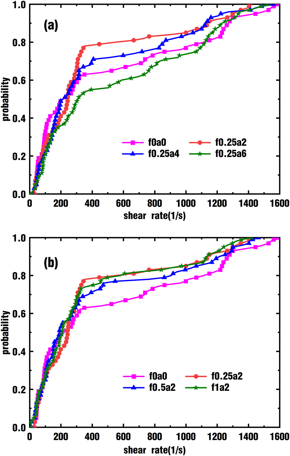
Effect of different excitation types on the cumulative probability distribution of shear rate at t = 8 s: (a) under different amplitudes and (b) under different frequencies.
It can be seen from the diagram that the shear rate is distributed in the interval [0, 1600], and less than 10 % of the particles are subjected to shear rate values greater than 1300 s−1. Figure 8a shows that the corresponding probabilities for shear rate 400 s−1 under four different working states are 0.63, 0.78, 0.7, and 0.55, respectively. That result suggests that compared with the steady state f0a0, the melt is affected by more shear rates with low value under the states f0.25a2 and f0.25a4, while the melt under f0.25a6 is affected by more high-value shear rates. The graph Figure 8b shows that the corresponding probabilities for the shear rate of 400 s−1 under four different working states are 0.63, 0.78, 0.71, and 0.75, respectively. Similarly, compared with f0a0, the melt is affected by more low-value shear rate under other conditions with rotational speed pulsation excitation, which is basically consistent with the analysis in Figure 7.
3.4 Mixing index
In order to characterize the form and intensity of particle motion in melt, mixing index λ is introduced [16, 17], defined as follows:
where
Figure 9 shows the comparison of the curves of the mixing index of the melt under different speed pulsation frequencies and pulsation amplitudes. It can be seen from Figure 9a that the mixing index rapidly increases to the maximum value within 0–2 s. Then, within 2–8 s, the mixing index decreases slowly, and only the f0.25a6 curve moves upward in reverse. For most of the time, the mixing index curves with superposition of pulsating excitation are above the curve without pulsating excitation, and the mixing index increases with the growing of amplitude, indicating that increasing the amplitude can greatly enhance the tensile effect of materials in the flow channel. As can be seen from Figure 9b, the curve trend develops nearly the same with Figure 9a. In the early 0–2 s, the mixing index rises rapidly to the maximum; then, within the following 2–8 s, the mixed index oscillation decreases. With the increase of pulsating frequency, the mixing index is gradually away from the mixing index corresponding to the nonpulsation case, indicating that increasing the pulsating excitation frequency can greatly strengthen the tensile effect of the material in the flow channel. It should be noted that the mixing index under f0.25a2 condition decreases significantly within 7–8 s, which was not conducive to continuously ensure a stable strong tensile flow field. In summary, the superposition of pulsation excitation on rotational speed can form strong shear flow field and tensile flow field and then force the melt material to conduct intense shear flow and tensile flow.

Effect of (a) different vibration amplitudes and (b) different vibration frequencies on the melt mixing index as a function of time.
4 Conclusions
In this paper, a set of speed pulsation drive system for the plasticizing screw is innovatively designed. According to the system, the following results are found by numerical simulation:
Compared with the nonpulsation excitation of screw speed, the superposition of rotational speed pulsation excitation will increase the number of particles retained in the flow channel, making it easy to accumulate materials in the screw and not conducive to material transportation.
The melt pressure in the channel decreases gradually with the increase of pulsation amplitude and pulsation frequency. There is a certain pulsating excitation parameter, which makes it minimum and most stable for the numerical fluctuation of the flow channel melt pressure. The melt in the channel is subjected to lower shear rate under small amplitude conditions and higher shear rate under large amplitude conditions.
Compared with increasing pulsation amplitude, increasing pulsation frequency is more conducive to obtain higher mixing index, which can form strong shear flow field and tensile flow field and then force the melt material to undergo intense shear flow and tensile flow.
Finally, the influence of different pulsation parameters on the mixing process is significantly different. It is of great importance to improve the excitation control of screw speed pulsation and further optimize the method and principle of screw speed fluctuation drive so as to provide theoretical reference for obtaining higher performance plasticizing system and engineering application.
Funding source: National Natural Science Foundation of China
Award Identifier / Grant number: 11972023
Funding source: Special Project of College-enterprise Cooperation of Guangdong Polytechnic of Industry and Commerce
Award Identifier / Grant number: 2021-CJXY-06
Funding source: Scientific Research Innovation Team Project of Guangdong Polytechnic of Industry and Commerce
Award Identifier / Grant number: 2021-TD-03
-
Research ethics: Not applicable.
-
Author contributions: All the authors have accepted responsibility for the entire content of this submitted manuscript and approved submission.
-
Competing interests: The authors declare no conflicts of interest regarding this article.
-
Research funding: The authors wish to acknowledge the financial support from the National Natural Science Foundation of China (no. 11972023), Special Project of College-Enterprise Cooperation of Guangdong Polytechnic of Industry and Commerce (no. 2021-CJXY-06), and Scientific Research Innovation Team Project of Guangdong Polytechnic of Industry and Commerce (no. 2021-TD-03).
-
Data availability: The raw data can be obtained on request from the corresponding author.
References
1. Qu, J. P., Xu, B. P., Jin, G., He, H. Z., Peng, X. F. Performance of filled polymer system under novel dynamic extrusion processing conditions. Plast. Rubber Compos. 2002, 10, 432–435.10.1179/146580102225008330Search in Google Scholar
2. Connelly, R. K., Kokini, J. L. Examination of the mixing ability of single and twin screw mixers using 2D finite element method simulation with particle tracking. J. Food Eng. 2007, 79, 91–94, https://doi.org/10.1016/j.jfoodeng.2006.03.017.Search in Google Scholar
3. Cheng, W. K., Yang, Y., Jiang, S. X., Wang, J. J., Gu, X. P., Feng, L. F. Mixing intensification in a horizontal self-cleaning twin-shaft kneader with a highly viscous Newtonian fluid. Chem. Eng. Sci. 2019, 201, 437–447, https://doi.org/10.1016/j.ces.2019.03.005.Search in Google Scholar
4. Casulli, J., Clermont, J. R., Von Ziegler, A., Mena, B. The oscillating die: a useful concept in polymer extrusion. Polym. Eng. Sci. 1990, 23, 1551–1556, https://doi.org/10.1002/pen.760302310.Search in Google Scholar
5. Jiang, X. J., Huang, M. J., Feng, W. J., Pan, X. B., Wang, X. Y., Li, Q. Study of wave screw for injection molding long glass fiber reinforced polypropylene. Eng. Plast. Appl. 2020, 10, 45–51.Search in Google Scholar
6. Fridman, M. L., Peshkovsky, S. L. Molding of polymers under conditions of vibration effects. Adv. Polym. Sci. 1993, 41–79.10.1007/BFb0025814Search in Google Scholar
7. Wong, C. M., Chen, C. H., Isayev, A. I. Flow of thermoplastics in an annular die under parallel oscillation. Polym. Eng. Sci. 1990, 24, 1574–1584, https://doi.org/10.1002/pen.760302404.Search in Google Scholar
8. Isayev, A. I., Wong, C. M., Zeng, X. Effect of oscillations during extrusion on rheology and mechanical properties of polymers. Adv. Polym. Technol. 1990, 1, 31–45, https://doi.org/10.1002/adv.1990.060100104.Search in Google Scholar
9. Xu, B. P., Liu, B., Liu, Y., Tan, S. Z., Du, Y. X., Liu, C. T. Numerical simulation of distributive mixing under a pair of triangular cams. CIESC J. 2020, 8, 3545–3555.Search in Google Scholar
10. Liu, J., Zhu, X. Chaotic mixing analysis of a novel single–screw extruder with a perturbation baffle by the finite-time Lyapunow exponent method. J. Food Eng. 2019, 3, 287–299, https://doi.org/10.1515/polyeng-2018-0037.Search in Google Scholar
11. Qu, J. P. A method and equipment for the electromagnetic dynamic plasticating extrusion of polymer. E.P. Patent 0444306B1, March 29, 1995.Search in Google Scholar
12. Qu, J. P. Plastics electromagnetic dynamic plasticating extrusion machine (award lecture). In 3rd International Conference on Manufacturing Technology, Hong Kong, December 13–16, 1995.Search in Google Scholar
13. Rathod, M. L., Kokini, J. L. Extension rate distribution and impact on bubble size distribution in Newtonian and non-Newtonian fluid in a twin screw co-rotating mixer. J. Food Eng. 2016, 169, 214–227, https://doi.org/10.1016/j.jfoodeng.2015.09.007.Search in Google Scholar
14. Liu, T. L., Du, Y. X., He, X. Y. Statistical research on the mixing properties of wave screw based on numerical simulation. Int. Polym. Process. 2023, 38, 200–213, https://doi.org/10.1515/ipp-2022-4253.Search in Google Scholar
15. Liu, T. L., He, X. Y., Sun, T. T., Zhao, J. A screw drive system and extruder. C. N. Patent 113199728A, August 3, 2021.Search in Google Scholar
16. Liu, T. L., Du, Y. X. Numerical simulation on the mixing behavior of pin unit under vibrant enhancement. Polym.–Plast. Technol. Eng. 2011, 12, 1231–1238, https://doi.org/10.1080/03602559.2011.574672.Search in Google Scholar
17. Ottino, J. M. The Kinematics of Mixing: Stretching, Chaos and Transport. Cambridge University Press: Cambridge, 1989.Search in Google Scholar
© 2023 Walter de Gruyter GmbH, Berlin/Boston
Articles in the same Issue
- Frontmatter
- Material Properties
- Effect of super critical carbon dioxide and alkali treatment on oxygen barrier properties of thermoplastic starch/poly(vinyl alcohol) films
- Promoting antibacterial activity of polyurethane blend films by regulating surface-enrichment of SiO2 bactericidal agent
- Improving anti-aging performance of terminal blend rubberized bitumen by using graft activated crumb rubber
- An experimental investigation of flame retardancy and thermal stability of treated and untreated kenaf fiber reinforced epoxy composites
- Preparation and properties of ABS/BNNS composites with high thermal conductivity for FDM
- Development of a high-strength carrageenan fiber with a small amount of aluminum ions pre-crosslinked in spinning solution
- Development and characterization of new formulation of biodegradable emulsified film based on polysaccharides blend and microcrystalline wax
- Study on the volatilization behavior of monomer and oligomers in polyamide-6 melt by dynamic film–forming device
- Engineering and Processing
- Numerical simulation on the mixing behavior of double-wave screw under speed sinusoidal pulsating enhancement induced by differential drive
- Numerical and experimental studies on the influence of gas pressure on particle size during gas-assisted extrusion of tubes with embedded antibacterial particles