Prediction of the maximum flow length of a thin injection molded part
-
Sara Liparoti
 ,
Vito Speranza
,
Vito Speranza

Abstract
One of the most significant issues, when thin parts have to be obtained by injection molding (i.e. in micro-injection molding), is the determination of the conditions of pressure, mold temperature, and injection temperature to adopt to completely fill the cavity. Obviously, modern computational methods allow the simulation of the injection molding process for any material and any cavity geometry. However, this simulation requires a complete characterization of the material for what concerns the rheological and thermal parameters, and also a suitable criterion for solidification. These parameters are not always easily reachable. A simple test aimed at obtaining the required parameters is then highly advantageous. The so-called spiral flow test, consisting of measuring the length reached by a polymer in a long cavity under different molding conditions, is a method of this kind. In this work, with reference to an isotactic polypropylene, some spiral flow tests obtained with different mold temperatures and injection pressures are analyzed with a twofold goal: on one side, to obtain from a few simple tests the basic rheological parameters of the material; on the other side, to suggest a method for a quick prediction of the final flow length.
1 Introduction
Micro-injection molding process is widely diffused because of an increasing demand for miniaturized parts that are adopted in many fields, from the electronic to the biomedical sector. It is not easy to determine the conditions that allow the complete filling of the cavity during the micro-injection molding, mainly because the fast cooling occurring during the filling can cause a premature solidification. Thus, there is a need for simplified strategies that allow determining the capability of a melt to advance inside a cavity with at least one micrometrical dimension. The simplified strategies are especially required when incomplete material characterizations, in terms of rheology and thermal properties, are available.
The simulation by commercial software of the injection molding process, usually adopted for the determination of the flow length, involves considerable amount of interactions, costs, and computation time. Additionally, it would be difficult to obtain reliable numerical predictions when the rheology, the thermal properties, and the solidification conditions are not properly known.
During the last decades, several attempts were carried out to predict the flow length, viscosity, and the pressure drop during the injection molding process by simplified strategies. Baumann and Steingiser [1] and Pezzin [2] simulated the filling of the cavity with polycarbonate and polystyrene with the aim of obtaining the viscosity (flow curves) of these polymers. The viscosity values obtained from simulation were very similar to those obtained by experimental rheological tests. Claverìa et al. [3] adopted a spiral flow test to obtain the rheological data of a polypropylene. In the model they adopted, the viscosity dependence on the shear rate and temperature was described by a second-order equation. They applied the aforementioned strategy also to the recycled polymer and obtained results comparable with the experimental rheological data. Osswald and coworkers [4] developed a numerical method to determine the flow length of polystyrene and polypropylene into a spiral cavity. Their predictions were consistent with the experimental observations. Kazmer and coworkers [5] compared the length of the flow injecting into a spiral cavity with that one injected into a quarter of disk cavity. Their conclusion was that spiral flow tends to overpredict polymer flow length. Rao et al. [6] adopted dimensionless parameters to characterize the variations on flow length into a spiral cavity, in several injection conditions. Mercado and coworkers [7] developed a simulation method for the determination of viscosity during spiral flow test in the presence of mold decoration. All these methods and strategies were applied to the conventional injection molding process.
In this work, the micro-injection molding process was carried out with a spiral cavity under several mold temperatures and injection pressures, on an isotactic polypropylene (iPP), which properties (rheological, thermal) are well known. The results are analyzed with a twofold aim: to obtain the basic rheological parameters of the material and to determine a solidification criterion for a quick prediction of the final flow length. In order to confirm the proposed analysis, numerical simulations of performed spiral tests were conducted by a commercial software for the injection molding simulations.
2 Materials and methods
The T30G PP commercial grade (Basell, Ferrara, Italy) was selected for the spiral flow tests. A deep characterization of rheology and crystallization kinetics, in both quiescent and flow conditions, is reported elsewhere [8], [9], [10].
The injection molding machine adopted in this work is an HAAKE Minijet II by Thermo Scientific (Waltham, MA, USA). This machine is a mini-injection molding system that adopts a pneumatic piston to control the pressure during the molding. The molds for HAAKE Minijet II present a truncated cone shape, with a diameter that changes from 50 (at the gate side) to 35 mm over a length of about 90 mm. The cavity, 0.5 mm thick, adopted for the molding tests is sketched in Figure 1.
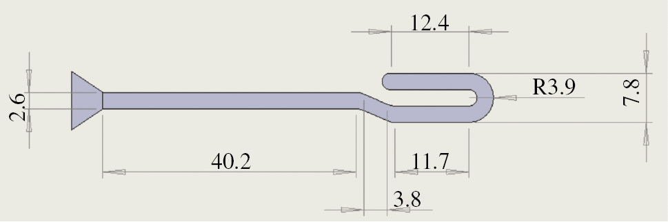
Sketch of the cavity adopted during the spiral flow tests. The dimensions are indicated in millimeters. The cavity thickness is 0.5 mm.
All the tests were performed with an injection temperature of 200°C and with 1 s injection time. Several mold temperatures were selected for the spiral flow tests: 28, 50, 80, 110, 140, and 150°C. The mold was cooled down to 25°C in a water bath after each test. Three injection pressures were selected: 13, 20, and 40 MPa. For each condition, five tests were performed.
The mini injection molding machine was equipped with a transducer position (Gefran mod. PK-M-100, Provaglio di Isea, Brescia, Italy) for the measurement of the piston run. Ten volts was applied by a power supplier (Agilent mod. E3630A, Santa Clara, CA, USA), and the signal was acquired by a dashboard (National Instruments mod. USB-6210, Norton, MA, USA) controlled by a software developed by LabView 2013 SP1 (Norton, MA, USA). The relationship among the measured voltage and the length of the piston path (Lp) is given by Equation 1.
where f.s. is the full scale of the piston, expressed in millimeters, and of the power supplier, expressed in volts. On its turn, the length of the piston path can be related to the flow path length inside the cavity, by the relationship reported in Equation 2:
where Scil and Sc are the section of the piston and the section of the cavity, respectively.
Thin slices (70 μm) were cut from each sample in the flow-thickness plane direction by Leica RM 2265 (Wetzlar, Germany) slit microtome. The slices were observed by Olimpus BX51 (Segrate, Milano, Italy) optical microscope with crossed polarizers. The slices were rotated of 45° with respect to the direction of one of the polarizers.
Infrared (IR) spectroscopy was performed by a Perkin Elmer (Spectrum 100, Milano, Italy) FTIR instrument in the range 4000–4500 cm−1. The orientation of the sample was evaluated by the dichroic ratio and the evaluation of the Herman’s factor. The procedure is reported elsewhere [11].
3 Results
3.1 Spiral flow tests
The results related to the length of each molded sample are summarized in Table 1 for the tests performed with 1 s injection time.
Flow length measured for the spiral flow tests performed under different mold temperatures (Tm) and injection pressures (Pinj).
| Pinj (MPa) | Tm (°C) | ||||
|---|---|---|---|---|---|
| 28 | 50 | 80 | 110 | 140 | |
| 13 | 10.8±0.3 | 11.1±1.2 | 11.8±0.7 | 12.9±1.0 | 18.6±0.2 |
| 20 | 13.0±0.7 | 13.8±0.8 | 14.8±0.4 | 15.9±0.7 | 26.5±1.2 |
| 40 | 16.8±0.5 | 17.3±0.3 | 20.1±0.8 | 25.6±0.5 | 38.2±1.3 |
Figure 2 shows the cavity filling length versus the mold temperature, with three injection pressures, 13, 20, and 40 MPa. Both the mold temperature and the injection pressure influence the cavity filling length.
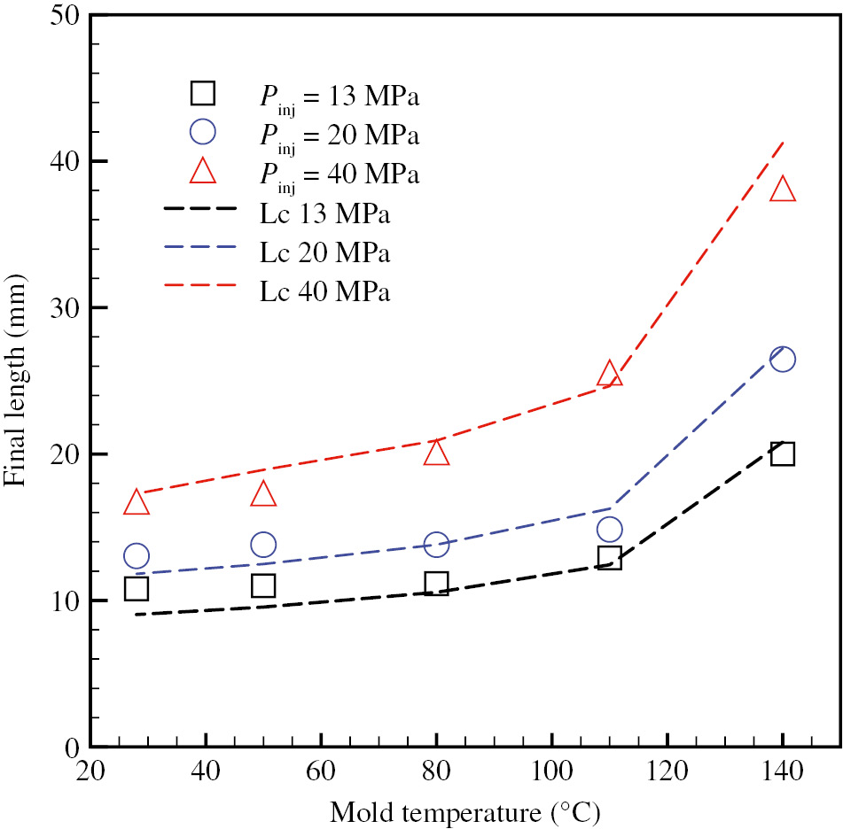
Length measured on the samples produced with different mold temperatures and injection pressures. The dashed lines represent the final length predicted of Equation 23 with h/H=0.38 and β=1.
The mold temperature increase induces an increase of the cavity filling length, obviously due to a later solidification. The increase of the injection pressure also induces an increase of the cavity filling length. For the test conducted with a mold temperature of 150°C and injection pressure of 40 MPa, the cavity resulted to be always completely filled. This gives an indication of the fact that the no-flow condition is reached at a temperature between 140 and 150°C.
Figure 3A shows the optical micrographs of the samples obtained with 140°C mold temperature and different injection pressures at 10 mm from the gate.
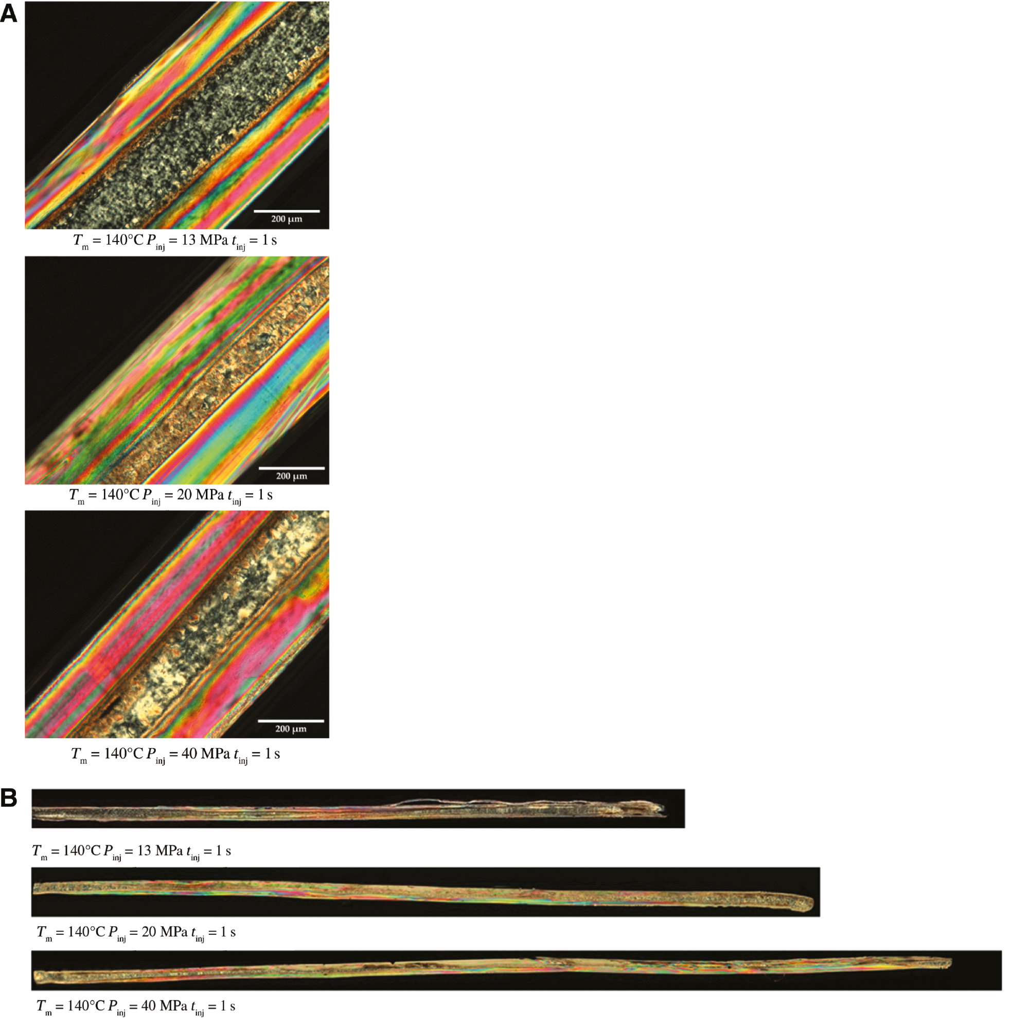
(A) Optical micrographs of the samples obtained with Tm=140°C, tinj=1 s and different injection pressures, taken at 10 mm from the gate position. (B) Optical micrographs of the samples obtained with Tm=140°C, tinj=1 s and different injection pressures, along the whole sample length, from the gate to the tip.
The samples are characterized by a skin core morphology, with the oriented structures (the colored bands in Figure 3A) close to the sample surface and un-oriented structures in the core. The formation of the oriented structures is due to the interplay between the flow field and the solidification: under strong flow and fast cooling, typical of the areas close to the sample surface, the formation of oriented structures can be observed, whereas under weak flow and slow cooling, the polymer chains have enough time to form more isotropic structures, namely the spherulites [12].
Figure 3B shows the optical micrographs of the whole sample obtained with 140°C mold temperature and different injection pressures. Figure 4A shows the distribution of the thickness of the oriented layers along the flow path. Concerning the distribution along the flow path, it is noticed that the oriented structures are mainly located in the central part of the sample. The sample tips are characterized by un-oriented structures, because in that area, the flow is not enough to assure the formation of oriented structures [12]. Close to the gate, the thickness of the layer characterized by oriented structures is smaller with respect to the central part of the samples, as in this area the temperature is closer to the temperature of the piston (200°C as mentioned in the experimental section).

(A) Thickness of the oriented layers versus the flow path length, evaluated for the samples obtained with Tm=140°C, tinj=1 s and different injection pressures. (B, C) Herman’s factor versus the flow path length, evaluated for the samples obtained with Tm=140°C, tinj=1 s and different injection pressures. (B) Analysis of the peak λ=1256 cm−1. (C) Analysis of the peak λ=1220 cm−1.
The samples obtained with Pinj=13 MPa and Pinj=20 MPa show the highest values of the thickness of the oriented layers at about 10 mm distance from the gate. The sample obtained with Pinj=40 MPa shows the highest values of the thickness of the oriented layers after a distance of about 17 mm from the gate.
The orientation distribution inside the samples was measured from the FTIR spectra, which allow the determination of the Herman’s factor. This factor varies between −0.5 and 1.0, with −0.5 representing the perpendicular orientation with respect to the direction of the flow. For the case of parallel orientation with respect to the flow, Herman’s factor ranges from 0 to 1, with 0 corresponding to random orientation and 1 to the perfect alignment with respect to the flow direction (the reference axis). The oriented structures, in the injection molding process, correspond to fibrils, crystals that mainly grow along the flow direction, with limited growth in the direction perpendicular to the flow [13]. Figure 4B and C show the distribution of the Herman’s factor along the flow path. Two peaks of the FTIR spectra were analyzed, at a wave number (λ) of 1256 and 1220 cm−1, the first one related to the crystalline phase, the second one related to the amorphous part.
Figure 4 shows that excluding the region very close to the gate, the orientation decreases from the gate, where the Herman’s factor is close to 1, for the samples obtained with an injection pressure of 20 and 40 MPa, to the tip, where the Herman’s factor decreases down to 0.2. The highest orientation was measured at the same distance from the gate characterized by the highest thickness of the oriented layer (see Figure 3). The sample obtained with an injection pressure of 1 MPa shows smaller values of the Herman’s factor, mainly due to the decrease of the flow intensity at lower injection pressures.
Indeed, orientation can be easily related to the flow intensity: the shorter the distance from the gate, the higher the flow intensity, the higher the orientation [14]. Very close to the gate, because of the high temperature, the relaxation time is short and thus the orientation can be low. Far from the gate, the flow becomes less intense, because of the pressure decrease along the flow path; thus, the polymer chains can crystallize in almost quiescent condition. As a result, close to the tip, poorly oriented structures and spherulites can be observed.
3.2 Estimation of polymer rheology from the time evolution of flow length
All the samples produced in this work were obtained without holding stage; this means that the shrinkage due to the material solidification and crystallization was not compensated. This procedure allows analyzing the effect of the injection pressure on the flow length with the aim of modelling the filling process. The filling of the material into the cavity was analyzed by recording the piston path and correlating this movement to the flow length inside the cavity (Equation 2), as mentioned in the experimental section. Because during the experiments the machine performs a control of the injection pressure, the flow rate changes to keep constant the injection pressure during the experiment, and thus, the flow can be considered as a pressure-driven flow. Figure 5A shows the flow length (Lsper) inside the cavity recorded during the experiments performed with Tm=140°C, tinj=1 s, and different injection pressures.
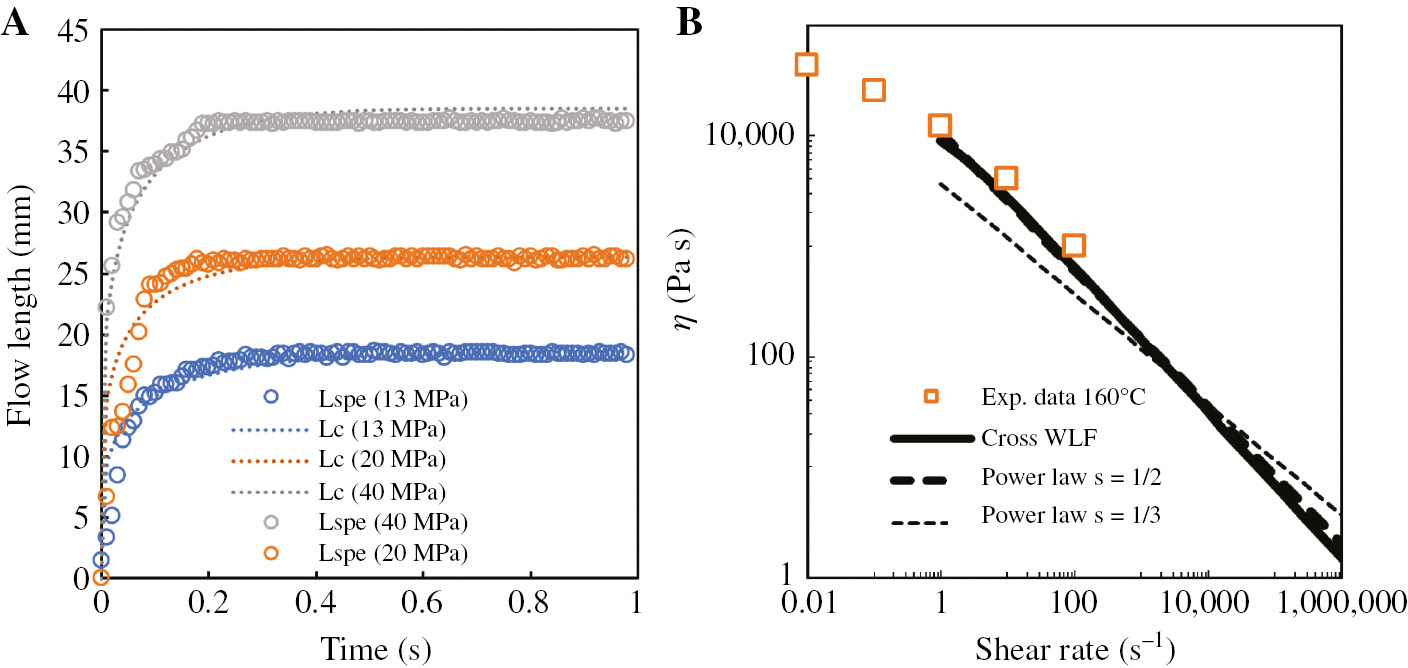
(A) Flow length recorded during the experiments performed with Tm=140°C and tinj=1s, with different injection pressures. The full lines represent the predicted evolution of the flow length, Lc, with s=1/2. (B) Comparison between the viscosity values predicted by the power-law based models proposed in this paper, the viscosity experimental data at 160°C, and the values of the viscosity evaluated by Cross-WLF at zero pressure.
The flow length, as expected, increases with the injection pressure.
In order to determine the rheology of a polymer from the spiral flow tests, one has to model the history of the length at a certain injection pressure. For a polymer melt filling, a rectangular cavity, having a width W and a thickness H, the relationship among the stress, τxy, gradient along the thickness (y) and the pressure drop along the cavity length (x) is given by Equation 3.
The integration along the thickness y gives
with τxy=0 for y=0 (namely at the midplane).
Under the hypothesis of a viscous fluid and viscosity described by a power law, the stress is given by Equation 5:
where η0 is the consistency index, n is the flow behavior index, and vx is the velocity along the flow direction (x). Thus, for y >0,
On integrating and using the no-slip boundary condition (y=H; vx=0), it is possible to obtain the velocity profile along the cavity thickness (y) as a function of the pressure drop (in the following, the reciprocal of the flow index will be adopted: m=1/n):
It is possible to evaluate the flow rate Q by the Equation (8):
During any increment of time dt, the fluid volume injected into the channel is [15], [16]
Assuming a pressure profile linearly decreasing with x and indicating with P the difference between the injection pressure Pinj and the pressure at the tip, it is possible to relate the flow length, L(t), to the pressure drop:
In the model considered in this work, sketched in Figure 6, the polymer flows with a constant temperature inside the central part of the cavity. The section through which the melt fills the cavity reduces during the process, as the formation of a frozen layer close to the cavity surface takes place. The temperature at the interface between melt and solid, located at a distance δ from the mold walls, is equal to the so-called no-flow temperature, Tf. The section available to the flow will be indicated as h(t).
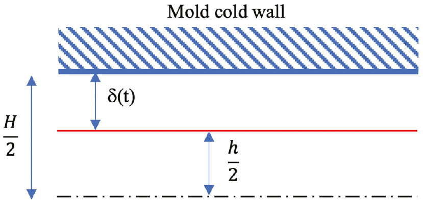
Sketch of the cavity thickness decrease due to the formation of the frozen layer.
Thus, Equation (11) has to be rewritten with h(t) instead of H.
Barrie [17] proposed the following relationship to describe the formation of the frozen layer during the cavity filling, also applied by other authors [18]:
C and s are constants and Barrie found that s=1/3 for many polymers. At the solidification time tf, δ=H/2, thus, it is possible to calculate the value of the constant C.
Therefore, it is possible to obtain h(t):
Substituting Equation 15 in Equation 12 and integrating, the melt advancement with time can be obtained as follows:
Equation 16 provides a relationship between time during which the melt fills the cavity and the flow path length in the spiral-shaped rectangular section cavity. When t=tf, the equation gives the final value of the final length of the sample.
Some authors adopt an exponent s=1/2 in Equation 13 [19], in this case the melt advancement can be obtained as follows:
Again, when t=tf, the equation gives the final value of the length of the sample.
The relationships given by Equations 16 and 18 allow evaluating the rheological parameters of a resin comparing the predicted flow path lengths with the experimental ones shown in Figure 5. In particular, it is possible to obtain values of η0 and tf, for selected values of 1/m. It has to be pointed out that the values of the solidification time tf evaluated from Equations 16 and 18 are close to 1 s for all the considered values of 1/m.Table 2 summarizes the results of η0 and 1/m.
Rheological parameters n and η0, evaluated by equation 17 (with s=1/3) as function of the injection pressure, Lf and tf.
| s | 1/m | Deviation | η0 (Pan s) | η0 (Pan s) | η0 (Pan s) |
|---|---|---|---|---|---|
| Pinj=13 MPa | Pinj=20 MPa | Pinj=40 MPa | |||
| 1/3 | 0.10 | 34.00 | 51,029 | 76,834 | 106,963 |
| 0.20 | 27.81 | 25,160 | 35,582 | 47,855 | |
| 0.30 | 20.93 | 13,043 | 17,420 | 22,618 | |
| 0.34 | 18.70 | 10,098 | 13,118 | 16,909 | |
| 0.35 | 18.28 | 9475 | 12,243 | 15,727 | |
| 0.40 | 17.07 | 6890 | 8690 | 10,937 | |
| 0.50 | 16.99 | 3669 | 4406 | 5361 | |
| 0.60 | 18.08 | 1965 | 2243 | 2643 | |
| 0.70 | 22.45 | 1051 | 1146 | 1304 | |
| 1/2 | 0.10 | 32.35 | 59,528 | 89,630 | 124,772 |
| 0.20 | 24.46 | 31,315 | 44,326 | 59,417 | |
| 0.30 | 18.49 | 16,900 | 22,958 | 29,363 | |
| 0.34 | 17.03 | 13,331 | 17,447 | 22,408 | |
| 0.35 | 16.93 | 12,551 | 16,351 | 20,915 | |
| 0.38 | 16.87 | 10,480 | 13,468 | 16,924 | |
| 0.40 | 16.89 | 9298 | 11,829 | 14,877 | |
| 0.50 | 18.01 | 5133 | 6215 | 7567 | |
| 0.60 | 19.96 | 2831 | 3274 | 3852 | |
| Cross-WLF at | 0.37 | 10,009 | 10,474 | 11,887 | |
| 0.37 | 10,869 | 11,608 | 13,193 |
The values of η0 given by WLF are also reported.
Table 2 shows also the values of the deviation, evaluated as sum of the absolute values of the differences among the experimental flow length and the calculated ones at each time. The values of η0 depend on the injection pressure: the higher the injection pressure is, the higher the values of η0. This result is consistent with the fact that the pressure increase induces an increase of the viscosity [20], [21], [22]. Is it possible to compare the values of the η0 found applying the aforementioned models to the values estimated adopting the model reported in the literature to describe the rheological behavior of the iPP adopted in this work. The model proposed in the literature is a Cross-Williams-Landel-Ferry (Cross-WLF) equation, which takes also into account the effect of pressure on viscosity [9]. For the temperature, pressure, and shear rate ranges considered in this work, the parameters of Cross-WLF are reported in the literature [23]. In particular, the Cross-WLF model for high shear rate can be approximated by a power law having the same exponent (1/m) of Cross-WLF and the consistency index equal to the Cross-WLF viscosity evaluated with a shear rate equal to 1 s−1; these values are reported in Table 2. Both the rheological data, those obtained from Cross-WLF and the experimental ones, are referred to temperatures of 160 and 170°C, namely, intermediate values between the injection temperature and the mold temperature. In order to consider the effect of pressure, the rheological data are calculated at the arithmetic average between the maximum pressure (equal to Pinj) and the minimum pressure (equal to zero), namely, at Pinj/2.
The minimum values of the deviation were obtained with 1/m=0.50, for s =1/3, and 1/m=0.38, for s=1/2. Figure 5B shows the comparison among the viscosity values predicted by the power law models (adopting the values of 1/m and η0, which correspond to the minimum value of the deviation), the viscosity experimental data at 160°C, and the values of the viscosity evaluated by Cross-WLF. The comparison shown in Figure 5B confirms that the values of the viscosity are reasonably well predicted from Equation 18, with s=1/2. Additionally, the Cross-WLF model and the power law model with s=1/2 proposed in this paper show very close values and both correctly predict the experimental data at 160°C. The shear rate characteristic of the tests ranges from 300 to 5000 s−1; this confirm the reliability of the power law model proposed in this paper in the description of the viscosity behavior.
Figure 5B shows the comparison among experimental and calculated flow path lengths obtained selecting the values of η0 and 1/m that give the minimum deviation for s=1/2 (Equation 18).
The behavior of L(t) is reasonably well described by the model reported in this paper; this is a further confirmation that the flow behavior is correctly predicted by the model with s=1/2.
3.3 Prediction of maximum flow length
When the rheology of the material (namely, 1/m and η0) are known, Equations 17 and 19 allow the determination of the flow length, which can be reached during an injection molding test. The only unknown becomes the solidification time, tf, whose determination requires the solution of the thermal problem. Several analysis have been proposed in the literature for the determination of the solidification time into a long rectangular cavity (e.g. by Wissbrun [24] or Richardson [25]). The phenomena to be taken into account are axial convection, transverse conduction, and viscous dissipation. The former two are kept into account by the Graetz number, the latter by the Brinkman number.
For the cases under analysis in this work, the Graetz and Brinkman numbers can be expressed as follows:
α is the thermal diffusivity, Tf is the temperature at the boundary of the frozen layer, namely the no-flow temperature. As mentioned above, Tf was estimated in the range from 140 to 150°C. In the following, we will assume Tf=147°C.
Both Gz and Br depend on time through the value of h. It is easy to find that
is independent on time.
Being, in our experiments, P of the order of 107 Pa, α of 10−7 m2/s, k of 10−1 W/mK, (Tinj–Tf) of 102 K, and m of 100, the order of magnitude of
A solidification criterion can be determined by considering a macroscopic energy balance in the cavity and comparing the convective heat entering the cavity, Econv, with the conductive heat lost toward the cavity surface, Econd.
The order of magnitude of the former can be evaluated as
and the order of magnitude of the latter as
where
When Econv is larger than Econd, it can be assumed that solidification cannot take place (and indeed h remains close to H). As soon as Econd overcomes Econv, h decreases quickly, and solidification happens. Considering Equations 23 and 24, the ratio between the two heat quantities is
in which
Solidification takes place when the Econd and Econv become comparable, namely when
β being a constant (of order of magnitude 1).
On this basis, the value of the final flow length is immediately drawn from Equation 20.
To validate the results and hypotheses of the method proposed in this work, numerical simulations of the injection molding tests were performed by a commercial software. Numerical results and comparisons between predictions and experimental results are reported in Appendix 1, Figures 9–12.
By adopting Equation 28, a description of the final length reported in Figure 2 can be obtained by selecting a suitable value of β and of h/H at solidification. If β is taken as 1, then only the value of h/H at solidification has to be chosen. In Figure 2, the predictions (dashed lines) of the flow lengths are obtained by adopting the values of 1/m and η0 obtained by WLF at 160°C (last line of Table 2) and h/H=0.62. The description is satisfactory, with a value of h/H absolutely reasonable. Obviously, a different value would be found with a different value of β. For instance, for β=0.1, the optimal value of h/H would be 0.34.
It can be observed that the dependence of Lf upon P as provided by Equation 28 is the same resulting from Equations 17 and 19, so that it can be written as follows:
Equation 28 outlines the dependence of the dimensionless time at solidification
where ε is a constant.
The values of tf calculated by Equation 30 for the tests carried out in this work are reported in Figure 7; the values of β and
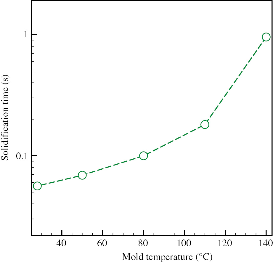
Estimated solidification times for the tests carried out in this work. Tinj=200°C, Tf=147°C.
Figure 7 shows that the solidification time tf at 140°C is close to 1 s. This validates the results reported in Table 2.
3.4 The oriented layer
As indicated in the literature, specifically for this material, the fibrils forms when the amount of work overcomes a critical value, wc, which is of the order of 10 MPa [23].
For the model adopted in this work, which assumes the flow of a power-law fluid in a rectangular cavity, the rate of specific work, given by the product between stress and shear rate, can be expressed as
where y is the distance from the mold wall.
If L(t) is taken from Equation 18, then the amount of work at each specific location y at the end of the process can be written as
where
and b is equal to t/tf.
Assuming that the fibrillar layer forms when w=wc, considering that the work decreases on increasing the distance from the mold wall, then the thickness of the oriented layer can be determined as
Assuming that wc=10 MPa [23], the fraction of oriented layer reported in Figure 8 is obtained. It can be noticed that in the range of pressure adopted in this work, the fraction is weakly dependent on pressure, as also described by the experimental data reported in Figure 3. The maximum fraction of the oriented layer is underestimated by the model by about 15–20% (0.63 instead of 0.75 at 13 MPa, 0.67 instead of 0.8 at 20 MPa, and 0.73 instead of 0.9 at 40 MPa). However, also considering the simplicity of the model, the predicted values can be surely considered good.
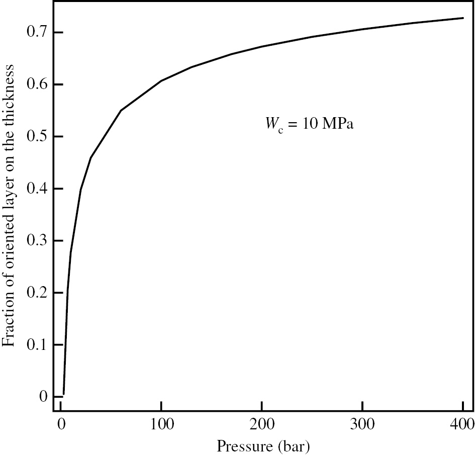
Fraction of oriented layer obtained from Equation 34 for different injection pressure.
4 Conclusions
In this work, the evolution of the cavity filling length with different injection pressures and mold temperatures was measured during spiral flow tests in a thin cavity. As expected, the reached length was found to increase with both the injection pressure and the mold temperature. The tests also allowed to determine the no-flow temperature of the material, in the range 140–150°C. A simple model was adopted and validated to describe the flow advancement during the filling. In this model, the cavity filling length depends only on the pressure difference between the gate (namely the injection pressure) and the tip and the solidification time. The comparison between the experimentally measured evolution of flow-length with time and the predictions of the model allowed a quick estimate of the basic rheological parameters of the material. These parameters where found almost accurate, as demonstrated by comparison with experimental data and the Cross-WLF model used in the literature to describe the rheology of the material adopted in this work.
A simple criterion was also developed to find the solidification time on the basis of a macroscopic energy balance in the cavity. The solidification occurs when the convective heat entering the cavity becomes comparable with the conductive heat lost toward the cavity surface. This allows to evaluate the solidification time from the data of the final filling length. Numerical simulations conducted with the commercial software Moldex3D for the injection molding process validate the hypothesis adopted in the criterion of negligible contribute of the viscous dissipation in the cavity energy balance.
The amount of the fibrillar layer along the sample thickness was evaluated by applying a previously introduced criterion based on the achievement of the critical value of the mechanical work. The values of the thickness of the fibrillar layer were found close to the experimental ones.
Appendix 1: Numerical simulation
Numerical simulations of the spiral flow tests were conducted by adopting Moldex3D version R17 from CoreTech System Ltd (Chupei City, Taiwan). Material database of T30G polypropylene (iPP) (adopted in this work) was created according to its characterization reported elsewhere [11]. All tests considered in this work were simulated in order to confirm the results and hypotheses of the proposed method.
The prediction of the position of melt front for the test performed with 150°C mold temperature and 40 MPa injection pressure is reported in Figure 9; consistently to the corresponding experimental test, at the end of filling time (namely EOF), the polymer completely fills the cavity adopted during the spiral flow tests.
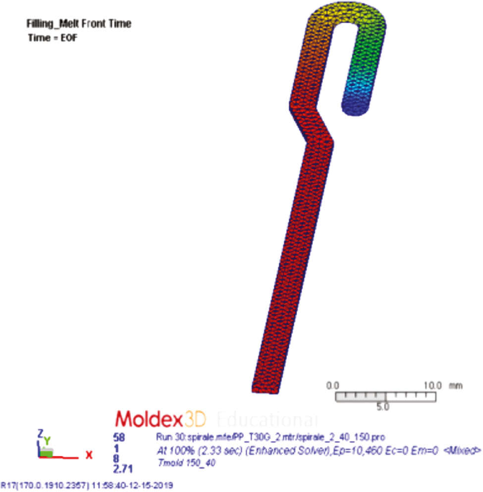
Melt front time predicted with Moldex3D R17 for the experiments performed with Tm=150°C and Pinj=40 MPa.
When smaller mold temperature or injection pressure are adopted, the predicted filling is not complete. Temperature distributions along the sample thickness during the cavity filling at two distances downstream the injection point, 10 and 20 mm, are shown in Figure 10.
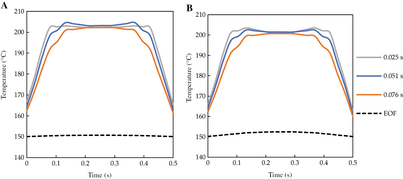
Temperature distribution along the sample thickness predicted with Moldex3D R17 for the experiments performed with Tm=150°C and Pinj=40 MPa at 10 mm (A) and 20 mm (B) downstream the injection point.
In both considered positions, a small increase of temperature (smaller than 3°C) with respect to the injection temperature of 200°C can be detected only in the early stage of the filling. Therefore, the assumption mentioned in this paper to consider negligible the viscous dissipation during the spiral flow tests is verified.
Predictions of the flow lengths evolutions obtained by adopting the proposed model (dashed lines) and Moldex3D simulations (solid lines) are showed in Figure 11 for the tests performed with Tm=140°C and tinj=1 s, with different injection pressures. Predictions obtained with the model proposed in this work are represented as dashed lines, whereas predictions obtained with Moldex3D simulations are represented as solid lines.
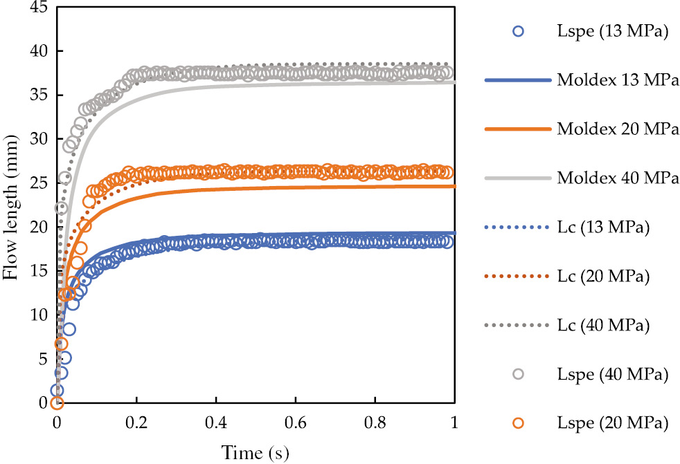
Flow length evolutions obtained from the experiments (see Table 1) and from predictions obtained adopting the model proposed in this paper (Lc) and by Moldex3D. The predictions obtained adopting the model proposed in this paper are represented as dashed lines, the predictions obtained by Moldex3D simulations are represented as solid lines.
Predictions correctly describe the flow length evolutions in all the reported tests even if a better description is achieved with the model proposed in this work. Predictions obtained with Moldex3D slightly underestimate the flow length evolution at higher injection pressures. The predicted solidification time is about 0.7 s, in agreement with what is predicted by the simplified method proposed in this work.
Final lengths for all the tests reported in Table 1 compared with the predicted ones are also reported in Figure 12, where predictions obtained with the model proposed in this work are represented as dashed lines whereas predictions obtained with Moldex3D simulations are represented as solid lines. Moldex3D simulations correctly describe the effect of injection pressure and mold temperature on the final length reached during the tests; predicted final lengths overestimate the measured ones except in the tests performed with mold temperature of 140°C.
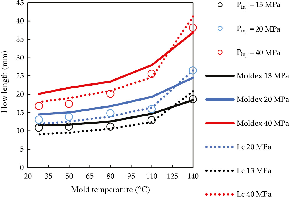
Comparison between the predictions obtained with the model proposed in this work, those obtained by Moldex3D and experimental flow lengths obtained at different mold temperatures and injection pressures. The predictions obtained adopting the model proposed in this paper are represented as dashed lines, the predictions obtained by Moldex3D simulations are represented as solid lines.
Acknowledgements
The authors would to like thank CoreTech System Co. for providing the license of Moldex3D version R17 Professional package.
Conflict of interest statement: The authors declare no conflicts of interest.
References
[1] Baumann GF, Steingiser S. J. Polym. Sci. 1963, 1, 3395–3406.10.1002/pol.1963.100011111Search in Google Scholar
[2] Pezzin G. Polym. Eng. Sci. 1963, 3, 260–269.10.1002/pen.760030405Search in Google Scholar
[3] Clavería I, Javierre C, Ponz L. J. Mater. Process. Technol. 2005, 162–163, 477–483.10.1016/j.jmatprotec.2005.02.065Search in Google Scholar
[4] Buchmann M, Theriault R, Osswald TA. Polym. Eng. Sci. 1997, 37, 667–671.10.1002/pen.11710Search in Google Scholar
[5] Fox CW, Poslinski AJ, Kazmer DO. In Annual Technical Conference – ANTEC, Conference Proceedings; 1998.Search in Google Scholar
[6] Rao NS, Schumacher G, Ma CT. J. Injection Molding Technol. 2000, 4, 92–96.Search in Google Scholar
[7] Martinez A, Castany J, Mercado D. Measurement 2011, 44, 1806–1818.10.1016/j.measurement.2011.09.011Search in Google Scholar
[8] Pantani R, Nappo V, De Santis F, Titomanlio G. Macromol. Mater. Eng. 2014, 299, 1465–1473.10.1002/mame.201400131Search in Google Scholar
[9] Pantani R, Speranza V, Titomanlio G. J. Rheol. 2015, 59, 377–390.10.1122/1.4906121Search in Google Scholar
[10] De Santis F, Pantani R, Titomanlio G. Polymer 2016, 90, 102–110.10.1016/j.polymer.2016.02.059Search in Google Scholar
[11] Pantani R, Coccorullo I, Speranza V, Titomanlio G. Prog. Polym. Sci. 2005, 30, 1185–1222.10.1016/j.progpolymsci.2005.09.001Search in Google Scholar
[12] Speranza V, Liparoti S, Pantani R, Titomanlio G. Materials 2019, 12, 424.10.3390/ma12030424Search in Google Scholar PubMed PubMed Central
[13] Liparoti S, Sorrentino A, Speranza V, Titomanlio G. Eur. Polym. J. 2017, 90, 79–91.10.1016/j.eurpolymj.2017.03.010Search in Google Scholar
[14] Liparoti S, Titomanlio G, Sorrentino A. AIChE J. 2016, 62, 2699–2712.10.1002/aic.15241Search in Google Scholar
[15] Crawford RJ. In Plastics Engineering. Oxford: Butterworth-Heinemann, 1998.Search in Google Scholar
[16] Hsiung CM, Cakmak M. Polym. Eng. Sci. 1991, 31, 1372–1385.10.1002/pen.760311903Search in Google Scholar
[17] Barrie I. Plast. Polym. 1970, 38, 47.10.1016/0031-8914(70)90097-2Search in Google Scholar
[18] White JL, Dietz W. Polym. Eng. Sci. 1979, 19, 1081–1091.10.1002/pen.760191504Search in Google Scholar
[19] Dietz W, White JL, Clark ES. Polym. Eng. Sci. 1978, 18, 273–281.10.1002/pen.760180407Search in Google Scholar
[20] Laun HM. Rheol. Acta 2003, 42, 295–308.10.1007/s00397-002-0291-6Search in Google Scholar
[21] Pantani R, Speranza V, Titomanlio G. Eur. Polym. J. 2017, 97, 220–229.10.1016/j.eurpolymj.2017.10.012Search in Google Scholar
[22] Utracki LA, Sedlacek T. Rheol. Acta 2007, 46, 479–494.10.1007/s00397-006-0133-zSearch in Google Scholar
[23] Liparoti S, Speranza V, Pantani R, Titomanlio G. Materials 2019, 12, 505.10.3390/ma12030505Search in Google Scholar PubMed PubMed Central
[24] Wissbrun KF. Polym. Eng. Sci. 1991, 31, 1130–1136.10.1002/pen.760311510Search in Google Scholar
[25] Richardson SM. Rheol. Acta 1985, 24, 509–518.10.1007/BF01462498Search in Google Scholar
©2020 Walter de Gruyter GmbH, Berlin/Boston
Articles in the same Issue
- Frontmatter
- Editorial
- Special issue: Polymer engineering rheology
- Material properties
- Volume fraction and width of ribbon-like crystallites control the rubbery modulus of segmented block copolymers
- Influence of trisilanol isooctyl POSS content on the structure, morphology and rheological properties of thermoplastic polyurethane (TPU)
- Engineering and processing
- Oscillating shear capillary rheometry (OSCAR) for polymer melts
- Plastic drawing response in the biaxially oriented polypropylene (BOPP) process: polymer structure and film casting effects
- A quantitative study on using digital photoelasticity for characterising the effect of the stretching speed on the necking phenomenon
- Effects of structure and processing on the surface roughness of extruded co-continuous poly(ethylene) oxide/ethylene-vinyl acetate blends
- Processability predictions for mechanically recycled blends of linear polymers
- Prediction of the maximum flow length of a thin injection molded part