Viscous Dissipation and Thermal Radiation effects in MHD flow of Jeffrey Nanofluid through Impermeable Surface with Heat Generation/Absorption
-
Kalpna Sharma


Abstract
This paper investigates steady two dimensional flow of an incompressible magnetohydrodynamic (MHD) boundary layer flow and heat transfer of nanofluid over an impermeable surface in presence of thermal radiation and viscous dissipation. By using similarity transformation, the arising governing equations of momentum, energy and nanoparticle concentration are transformed into coupled nonlinear ordinary differential equations, which are than solved by homotopy analysis method (HAM). The effect of different physical parameters, namely, Prandtl number Pr, Eckert number Ec, Magnetic parameter M, Brownian motion parameter Nb, Thermophoresis parameter Nt, Lewis parameter Le and Radiation parameter Rd on the velocity, temperature and concentration profiles along with the Nusselt number and skin friction coefficient are discussed graphically and in tabular form in details. The present results are also compared with existing limiting solutions.
1 Introduction
Nanotechnology plays an important role in many electronic devices, vehicles, space craft, defense, biomedical science, solar water heating and cooling applications, etc. Choi [1] was the first who employed that if nanometer sized particles are suspended in base-fluid enhanced the heat transfer rate. It was expected that the nanofluids have a better thermal conductivity efficiency than the base fluid like water, ethylene glycol mixture etc. The feature study of nanofluid was originated in the book by Das et al. [2]. Wang and Majumdar [3], Yang et al. [4] and Jahani et al. [5] have done the first theoretical and experimental study on nanofluids with application in science and engineering. Recently Cai et al. [6] developed fractal based approaches to nanofluid and nanoparticle migration. Sheikholeslami and Shehzad [7] studied the convective MHD flow of nanofluid enclosed by heat flux boundary conditions in a porous medium. Hayat et al. [8] investigated the MHD flow of nanofluid due to rotating disk with slip effect. They also studied the heat generation/absorption effects in Oldroyd-B nanofluid induced by a stretching sheet [9]. Hashmi et al. [10] discussed the effects of magnetic field in mixed convective Oldroyd-B nanofluid induced by two infinite isothermal stretching disks. Anwar et al. [11] showed the MHD stagnation point flow of Micropolar nanofluid towards a stretching sheet. There is one important non-Newtonian fluids known as Jeffrey fluid [12– 17] which has been fascinated much by the researchers because of its simplicity. This fluid model is capable of describing the characteristics of relaxation and retardation times.
The investigation of flow of a viscous incompressible fluid over a stretching sheet has been taken up by many researchers because of various industrial applications, such as in the manufacturing of polymer sheets, filaments, and wires. During the manufacturing process, the moving sheet is assumed to stretch on its own plane, and the stretched surface interacts with the ambient fluid both mechanically and thermally. Stretching and shrinking can occur in a variety of materials. Two dimensional flows over a stretching sheet was first studied by Crane [18]. Sakiadas [19] studied the behavior of boundary layer flow due to a moving flat surface immersed in an otherwise quiescent fluid. Bataller [20] studied the effects of thermal radiation on the laminar boundary layer about a flat plate. A variety of aspects of flow and heat transfer of viscous fluid over a flat surface were investigated by many researchers [21–31].
The purpose of this paper is to discuss the analytical solution of the two dimensional MHD flow of viscoelastic Jeffrey fluid through impermeable surface in presence of thermal radiation and viscous dissipation with heat generation / absorption. Similarity transformation has been used to simplify the governing equations, and the reduced boundary value problems are solved analytically by homotopy analysis method (HAM). The HAM has been successfully applied to solve many nonlinear problems in science and engineering [32– 46] because this technique does not depend upon the auxiliary parameter and converges very rapidly the approximate solution into exact one. The main advantage is that HAM is independent of any small/large physical parameters. Unlike all other analytic techniques, the HAM provides us a convenient way to guarantee the convergence of solution series so that it is valid for highly nonlinear problems. The HAM can be applied to solve many nonlinear problems in science, finance and engineering, especially those without small/large physical parameters. So it is conclude that it can be applied directly to nonlinear differential equations without requiring linearization, discretization and therefore, it is not affected by errors associated to discretization. Same as the HAM, the Differential Transform Method (DTM) can overcome the forgoing restriction, assumptions and limitations of traditional perturbation method [47–50]. Recently many researchers and scientists applied the HAM to various fluid flow problems with different geometries. In the last obtained results are compared with those results which are presented by Khan and Pop [51], Wang [52], Gorla and Sidawi [53] and Ramesh et al. [54].
2 Mathematical formulation
Consider a two dimensional flow of an incompressible, electrically conducting viscoelastic Jeffrey fluid model persist the nanoparticle having uniform shape and size over an stretching impermeable sheet. The sheet is coinciding with the plane y = 0 and origin is located at y = 0, by which the sheet is stretching. A constant magnetic field of strength B0 is applied in a direction normal to the plane at y = 0 as shown in the Figure 1. The simplified two dimensional boundary layer equations governing the flow, heat transfer and nano-particle concentration are given by
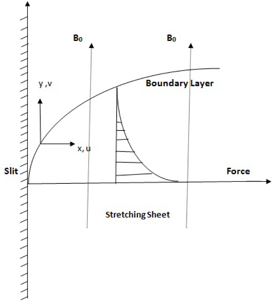
Schematic Diagram of Flow.
The associated boundary conditions are
where u and v are the velocity components in x and y direction, respectively. a > 0 is known as stretching rate, ν is the kinematic viscosity, λ is the ratio of relaxation to retardation times, λ1 is the relaxation time, ρf is the density of base fluid, α is the thermal diffusivity, σ is the electrical conductivity, ρp is the density of the nanoparticles and T is the ambient fluid temperature,
Using Rosseland approximation for radiation, we have
where σ is the Stefan-Boltzman constant, and k* is the mean absorption coefficient. Expanding T4 in terms of Taylor series about T∞ and neglecting higher order terms, we have
By employing the Rosseland approximation of Eq. (8), Eq. (3) takes the form
Introducing the following similarity transformation
where the stream function ψ is defined as
Using equations (10) and (11) in equations (1) to (3), the equations of linear momentum, energy and concentration with their corresponding boundary conditions are reduced as follows
subject to the boundary conditions are as follows
where
The skin friction coefficient, the local Nusselt number and Sherwood number are defined as
where τw is the shear stress along the stretching surface, qw is the surface heat flux and qm is the mass flux, are given by
respectively.
Using the non-dimensional variables in equation (16), we get
where
3 Homotopy analysis method
The homotopy analysis method was derived from the fundamental concept of topology known as homotopy. The basic ideas of the homotopy analysis method (HAM) are here presented by considering the following nonlinear differential equation
where A is a nonlinear differential operator, u(η) is the unknown solution of the equation (19) and η is an independent variable. For simplicity, we ignore all boundary or initial conditions, which can be treated in a similar way. Applying the HAM to solve equation (19), one can construct the so called zeroth order deformation equation, as follows
Where p ∊ [0, 1] is an embedding parameter, ℏ ≠ 0 is an auxiliary parameter, L is a properly selected auxiliary linear operator satisfying L(f) = 0 when f = 0.H(η) ≠ 0 is an auxiliary function and u0 (η) is an initial guess of u(η). Further, it is assumed that at p = 0, the function û(η; p) has derivatives up to infinity. Thus the variation of p from 0 to 1 is the continuous variation of û(η; p) from initial guess u0 (η) to the unknown function u(η) of equation (19). In topology, this type of variation is called deformation, where u0 (η) and u(η) are called homotopic.
Expanding û(η; p) in Taylor series with respect to embedding parameter p, we obtain
where
The convergence of the series (20) depends upon the auxiliary parameter ℏ. If it is convergent at p = 1, one has
which one of the solutions of the original nonlinear equation, as proven by Liao [32–34]. Define the vectors
Differentiating the zeroth-order deformation equation (20)m-times with respect to p and then dividing them by m! and finally setting p = 0, we get the following mth-order deformation equation:
where
and
It should be highlighted that um (x, t) form ≥ 1 is governed by the linear equation (26) with linear boundary conditions that comes from the original problem, which can be easily solved by the symbolic computation software such as Maple, Mathematica and Matlab.
4 Solution of the problem by the homotopy analysis method
Now for solving the present boundary value problems given by the equations (12) to (14) subject to the corresponding boundary conditions (15) by the homotopy analysis method (HAM) by the rule of solution expression, we express the following initial guess f0, θ0, and φ0 of f(η), θ (η) and φ (η) as follows
and with the auxiliary linear operator as
with the property that
and
where Ci(i = 1..7) are arbitrary constants and are determined by the boundary conditions.
Zeroth order deformation problem
with the boundary conditions as
where p ∊ [0,1] indicates the embedding parameter, ℏf, ℏθ and ℏφ are the nonzero auxiliary parameters and Hf (η), Hθ (η) and Hφ (η) are the nonzero auxiliary functions defined on the rule of solution expressions (exponential, polynomials, algebraic etc.). Here the auxiliary function according to the base function is Hf (η) = Hθ (η) = Hφ (η) = e−η. Moreover the nonlinear operators Nf, Nθ and Nφ are prescribed as
Higher order deformation problem
The mth order deformation equations are as follows:
where
with the boundary conditions
where
For p = 0 and p = 1,w have
And when p varies from 0 to 1,
By means of Taylor’s series, we have
where
The auxiliary parameters are so properly chosen that series (40)–(41) converges when p = 1 and thus
The general solutions of Eqs. (36)–(37) can be written as
In which
The first order components of velocity, temperature and nanoparticle concentration profiles are given by as follows:
and so on.
It can be noticed that the series solutions (61)–(63) contain the non-zero auxiliary parameters ℏf,ℏθ and ℏφ we can adjust and control the convergence of the HAM solutions with the help of these auxiliary parameters. Hence to compute the range of admissible values of ℏf,ℏθ and ℏφ, we display the ℏ-curve of the functions f″(0), θ′(0) and φ′(0) of 20th-order of approximations. Fig.2, 3 and 4 depicts that the range of admissible values of ℏf,ℏθ and ℏφ are −1.5 ≤ ℏf ≤ −0.5,−0.8≤ ℏθ ≤ −0.38. and −1.45≤ ℏθ ≤ −0.55. The series solution (61)–(63) converge in the whole region of η when ℏf = −0.8, ℏθ = −0.55 and ℏφ = −0.7.
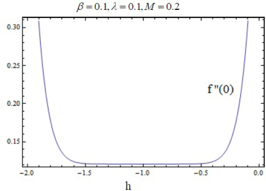
hf curve for functions f for 20th-order of HAM approximations.
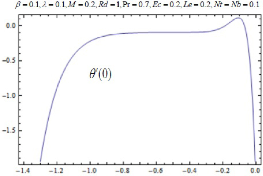
hθ curve for functions θ for 20th-order of HAM approximations.
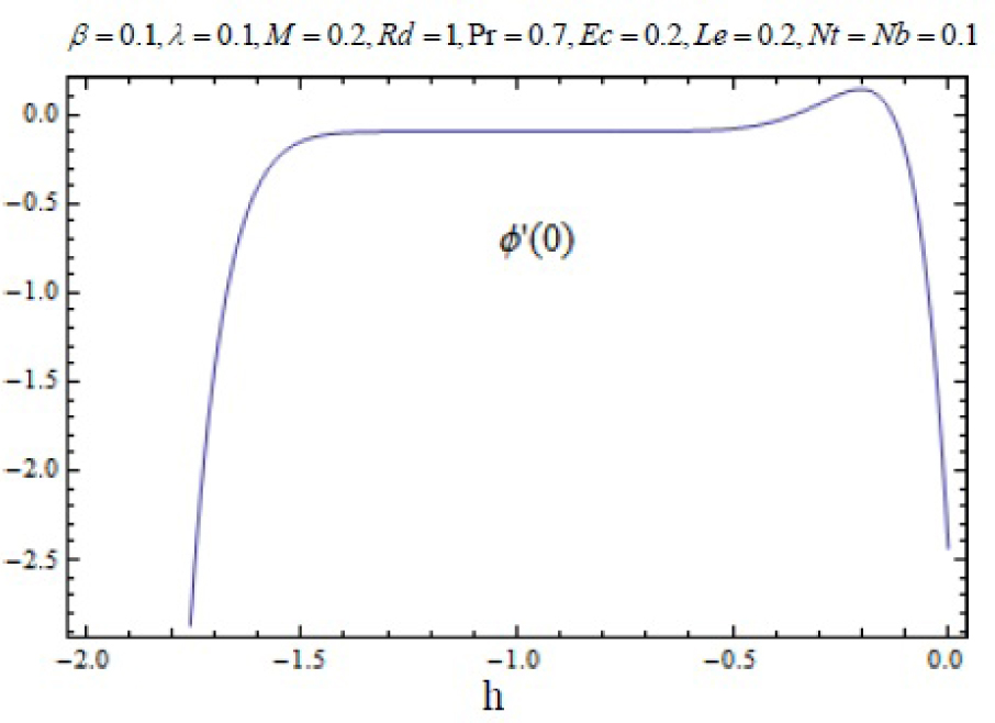
hϕ curve for functions ϕ for 20th-order of HAM approximations.
Convergence of series solution for different order of approximations β = 0.1, λ = 0.2, M = 0.2, Pr = 7, Le = 1.2, Nt = Nb = 0.1, Ec = 0.1, Rd = 0.1, ħf = −0.8, ħθ = −0.55 and ħφ = −0.7
| Order of Approximation | −f″(0) | −θ′(0) | −φ′(0) |
|---|---|---|---|
| 1 | 2.57333 | 0.888235 | 2.03667 |
| 3 | 2.53480 | 0.888136 | 2.04223 |
| 5 | 2.53266 | 0.887391 | 2.04361 |
| 10 | 2.53252 | 0.887262 | 2.04386 |
| 15 | 2.53252 | 0.887184 | 2.04402 |
| 20 | 2.53252 | 0.887102 | 2.04022 |
| 23 | 2.53252 | 0.887102 | 2.04022 |
| 25 | 2.53252 | 0.887102 | 2.04022 |
| 30 | 2.53252 | 0.887102 | 2.04022 |
Numerical values of the skin friction coefficient-f″(0) for various values of β, λ and M.
| λ | β | M | −f″(0) |
|---|---|---|---|
| 0 | 0.2 | 0.2 | 1.33216 |
| 0.1 | 1.26613 | ||
| 0.2 | 1.18392 | ||
| 0.1 | 0.4 | 0.2 | 1.01326 |
| 0.6 | 1.12364 | ||
| 0.8 | 1.24142 | ||
| 0.1 | 1 | 0.1 | 0.93624 |
| 0.3 | 1.10245 | ||
| 0.5 | 1.15243 |
5 Results and Discussions
In this work, we employed the similarity transformation to convert the governing two-dimensional partial differential equations of velocity, temperature and nanoparticles concentration to ordinary differential equations for radiative electrically conducting fluid with viscous dissipation in an impermeable surface. The HAM has been successfully applied to compute the semi-numerical solution under appropriate boundary conditions. Numerical computations of results are demonstrated in Figures 5–22 for velocity, temperature and nanoparticles concentration for various values of Magnetic parameter M, Prandtl number Pr, heat source/sink parameter A, Eckert number Ec, Deborah number β, ratio of relaxation to retardation time parameter λ, radiation parameter Rd, Brownian motion parameter Nb, thermophoresis parameter Nt and Lewis number Le. Fig.5 exhibits the variation in velocity f′(η) for different values of magnetic parameter M. It has been shown that the increase in magnetic field parameter M reduces the velocity. As M increases, a resistive force like a drag force is produced, which is called a Lorentz force. The Lorentz force retards the force on the velocity which slows down its motion. Therefore the velocity decreases with the increase of magnetic field parameter M. In Figure 6, a similar behavior on the velocity profile for different values of λ can be noticed. Since for the larger value of λ the boundary layer thickness is decreases which affect the motion of the fluid within the boundary layer region. Thus increases of λ, the velocity decreases. Similarly in Fig. 7 for various values of Deborah number β, the velocity profile f′ is observed. Since Deborah number β is proportional to λ, therefore with increases of β, velocity decreases. In Fig. 8, effects of Thermophoresis parameter Nt with temperature profile is observed. It has been seen that with an increase of Nt, the temperature is also increases. This is due to the fact that the larger values of thermophoresis parameter Nt, produces the enhancement in the thermophoresis force which tends to move the nanoparticles from hot surface to cold one. Therefore the heat transfer is increases in boundary layer region for nanoparticles. In Fig. 9, effects of Brownian motion parameter Nb with temperature profile is analyzed. It has been noticed that as Brownian motion parameter Nb increases, the mass diffusivity increases which leads to the increases of the temperature profile in the boundary layer region. In Fig. 10, it is analyzed that the temperature is decreases with increase the Lewis number Le. This is due to the fact that Le number contains the Brownian diffusivity coefficient DB which associates with the Brownian motion parameter Nb. Since the enhancement in Lewis number, decreases the thermal diffusivity of the boundary layer thickness causes to slow down the velocity in the boundary layer region. Fig. 11 represents the effects of Prandtl number Pr to temperature. It has been seen that the increases of Pr decreases the thermal boundary layer thickness, which lower the temperature within the boundary layer region. In Fig. 12, it is observed that the temperature profile is increases with increases of radiation parameter Rd. This is due to the fact that the larger value of radiation parameter Rd provided more heat to working fluid within the boundary layer region and is related to boundary layer thickness. Fig. 13 shows the variation in temperature for different values of magnetic parameter M. It has been concluded that the temperature increases with increases of M. This is due to the fact that magnetic parameter involves Lorentz force, higher magnetic field parameter involves the stronger Lorentz force leads to an enhancement in the temperature. In Figs (14) and (15), the variation of temperature θ (η) with respect to heat source/ sink parameter has been plotted. It shows that the temperature is increase with heat source parameter (A > 0) and decreases with heat sink parameter (A < 0) because the thermal boundary layer generates the energy and this causes the temperature in the thermal boundary layer increases with increases in A (for heat source) and decreases with decreases in A (for heat sink). Fig. 16 shows the effect of Eckert number on temperature. It has been observed that the temperature increases with increase of Ec. Larger value of Ec enhanced the heat in fluid flow within the boundary layer region. Fig. 17 represents the φ(η) for various value of Nb. It has been noticed that the concentration of boundary layer thickness decreases with increase of Nb. In Fig. 18 effects of nanoparticles concentration with thermophoresis parameter Nt is plotted. It has been visualized that the concentration profile increases with increase of Nt. This is due to fact that the larger value of Nt increases the thermophoresis force in the boundary layer region which leads to the higher nanoparticles concentration. In Fig. 19 the effects of Lewis number with nanoparticles concentration profile has been plotted. It shows that the larger values of Lewis number Le causes a reduction in the nanoparticles concentration. Therefore the nanoparticles concentration profile is decreases with increases of Le. The similar effect was found in Fig. 20 with Prandtl number Pr. In Fig. 21 we analyzed that the nanoparticles concentration profile is decreases with increase in heat source parameter. This is due to the fact that an increasing the heat source in the thermal boundary layers generates the energy in the boundary layer thickness and decrease the nanoparticles concentration. Fig. 22 shows the effect of Eckert number in nanoparticles concentration profile. It has been observed that the nanoparticles concentration profile is increases with increase of Ec, as larger value of Ec enhanced the heat in fluid flow within the boundary layer region. Also a comparative study has been made in Table 3 with HAM (present results) with previously published results.
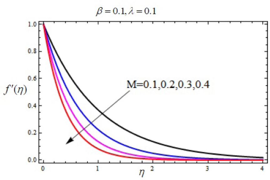
Variation of velocity f′(η) with η for several values of Magnetic parameter M.
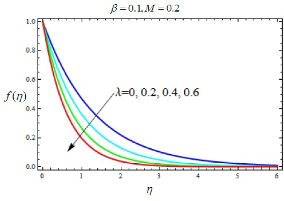
Variation of velocity f′(η) with η for several values of relaxation ratio parameter λ
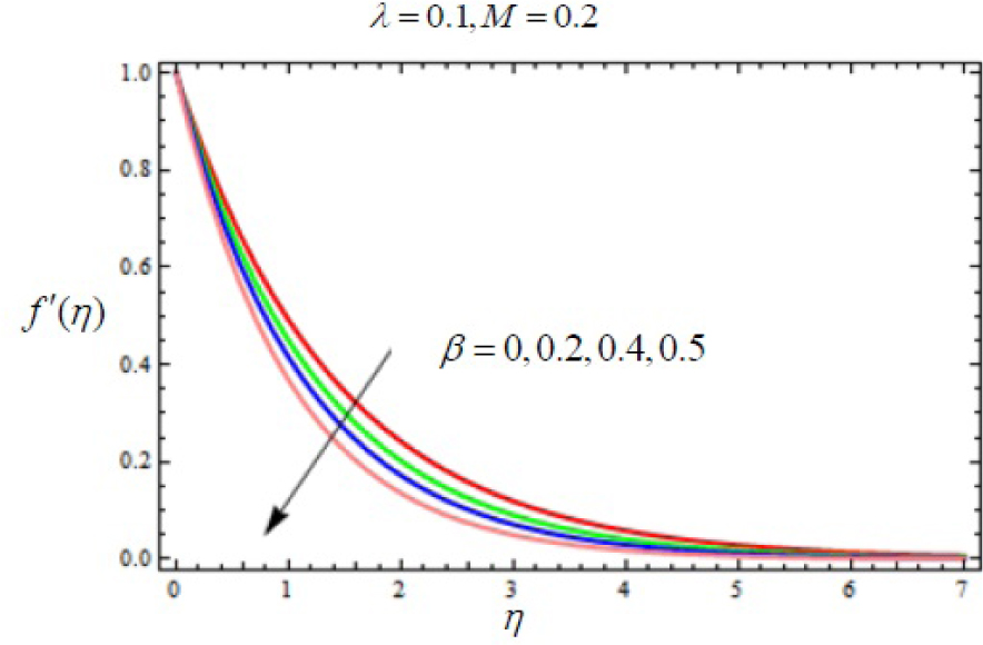
Variation of velocity f′(η) with η for several values of Deborah number λ.
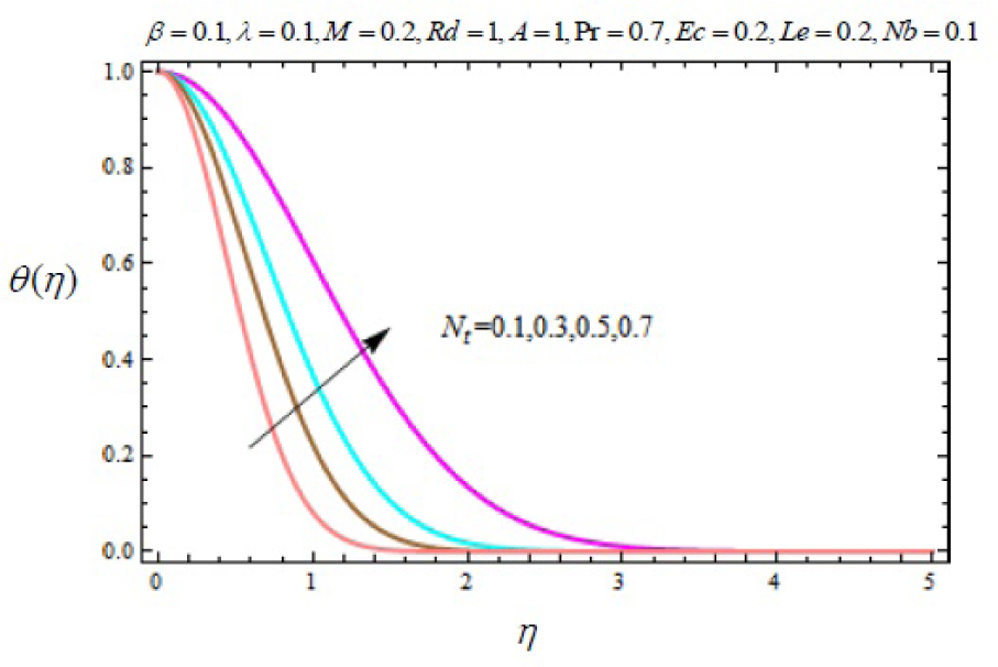
Variation of temperature profile θ (η) with η for several values of thermophoresis parameter Nt.
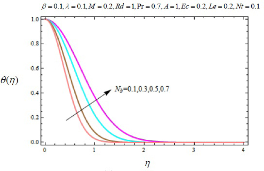
Variation of temperature profile θ (η) with η for several values of Brownian motion parameter Nb.
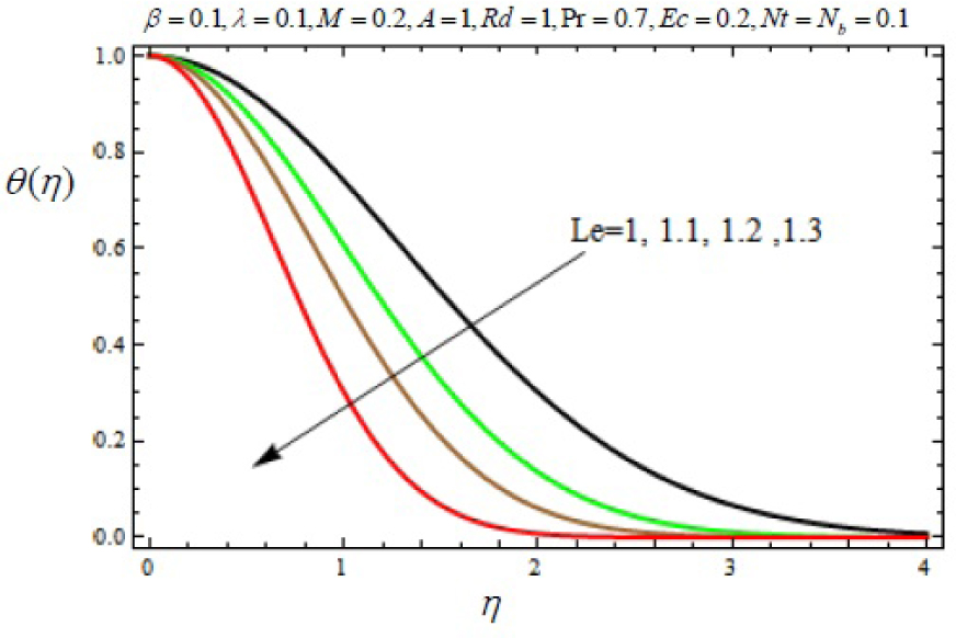
Variation of temperature profile θ (η) with η for several values of Lewis number Le.
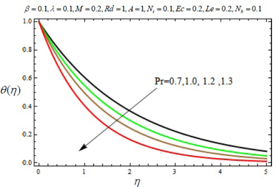
Variation of temperature profile θ (η) with η for several values of Prandtl number parameter Pr.
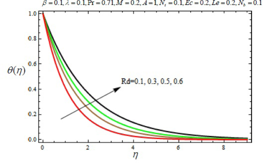
Variation of temperature profile θ (η) with η for several values of radiation parameter Rd.
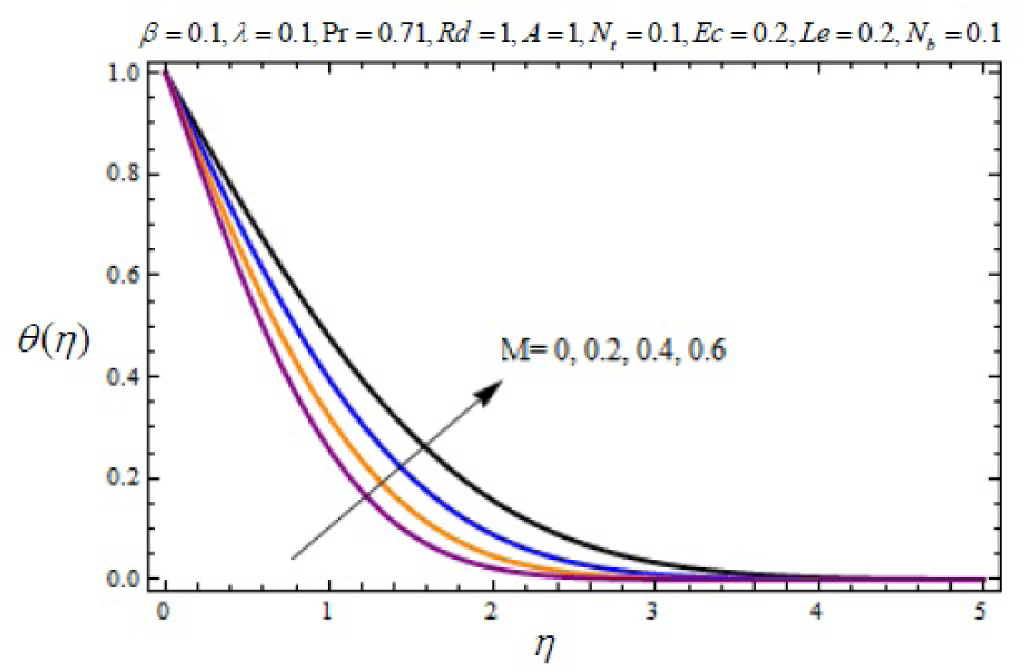
Variation of temperature profile θ (η) with η for several values of magnetic parameter M.
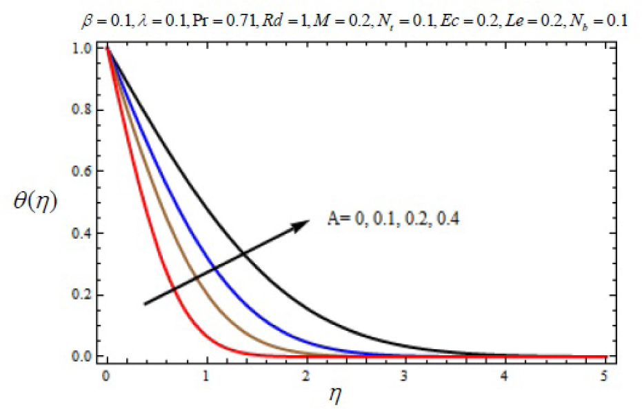
Variation of temperature profile θ (η) with η for several values of heat source parameter A > 0.
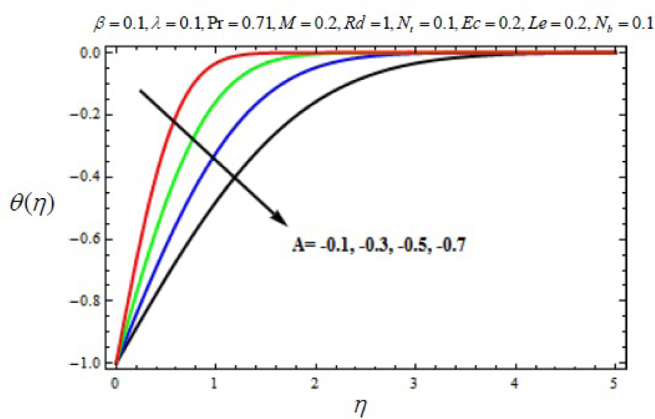
Variation of temperature profile θ (η) with η for several values of heat sink parameter A < 0.
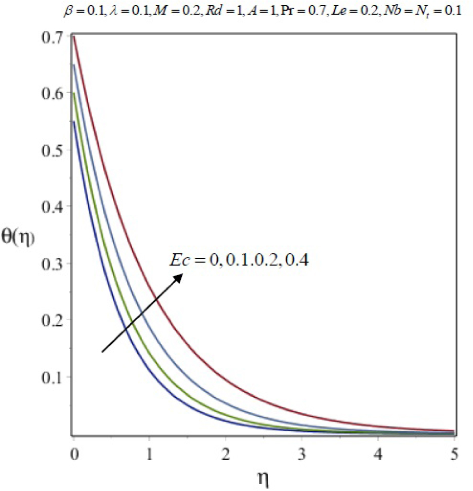
Variation of temperature profile θ (η) with η for several values of Eckert number Ec.
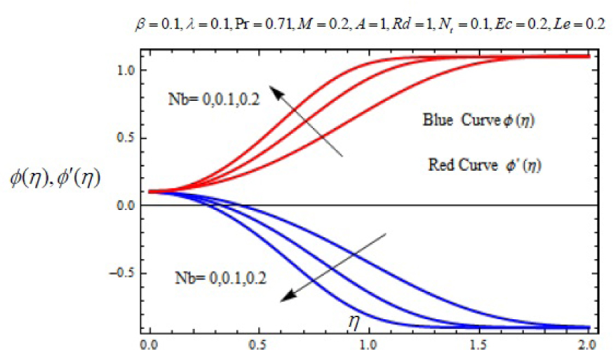
Variation ϕ(η) ϕ′ (η) with η for several values of Brownian motion parameter Nb.
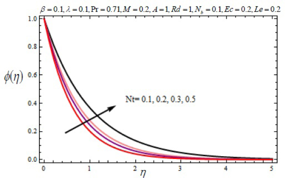
Variation of nanoparticle concentration with η for several values of thermophoresis parameter Nt.
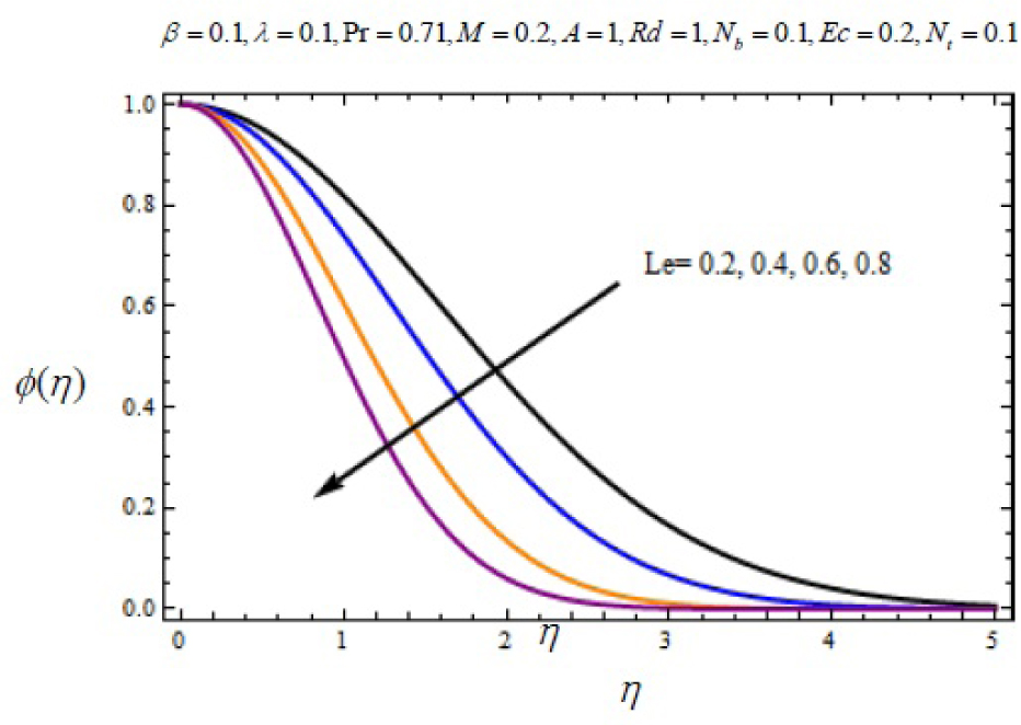
Variation of nanoparticle concentration with η for several values of Lewis number Le.
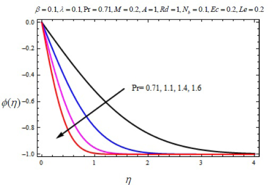
Variation of nanoparticle concentration with η for several values of Prandtl number Pr.
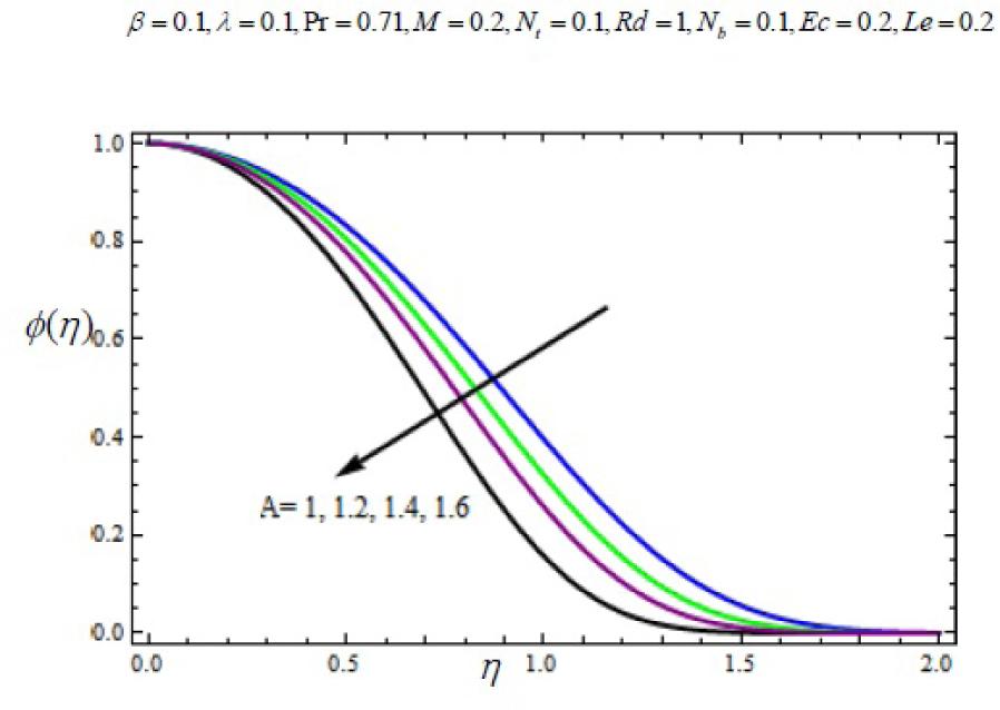
Variation of nanoparticle concentration with η for several values of Heat parameter A.
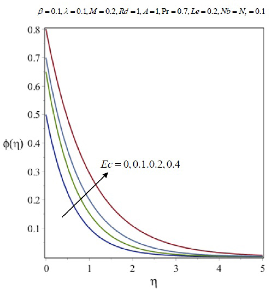
Variation of nanoparticle concentration with η for several values of Eckert Number Ec.
Comparison for HAM results of the local Nusselt number−θ′(0) in the case of β = λ = 0 Rd = Nt = Nb = 0, M = 0.1, ℏθ = −0.55, Ec = 0.1, A = 0, Le = 10
| Pr | Khan and Pop [51] | Wang [52] | Gorla and Sidani [53] | Ramesh et. al [54] | Present result |
|---|---|---|---|---|---|
| 0.7 | 0.4539 | 0.4539 | 0.5349 | 0.4582 | 0.4542136 |
| 2 | 0.9113 | 0.9113 | 0.9113 | 0.9112 | 0.9113432 |
| 7 | 1.8954 | 1.8954 | 1.8905 | 1.8953 | 1.8954124 |
| 20 | 3.3539 | 3.3539 | 3.3539 | 3.3538 | 3.3538714 |
| 70 | 6.4621 | 6.4622 | 6.4622 | 6.4621 | 6.4622357 |
Numerical values of the local Nusselt number −θ′(0) and the Sherwood number−φ′(0) for different parameters
| λ | M | β | Pr | Ec | Nt | Nb | Rd | Le | A | −(1 + 4/3R)θ′(0) | − φ′(0) |
|---|---|---|---|---|---|---|---|---|---|---|---|
| 0.1 | 0.2 | 0.1 | 1 | 1 | 0.1 | 0.1 | 0.2 | 1 | 1 | 1.2312623 | 0.7312412 |
| 0.2 | 1.2138719 | 0.7243632 | |||||||||
| 0.3 | 1.2083645 | 0.7116231 | |||||||||
| 0.2 | 0.4 | 1.2238912 | 0.7312412 | ||||||||
| 0.6 | 1.2648923 | 0.7426323 | |||||||||
| 0.8 | 1.2936912 | 0.7612104 | |||||||||
| 0.2 | 0.4 | 0.2 | 1.2138942 | 0.7312412 | |||||||
| 0.3 | 1.2021021 | 0.7136262 | |||||||||
| 0.4 | 1.1836428 | 0.7136262 | |||||||||
| 0.2 | 0.4 | 0.3 | 1.1 | 1.1986477 | 0.7312412 | ||||||
| 1.2 | 1.2138632 | 0.7230256 | |||||||||
| 1.3 | 1.3212814 | 0.7122635 | |||||||||
| 0.2 | 0.4 | 0.3 | 1.2 | 1.1 | 1.1983263 | 0.6812347 | |||||
| 1.3 | 1.1643523 | 0.6945232 | |||||||||
| 1.5 | 1.1556345 | 0.7145984 | |||||||||
| 0.2 | 0.4 | 0.3 | 1.2 | 1.3 | 0.1 | 1.2312623 | 0.6895665 | ||||
| 0.3 | 1.2068985 | 0.4289541 | |||||||||
| 0.5 | 1.1745651 | 0.1473654 | |||||||||
| 0.2 | 0.4 | 0.3 | 1.2 | 1.3 | 0.1 | 0.1 | 1.1604245 | 0.6895665 | |||
| 0.3 | 1.1385681 | 0.7264855 | |||||||||
| 0.5 | 1.0745236 | 0.7651714 | |||||||||
| 0.2 | 0.4 | 0.3 | 1.2 | 1.3 | 0.1 | 0.1 | 0.1 | 1.2345879 | 0.7568955 | ||
| 0.4 | 1.3456841 | 0.8145254 | |||||||||
| 0.7 | 1.3756125 | 0.9120478 | |||||||||
| 0.2 | 0.4 | 0.3 | 1.2 | 1.3 | 0.1 | 0.1 | 0.1 | 1.1 | 1.2524632 | 0.5123145 | |
| 1.2 | 1.2345145 | 0.6421452 | |||||||||
| 1.2 | 1.2010173 | 0.7645817 | |||||||||
| 0.2 | 0.4 | 0.3 | 1.2 | 1.3 | 0.1 | 0.1 | 0.1 | 1.1 | 1 | 1.2478956 | 0.6412656 |
| 1.2 | 1.2756845 | 0.5374589 | |||||||||
| 1.4 | 1.2814231 | 0.4546563 |
6 Concluding Remarks
In this study, the homotopy analysis method (HAM) has been successfully applied to evaluate the effects of magnetic parameter, Prandtl number, Eckert number, Brownian motion parameter, thermophoresis parameter, Lewis number and radiation parameter on the flow of an incompressible Jeffrey nanofluid over an impermeable stretching sheet. The effects of these physical parameters on the velocity, temperature and nanoparticles concentration are shown by graphs. Also a comparative study between the present analytical technique and known results is being presented in tabular form. It has been analyzed that the HAM contains an auxiliary parameter ℏ which can adjust and control the convergence region of the solution to a great extent and freely to choose any base function (exponential, algebraic, polynomials, logarithmic, trigonometrically etc.) are fully agreements with HAM. On the basis of present analyses the main outlines are listed below:
Flow velocity decreases with increase of β, M and λ.
Temperature increases with increase of Nb and Nt but decreases with the effects of Le and Pr.
For larger values of Rd and M leads to an enhancement in the temperature.
Temperature increases with heat source parameterA > 0 and decreases with heat sink parameter A < 0.
Nanoparticles concentration decreases with increases of Nb while it increases with increase of Nt.
Nanoparticles concentration profile is decrease with effects of Le,Pr and A..
Temperature and nanoparticles concentration is increases with increase of Eckert number Ec.
Nomenclature
| u, v | Components of velocity in x and y direction (m/s) |
| x | Coordinate along the stretching sheet (m) |
| y | Distance normal to the stretching sheet (m) |
| uw | Stretching sheet velocity (m/s) |
| A | heat source/sink parameter |
| c | Stretching rate |
| Cf | Skin friction coefficient |
| cp | Specific heat at constant pressure (N/m2) |
| C | Nanoparticles volume fraction |
| DB | Brownian diffusion coefficient (m2/s) |
| DT | Thermophoresis diffusion coefficient (m2/s) |
| B0 | Magnetic field strength (A/m) |
| M | Magnetic parameter |
| Nb | Brownian motion parameter |
| Nt | Thermophoresis parameter |
| Re | Reynolds’s number |
| Nux | local Nusselt number |
| Le | Lewis number |
| Pr | Prandtl number |
| Q0 | Dimensional heat generation/ absorption coefficients |
| qr | Rosseland approximation coefficient for radiation |
| qw | Surface heat flux (W/m2) |
| qm | Surface mass flux |
| Shx | Local Sherwood number |
| T | Temperature of the fluid (K) |
| Tw | Temperature of the wall (K) |
| T∞ | Ambient fluid Temperature (K) |
| k∗ | Absorption coefficient |
| Rd | Radiation parameter |
| Ec | Eckert number |
Greek Symbolss
| η | Similarity variable |
| κ | The coefficient of thermal conductivity (W/m⋅k) |
| μ | Dynamic viscosity (Ns/m2) |
| σ∗ | Stefan-Boltzman constant (S/M) |
| ν | Kinematic viscosity (Ns/m2) |
| ψ | Stream function |
| ρ | Density of the fluid (Kg/m3) |
| θ | Non-dimensional temperature |
| φ | Dimensionless nanoparticles volume fraction |
| ρf | Density of the base fluid (J/K) |
| ρp | Density of the particles (J/K) |
| λ | Relaxation to retardation times (s) |
| β | Deborah number |
| α | Thermal diffusivity |
| τw | Wall shear stress (N/m2) |
| λ1 | Relaxation time to retardation time |
| σ | Electrical conductivity |
| τ | Ratio of nanoparticle heat capacity and base fluid heat capacity |
| α | Thermal diffusivity |
References
[1] S. U. Choi, Enhancing thermal conductivity of fluids with nanoparticles, Developments and applications of non-Newtonian fluids, AJME, FED 231/ MD, 66, 99105.Suche in Google Scholar
[2] S. K. Das, S. U. Choi, W.Yu, T. Pradeep, Nanofluids: Science and Technology, John Wiley and Sons, New York, NY, USA, 2007.10.1002/9780470180693Suche in Google Scholar
[3] X. Wang and A.S. Mujumdar, A review on nanofluids-part-I theoretical and numerical investigations, Brazilian Journal Chemical Engineering, 25 (4), 613–620, 2008.10.1590/S0104-66322008000400001Suche in Google Scholar
[4] C. Yang, W. Li, Y. Sano, M. Mochizuki, A. Nakayama, On the anomalous convective heat transfer enhancement in nanofluids: a theoretical answer to the nanofluids controversy, Journal of Heat Transfer, 135(5) Article ID 54504, 9 pages, 2013.10.1115/1.4023539Suche in Google Scholar
[5] K. Jahani, M. Mohammadi, M. B. Shafii, Z. Shiee, Promising technology for electronic cooling: nanofluidic micro pulsating heat pipes, Journal of Electronic Packaging, 135 (2), Article ID 021005, 2013.10.1115/1.4023847Suche in Google Scholar
[6] J. Cai, X. Hu, B. Xiao, Y .Zhou, W. Wei, Recent development on fractal-based approaches to nanofluids and nanoparticle aggregation, International Journal of Heat and Mass Transfer, 105, 623-637, 2017.10.1016/j.ijheatmasstransfer.2016.10.011Suche in Google Scholar
[7] M. Sheikholeslami, S. A. Shahzad, magnetohydrodynamics nanofluid convection in a porous enclosure considering heat flux boundary conditions, International Journal of Heat and Mass Transfer, 106, 1261–1269, 2017.10.1016/j.ijheatmasstransfer.2016.10.107Suche in Google Scholar
[8] T. Hayat, T. Muhammad, S. A. Shehzad, A. Alsaedi, On magnetohydrodynamic flow of nanofluid due to rotating disk with slip effect: a numerical study, Computer Methods in Applied Mechanical Engineering, 315, 467–477, 2017.10.1016/j.cma.2016.11.002Suche in Google Scholar
[9] T. Hayat, T. Muhammad, S. A. Shehzad, A. Alsaedi, An analytical solution of magnetohydrodynamic Oldroyd-B nanofluid induced by a stretching sheet with heat generation/absorption, International Journal of Thermal Sciences, 111, 274–288, 2017.10.1016/j.ijthermalsci.2016.08.009Suche in Google Scholar
[10] M. S. Hashmi, N. Khan, T. Mahood, S. A. Shehzad, Effect of magnetic field on mixed convection flow of Oldroyd-B nanofluid induced by two infinite isothermal stretching disks, International Journal of Thermal Sciences, 111, 463–474, 2017.10.1016/j.ijthermalsci.2016.09.026Suche in Google Scholar
[11] M. I. Anwar, S. Shafie, T. Hayat, S. A. Shehzad, M. Z. Salleh, Numerical study for MHD stagnation point flow a Micropolar nanofluid towards a stretching sheet, Journal of The Brazilian Society of Mechanical Science and Engineering, 39, 89–100, 2017.10.1007/s40430-016-0610-ySuche in Google Scholar
[12] N. S. Akbar, S. Nadeem, C. Lee, Characteristic of Jeffrey fluid model of peristaltic flow of chime in small intestine with magnetic field, Results in Physics, 8(4), 152–160, (2013).10.1016/j.rinp.2013.08.006Suche in Google Scholar
[13] S. Nallapu, G. Radhakrishnamacharya, Jeffrey fluid flow through porous medium in the presence of magnetic field in narrow tubes, International Journal of Engineering Mathematics, 75 (5), 10–18, 2014.10.1155/2014/713831Suche in Google Scholar
[14] T. Hayat, S. Qayyum, M. Imtiaz, A. Alsaedi, Impact of Cattaneo-Christov heat flux in Jeffrey fluid flow with homogeneous heterogeneous reaction, Plos One 10.1371/journal.pone.0148662, 2016.Suche in Google Scholar PubMed PubMed Central
[15] J. Ahmed, A.Shahzad, M. Kan, R. Ali, A note on convective heat transfer of an MHD Jeffrey fluid over a stretching sheet, AIP Advances 5, 117117, (2015).10.1063/1.4935571Suche in Google Scholar
[16] F. Mabood, R. D. Abdel-Rahman, G. Lorenzini, Numerical study of unsteady Jeffrey fluid flow with magnetic field effect and variable fluid properties, Journal of Thermal Science and Engineering Applications, 8 (4), 10–19, 2016.10.1115/1.4033013Suche in Google Scholar
[17] T. Hayat, W. Muhammad, S. Shabir Ali, A. Alsaedi, MHD stagnation point flow of Jeffrey fluid by a radially stretching surface with viscous dissipation and Joule heating, Journal of Hydrology and Hydromechanics, 63 (4), 311–317, 2015.10.1515/johh-2015-0038Suche in Google Scholar
[18] L. J. Crane, Flow past a stretching sheet, Z. Angew. Math. Phys., 21, 645–647, (1970).10.1007/BF01587695Suche in Google Scholar
[19] B. C. Sakiadas, Boundary layer behavior on continuous solid surface, A.I.Ch.E, 7, 26–28, 1961.10.1002/aic.690070108Suche in Google Scholar
[20] R. C. Bataller, Radiation effects in the Blasius flow, Appl.Math.Comput., 198, 333–338, 2008.10.1016/j.amc.2007.08.037Suche in Google Scholar
[21] T. Fang, Similarity solutions for a moving flat plate thermal boundary layer, Acta. Mech., 163, 161–172, 2003.10.1007/s00707-003-0004-ySuche in Google Scholar
[22] B. L. Kuo, Thermal boundary layer problems in a semi-infinite plate by the differential transformation method, Appl.Math.Comput., 150, 303–320, 2004.10.1016/S0096-3003(03)00233-9Suche in Google Scholar
[23] A. P. Amir, B. B. Setareh, On the analytical solution of viscous fluid flow past a flat plate, Phys.Lett.A, 372, 3678–3682, 2008.10.1016/j.physleta.2008.02.050Suche in Google Scholar
[24] A. Pantokratoras, The Blasius and Sakiadas flow with variable fluid properties, Heat. Mass. Transfer, 44, 1187–1198, 2008.10.1007/s00231-007-0356-2Suche in Google Scholar
[25] S. Mukhopadhyay, G. C. Layek, Radiation effects on force convective flow and heat transfer over a porous plate in a porous medium, Meccanica, 44, 587–597, 2009.10.1007/s11012-009-9211-5Suche in Google Scholar
[26] C. H. Chen, Heat and Mass transfer in MHD flow by natural convection from a permeable inclined surface with variable wall temperature and concentration, Acta. Mech., 172, 219–235, 2004.10.1007/s00707-004-0155-5Suche in Google Scholar
[27] R. A. Damesh, H. M. Duwairi and M.Al-Odat, Similarity analysis of magnetic field and thermal radiation effects on force convective flow, Turk. J. Eng. Env. Science, 30, 2006, 83–89.Suche in Google Scholar
[28] A. Kaya, O. Aydin, Effects of MHD and thermal radiation on force convection flow about a permeable horizontal plate embedded in a porous medium, J. Therm. Sci. Technology, 32(1), 2012, 9–17.Suche in Google Scholar
[29] J. R. Spreiter, A. W. Rizzi, Aligned magnetohydrodynamics solution for solar wind flow past the earth’s magnetosphere. Acta Astronaut, 1(1-2), 1974, 15–35.10.1016/B978-0-08-018131-8.50005-6Suche in Google Scholar
[30] O. Nath, S. N. Ojha, H. S. Takhar, A study of stellar point explosion in a radiative magnetohydrodynamic medium, Astrophys. Space.Sci., 183, 1991, 135–145.10.1007/BF00643022Suche in Google Scholar
[31] N. F. M Noor, S.Abbasbandy, I.Hashim, Heat and mass transfer of thermophoretic MHD flow over an inclined radiative isothermal permeable surface in the presence of heat source/sink, Int.J. Heat Mass Trans., 55, 2012, 2122–2128.10.1016/j.ijheatmasstransfer.2011.12.015Suche in Google Scholar
[32] S. J. Liao, Homotopy analysis method in nonlinear differential equation, Springer, Heidelberg, Germany, 2012.10.1007/978-3-642-25132-0Suche in Google Scholar
[33] S. J. Liao, An optimal homotopy analysis approach for strongly nonlinear differential equations, Communication in Non Linear Science and Numerical Simulation, 15, 2010, 2003–2016.10.1016/j.cnsns.2009.09.002Suche in Google Scholar
[34] S. J. Liao, Advances in the homotopy analysis method, World Scientific, ISBN 978-9814551243, 2013.10.1142/8939Suche in Google Scholar
[35] F. Mabood, W. Khan, homotopy analysis method for boundary layer flow and heat transfer over a permeable plate in a Darcian porous medium with radiation effects, Journal of Taiwan Institute of Chemical Engineers, 45, 2014, 1217–1224.10.1016/j.jtice.2014.03.019Suche in Google Scholar
[36] M. H. Abolbashari, N. Freidoonimehr, F. Nazari and M. M. Rashidi, Analytical modeling of entropy generation for Casson nano-fluid flow induced by a stretching surface, Advanced Powder Technology, 26, 2015, 542–552.10.1016/j.apt.2015.01.003Suche in Google Scholar
[37] T. Hayat, T. Muhammad, A. Alsaedi, and M. S. Alhuthali, Magnetohydrodynamics three dimensional flow of viscoelastic nano-fluid in the presence of nonlinear thermal radiation, Journal of Magnetism and Magnetic Material, 385, 2015, 222–229.10.1016/j.jmmm.2015.02.046Suche in Google Scholar
[38] M. Mustafa, T. Hayat, A. Alsaedi, Unsteady boundary layer flow of nanofluid past an impulsive stretching sheet, Journal of Mechanics, 29(3), 2013, 423–432.10.1017/jmech.2013.9Suche in Google Scholar
[39] M. Turkyilmazoglu, MHD fluid flow and heat transfer due to a shrinking rotating disk, Computers and Fluids, 90, 2014, 51–56.10.1016/j.compfluid.2013.11.005Suche in Google Scholar
[40] M. M. Rashidi, S. A. Mohimanian pour, S. Abbasbandy, Analytic approximate solutions for heat transfer of a micropolar fluid through a porous medium with radiation, Communication in Non Linear Science and Numerical Simulation, 16, 2011, 1874–1889.10.1016/j.cnsns.2010.08.016Suche in Google Scholar
[41] T. Hayat, M. Ijaj Khan, A. Alsaedi, M. Imran Khan, Homogeneous- heterogeneous reaction and melting heat transfer in the MHD flow by a stretching surface with variable thickness, Journal of Molecular Liquids, 2016, Article in Press.10.1016/j.molliq.2016.09.019Suche in Google Scholar
[42] K. Sharma, S. Gupta, Analytical Study of MHD Boundary Layer Flow and Heat Transfer towards a Porous Exponentially Stretching Sheet in Presence of Thermal Radiation, International Journal of Advances in Applied Mathematics and Mechanics, 4(1), 2016, 1–10.Suche in Google Scholar
[43] K. Sharma, S. Gupta, Homotopy analysis solution to thermal radiation effects on MHD boundary layer flow and heat transfer towards an inclined plate with convective boundary conditions, International Journal of Applied and Computational Mathematics, Article in Press.10.1007/s40819-016-0249-5Suche in Google Scholar
[44] F. M. Abbasi, S. A. Shehzad, Heat transfer analysis of three dimensional flow of Maxwell fluid with temperature dependent thermal conductivity, Application of Cattaneo-Christov heat flux model, Journal of Molecular Liquids, 220, 848–854, 2017.10.1016/j.molliq.2016.04.132Suche in Google Scholar
[45] S. A. Shehzad, F.M. Abbasi, T. Hayat, A. Alsaedi, Cattaneo-Christov heat flux model of Darcy-Forchheimer flow of an Oldroyd-B fluid with variable thermal conductivity and nonlinear convection, Journal of Molecular Liquids, 224, 274–278, 2016.10.1016/j.molliq.2016.09.109Suche in Google Scholar
[46] F. M. Abbasi, S. A. Shehzad, T. Hayat, M. S. Alhuthali, Mixed convection flow of Jeffrey nanofluid with thermal radiation and double stratification, Journal of hydrodynamics, Ser B, 28, 840–849, 2016.10.1016/S1001-6058(16)60686-8Suche in Google Scholar
[47] M. Sheikholeslami, D. D. Ganji, Nanofluid flow and heat transfer between parallel plates considering Brownian motion using DTM, Computers Methods in Applied Mechanics and Engineering, 283, 651–663, 2015.10.1016/j.cma.2014.09.038Suche in Google Scholar
[48] M. M. Rashidi, E. Erfani, Analytical study of MHD stagnation point flow in porous media with heat transfer, Computers and Fluids, 40, 172–178, 2011.10.1016/j.compfluid.2010.08.021Suche in Google Scholar
[49] M. M. Rashidi, N. Laraqi, S. M. Sadri, A novel analytical solution of mixed convection about an inclined flat plate embedded in a porous medium using the DTM-Padé, International Journal of Thermal Sciences, 49, 2405–2412, 2010.10.1016/j.ijthermalsci.2010.07.005Suche in Google Scholar
[50] M. M. Rashidi, N. Kavyani, S. Abelman, M.J. Uddin, N. Freidoonimehr, Double diffusive magnetohydrodynamic (MHD) mixed convective slip flow along a radiative moving vertical flat plate with convective boundary condition, Plos One, 9(3), 120–137, 2014.10.1371/journal.pone.0109404Suche in Google Scholar PubMed PubMed Central
[51] W.A. Khan, I. Pop, Boundary-layer flow of a nanofluid past a stretching sheet. International Journal of Heat and Mass Transfer, 53 (11), 2477–2483, 2010.10.1016/j.ijheatmasstransfer.2010.01.032Suche in Google Scholar
[52] C. Y. Wang, Free Convection on a Vertical Stretching Surface, J.Appl. Math. Mech. (ZAMM), 69, 418–420, 1989.10.1002/zamm.19890691115Suche in Google Scholar
[53] R.S.R Gorla, I. Sidawi, Free convection on a vertical stretching surface with suction and blowing, Applied Science Research, 52, 247–257, 1994.10.1007/BF00853952Suche in Google Scholar
[54] G. K. Ramesh, Ali. J. Chamkha, B. J. Gireesha, Magnetohydrodynamic flow of a non- Newtonian nanofluid over an impermeable surface with heat generation / absorption, Journal of nanofluids, 3 78–84, 2014.10.1166/jon.2014.1082Suche in Google Scholar
© 2017 Walter de Gruyter GmbH, Berlin/Boston
This article is distributed under the terms of the Creative Commons Attribution Non-Commercial License, which permits unrestricted non-commercial use, distribution, and reproduction in any medium, provided the original work is properly cited.
Artikel in diesem Heft
- Frontmatter
- Chaos Suppression in Fractional order Permanent Magnet Synchronous Generator in Wind Turbine Systems
- Solution of Fifth-order Korteweg and de Vries Equation by Homotopy perturbation Transform Method using He’s Polynomial
- A study on validating KinectV2 in comparison of Vicon system as a motion capture system for using in Health Engineering in industry
- MHD Flow with Hall current and Joule Heating Effects over an Exponentially Stretching Sheet
- Solitons and other solutions to the coupled nonlinear Schrödinger type equations
- Nonlinear Dynamic Characteristics of the Railway Vehicle
- Quadratic Convective Flow of a Micropolar Fluid along an Inclined Plate in a Non-Darcy Porous Medium with Convective Boundary Condition
- Viscous Dissipation and Thermal Radiation effects in MHD flow of Jeffrey Nanofluid through Impermeable Surface with Heat Generation/Absorption