Optimizing the localization precision in coherent scattering microscopy using structured light
-
Ulrich Hohenester

 ,
Felix Hitzelhammer
,
Georg Krainer
,
Peter Banzer
und
Thomas Juffmann
,
Felix Hitzelhammer
,
Georg Krainer
,
Peter Banzer
und
Thomas Juffmann

Abstract
We employ the concept of quantum Fisher information to optimize the focused excitation fields in coherent scattering microscopy. Our optimization goal is to achieve the best possible localization precision for small scatterers located above a glass coverslip, while keeping the intensity of the total incoming excitation fields fixed. For small numerical aperture (NA) values, the optimal fields have linear or circular polarization, and the excitation beam can be well approximated by a Gaussian one. For larger NA values, the optimal beam acquires radial polarization. We show that the high localization precision can be attributed to high field strengths at the scatterer position, and correspondingly a large number of scattered and detected photons. Finally, we evaluate the performance of the optimized beams in interferometric scattering microscopy (iscat), and further optimize these fields for iscat localization using the concept of Fisher information.
1 Introduction
Coherent optical microscopy techniques, such as optical coherence tomography, holography, and interferometric scattering (iscat), have a profound impact on science and technology [1], [2]. The precision with which a scattering particle can be localized and tracked is often an essential figure of merit in these techniques.
In many modern microscopes, the noise in an image is dominated by shot-noise, and the localization precision scales as
In such cases, it is crucial to maximize the information obtained per photon. This can be assessed using the concepts of (quantum) Fisher information and (quantum) Cramer–Rao bounds [3], [7]. Substantial work has been devoted to the localization precision for incoherent light sources [8], [9], [10], [11]. Regarding coherent optical microscopy techniques, Bouchet et al. [12] quantitatively compared the phase estimation precision of various phase microscopy techniques, while related work quantified the precision achievable in estimating the position and polarizability of scattering particles [13] and extended these studies to the optical near-field [14]. Experimentally, the framework was applied to optimize axial localization in iscat [15] and off-axis iscat in the situation when defocus is not desired [16]. Similar studies were done in electron microscopy [17], [18], [19], where dose-induced specimen damage limits the spatial resolution in biological imaging.
Importantly, these studies assumed either plane-wave or scanned-focus illumination, trying to find an optimal detection modality such that the Fisher information comes as close as possible to the fundamental limit of the quantum Fisher information. This approach neglects the possibility of shaping the illumination light in order to maximize the quantum Fisher information.
The benefits of using a shaped illumination has been explored in fluorescence microscopy, in particular in the context of minflux, where it has been found that the (quantum) Fisher information per fluorescence photon can be vastly increased with an illumination featuring zero intensity at the position of the fluorophore [20], [21], [22], [23]. Positioning the illumination zero at various positions close to the fluorophore enables the precise localization based on a few detected fluorescence photons. Importantly, the information is quantified per fluorescence photon, as it is the number of emitted photons that limits estimation precision, determines phototoxicity, and limits observation time due to bleaching.
Recently, shaped illumination has also been used to identify optimal coherent measurements on scatterers inside highly scattering media [24], [25]. This work also led to optimal states for the optical manipulation of particles [26] and to a general framework of information flow [27].
Here, we study the optimization of localization precision in coherent microscopy techniques based on shaping the incoming illumination. In contrast to the existing work on fluorescence microscopy, we optimize the (quantum) Fisher information per incoming photon and not per scattered photon. This is justified in applications where phototoxicity, e.g., via the excitation of endogenous fluorophores [6], limits the illumination intensity. This regime gains more and more importance as the spatial and temporal resolution of coherent microscopy techniques is improved, often at the price of higher illumination intensities.
We first compare the two most common iscat modalities, which feature either focused excitation scanned across the sample or widefield excitation. We then optimize the illumination using a fast and powerful matrix optimization approach, which yields optimal solutions that maximize the quantum Fisher information in the collected light, or the Fisher information in a specific measurement. While the optimal solutions depend on the numerical aperture (NA) of the detection system, we find that a simple focused Gaussian beam performs close to optimally, particularly for smaller NAs. At high NAs, we find that optimized structured illumination provides a more than twofold improvement in quantum Fisher information. At very high NAs, and for particles located close to an interface (as is the case in many iscat measurements), we further find that evanescent modes also contribute significantly to the localization precision.
2 Theory
The problem of our present concern is depicted in Figure 1. An incoming light beam propagating in the backfocal plane along +z is focused onto a particle (denoted as the scatterer) located at position R 0,
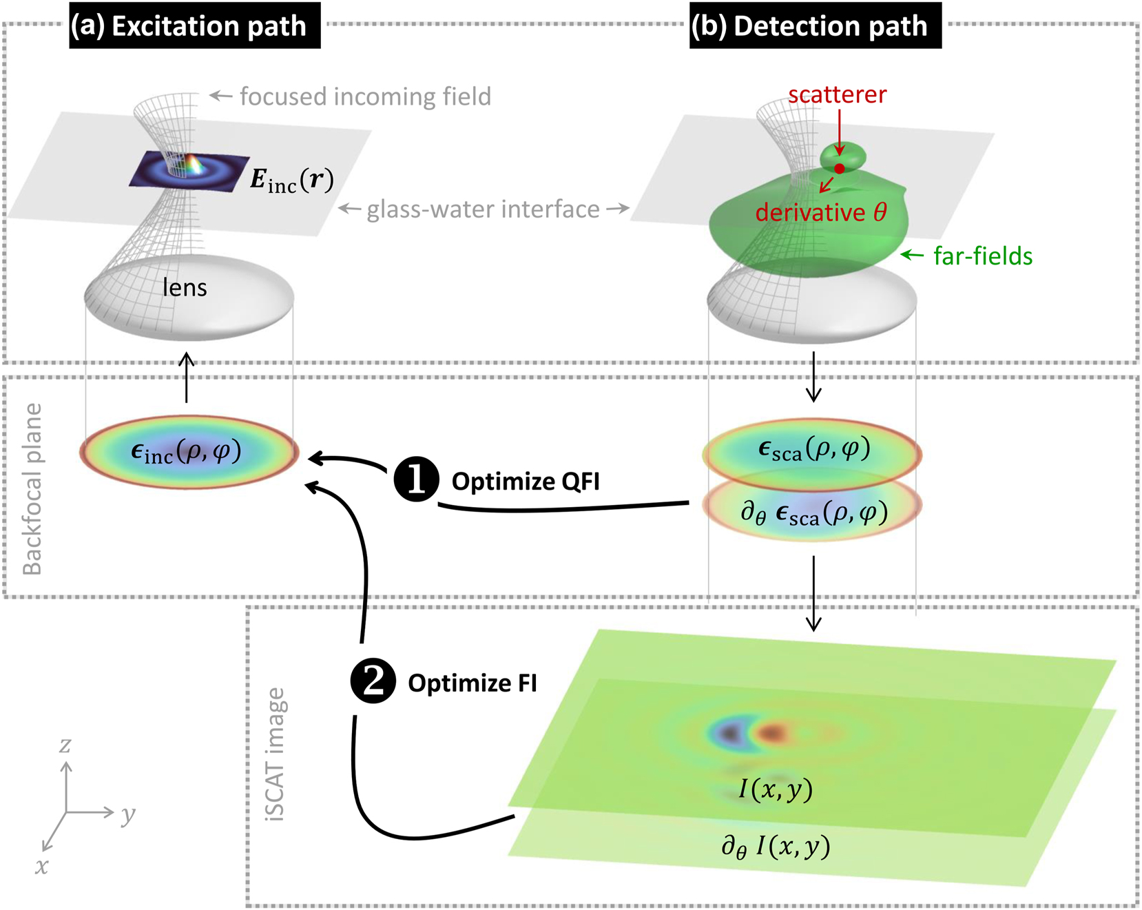
Schematics of optimization of Fisher information (FI) and quantum Fisher information (QFI) in coherence scattering microscopies. The objective of the optimization is to obtain the best localization in (1) any type of coherence microscopy and (2) interferometric scattering microscopy (iscat). (a) An incoming field
ϵ
inc propagating along +z in the backfocal plane is focused onto a glass–water interface. (b) A particle located on top or above the interface scatters light (see far-field pattern), which is collected by the same lens and transformed to a backfocal scattered field
ϵ
sca propagating along −z. Together with the incoming fields reflected at the glass–water interface (reference fields), the superimposed fields form the iscat image
We will consider the situation that the scatterer is embedded in water and is either located directly on top of a glass coverslip or sufficiently far away from it. Part of the incoming light is coherently scattered by the particle, the far-fields
F
sca propagating in the direction
Together with the reference fields E ref, which are reflected at the glass–water interface of the setup, one can compute the iscat image from
The questions we will address in this work are as follows:
What are the optimal incoming fields
What is the best possible localization precision that can be obtained on the basis of the iscat images?
2.1 Fisher information
To answer these questions, we will use the concept of the Fisher information (FI) [3], [7]. It accounts for the amount of information that the measurement data carry about an unknown parameter. Let us first consider the localization estimation using experimental iscat data. Our goal is to estimate the particle position
R
0 from the iscat images
Suppose that we have two different incoming fields
ϵ
inc at hand. Through the Fisher information, we can determine which field provides greater sensitivity to the parameter of interest and should thus be used in noisy experiments. In the language of probability theory,
which accounts for the (normalized) change of
A large Fisher information indicates that the measurement data change significantly upon variation of θ
i
, and thus a high localization precision can be obtained in experiment. The expectation value
where the sum extends over the pixels x, y of the image detector and Δx, Δy denote the pixel size. We have introduced a normalization factor N that is conveniently set to the intensity of the scattered fields in the backfocal plane [13] (proportional to the number of detected photons). In the study of structured light fields, we proceed somewhat differently and use instead the intensity of the incoming fields (proportional to the number of incoming photons). From the Fisher information, one can define the Cramér–Rao bound on the standard deviation of any unbiased estimator for the parameter θ i per incoming photon as
The equality sign should be understood as an assignment of notation, where
where Ninc and Ndet denote the numbers of incoming and detected photons, respectively.
2.2 Quantum Fisher information
We can extend the concept of Fisher information to the quantum regime, where the quantum Fisher information (QFI) quantifies the sensitivity of a quantum state to changes in the parameter of interest, independent of any specific measurement scheme. In other words, it doesn’t rely on iscat or any other variant of coherence microscopy but addresses the question what could be obtained under the best possible measurement conditions. As has been shown in Ref. [24], for coherent scattering measurements (as studied in this work), the quantum Fisher information can be obtained from the scattered fields in the backfocal plane through
where ρNA is the cutoff radius for a given numerical aperture (NA) of the lens. Below we will show that these optimized fields can be obtained in a computational approach through a matrix diagonalization, which makes the approach extremely simple and powerful. In the same way as for the Fisher information discussed above, we can introduce a quantum Cramér–Rao bound
which sets a lower bound on the standard deviation of the best possible estimator for the parameter θ i and per incoming photon.
2.3 Normalization of Fisher information
When normalizing the Fisher information, we can do so in many ways. We can normalize per incoming photon, per scattered photon, per absorbed photon, or per detected photon. In order to choose the right normalization, we have to know what limits the accuracy in our measurements experimentally. Here are some examples:
If the number of photons per time available from the light source is limiting the experiments, then one should optimize per incoming photon. This is rarely a problem these days.
In fluorescence microscopy, it is known that the excitation, relaxation, and photobleaching of the fluorophores lead to reactive oxidative species that can harm live cells and organisms [30]. It is, therefore, often appropriate to maximize the Fisher information per excitation–relaxation cycle, i.e., per emitted fluorescence photon.
In coherent microscopy, phototoxicity is often less of a problem, and many experiments are limited by the low photon detection rate, i.e., the number of photons that can be recorded per pixel per frame. In this case, one should normalize per detected photon, which we did in a previous paper [13].
However, even if an imaging modality is based on elastic scattering, the illumination light can still cause phototoxicity, e.g., due to molecules that absorb light. A common example is the imaging of live-cells with blue or UV light, but even infrared light can inactivate bacteria at moderate intensities [31], which are commonly applied in coherent scattering microscopy. In this case, it is then again appropriate to normalize per incoming photon. With coherent scattering imaging being done at faster and faster framerates, requiring higher and higher excitation intensities [4], this regime will become more prominent in the future, which is why we chose this normalization for our manuscript.
2.4 Computational approach
In our computational approach, we adopt the coherent scattering microscopy add-on [28] to the generic Maxwell solver toolbox nanobem [32], [33]. Contrary to our previous work, we are only interested in small and weak scatterers that can be described well in the dipole approximation [34] without solving the full Maxwell equations for the dielectric particle. All our simulations can be broken down into the following steps (see [28] for a more detailed discussion).
The incoming fields induce an oscillating dipole moment p = α E of the scatterer, where α is the polarizability of a sphere [34], which produces outgoing waves
The scattered fields are collected by a lens and converted to fields ϵ sca(ρ m , φ m ) propagating in the backfocal plane along −z. Again, the fields are given on a polar grid.
We are now ready to compute both types of Fisher information. We first approximate the derivative of the scattered fields in the backfocal plane using finite differences.
with a similar expression for
where w m are the quadrature weights adopted in the numerical approach, such as Gauss–Legendre weights in this work. We next use that in linear response the scattered fields can be related to the incoming fields through a transition matrix T ( θ ),
where m labels the polar grid points and we have introduced the short-hand notation ϵ m = ϵ (ρ m , φ m ). In computing the quantum Fisher information, we set the normalization factor to the intensity of the incoming fields, N = ∑ m w m | ϵ inc,m|2, and obtain from Eq. (9)
with the diagonal matrix w mm′ = w m δmm′. Equation (13) is a quadratic form, and the best possible fields are obtained from the solutions of the generalized eigenvalue problem (see [24] for a related approach)
The eigenvectors associated with the largest eigenvalue Λ = QFI(θ
i
) are the optimized fields
where R 0 = (X0, Y0, Z0) is the particle position. Using this expression, in the diagonalization, we then optimize the localization precision for all three spatial directions rather than a single one, where γ is a scaling parameter that weights the relative importance for localization along X0, Y0 with respect to Z0. Quite generally, one could also consider off-diagonal contributions to the Fisher matrix, but for the setups considered in this work, they turned out to be of minor importance and were thus neglected.
For iscat experiments, the optimization of the FI(θ i ) in Eq. (5) cannot be expressed as a quadratic form in the incoming fields and cannot be converted to an eigenvalue problem or something related. We thus have to proceed differently. In our computational approach, we start from some initial guess and maximize the Fisher information in an iterative fashion using the fminunc function of matlab. More details about our approach will be given in Section 3.3.
3 Results
Using the formalism presented in Section 2, we performed optimizations of the Fisher information for a weak scatterer located on top of a glass–water interface or placed sufficiently far away from it. The pertinent simulation parameters are listed in Table 1. We consider a weak scatterer, which we model as a sphere with a diameter of 20 nm and a refractive index of 1.58, representative for biological samples [37]. In our simulations, we employ the dipole approximation for the light scattering of the particle, which is then fully characterized by its polarizability. For this reason, the precise particle parameters are of no particular importance in our simulation results, apart from a constant prefactor for the total scattered fields that are proportional to the polarizability of the scatterer. We correspondingly report the Fisher information and all related quantities in arbitrary units throughout. Our results would not change dramatically when the particle shape slightly deviates from a spherical shape, at least for aspect ratios close to one. For the small permittivity contrasts considered in this work, multiple scatterings between the particle and the substrate are expected to be of minor importance, although they could be added in our approach along the lines discussed in Ref. [28]. Note that for the scatterer on top of the glass–water interface, we use an additional gap distance of 5 nm, but the results would remain practically unaltered when locating the particle directly on the interface. In all our simulations, we use our previously published software nanobem [28], [38].
Simulation parameters used in this work.
| Symbol | Value | Description |
|---|---|---|
| λ | 520 nm | Light wavelength in vacuum |
| NA | 1.0–1.45 | Numerical aperture |
| n ρ , n ϕ | 25–100 | Discretization points for lenses |
| n glass | 1.50 | Refractive index for glass |
| n water | 1.33 | Refractive index for water |
| n part | 1.58 | Refractive index for particle |
| d | 20 nm | Diameter of particle |
| z 0 | 5 nm, 1 μm | Particle–interface distance |
3.1 A first glimpse on optimization
In order to get a better feeling of what we are aiming for, in Figure 2, we plot the field intensities and phase distributions for three incoming fields, namely a plane wave impinging from below on the glass–water interface (left, a–c), a focused Gauss beam (middle, a’–c’), and an optimized beam (right, a”–c”) that is obtained from the maximization of the quantum Fisher information in Eq. (14). For the plane wave polarized along x, we observe below the interface the interference between the primary incoming wave propagating in the +z direction and the secondary wave reflected at the interface propagating in the −z direction. In the middle panels, we show the results for a Gaussian incoming field with circular polarization
which becomes focused through a lens with a numerical aperture of NA = 1.4 (see Figure 1). E0 is chosen such that the field strengths of the plane wave and the focused Gauss beam are the same at the scatterer position R 0. When comparing the quantum Fisher information values of Eq. (9), reported at the bottom of Figure 2, we observe that the focused Gauss beam has a better localization precision. In the right panels, we show that the localization precision can be further boosted through an optimization of the quantum Fisher information. This shows that, with constant electric field at the scatterer position, a narrow illumination beam yields the highest quantum Fisher information regarding localization in the scattered light. This result has to be met with caution. First, with a tightly focused illumination beam, it will be difficult to tune the scattered and the reference fields separately (e.g., via defocusing for phase, or via the use of attenuators for amplitude tuning), potentially leading to the Fisher information being significantly smaller than the quantum Fisher information. Second, if a focused beam is scanned in order to image an extended field of view, the average quantum Fisher information will probably be lower for the focused beams.
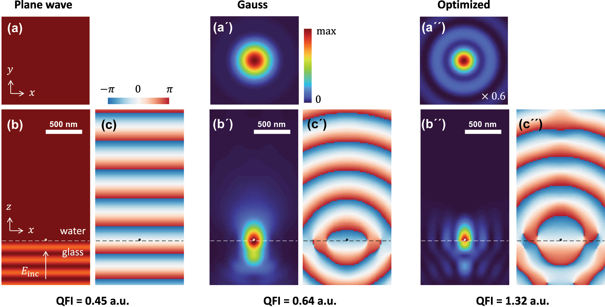
Intensity and phase maps for coherent scattering microscopy using a plane wave (left), a focused Gaussian beam (middle), and an optimized beam (right). The focusing lens has a numerical aperture of NA = 1.4. We report the intensity of the incoming beam in the (a) xy (z = 0) and (b) xz-plane. The glass–water interface is indicated by a dashed line, and we also show the scatterer with a diameter of 20 nm located on top of the interface. Panel (c) reports the phase map for the incoming field Einc,x. Below the figures, we report the quantum Fisher information in arbitrary units. In the simulations, we use the same incoming intensities for the Gauss and optimized beam, the field strength of the plane wave is chosen such that it equals that of the Gauss beam at the position of the scatterer. The intensity of the optimized beam is scaled by a factor of 0.6.
3.2 Optimization of quantum Fisher information
In this section, we provide a detailed discussion of the optimized structured-light beams and the resulting quantum Fisher information values. We start from Eqs. (14a) and (15) with γ = 0.2 and comment on the importance of the scaling parameter γ in Appendix A. Figure 3 shows the optimized incoming modes in (a, a*) the backfocal plane and (b, b*) the plane where the scatterer is located. The left panels (a–c) report results for the scatterer on top of the interface, and the right ones (a*–c*) for a particle–interface distance of 1 μm. In the first rows of panels (a, a*) and (b, b*), we show results for a numerical aperture of NA = 1.2, and in the second rows for NA = 1.4.
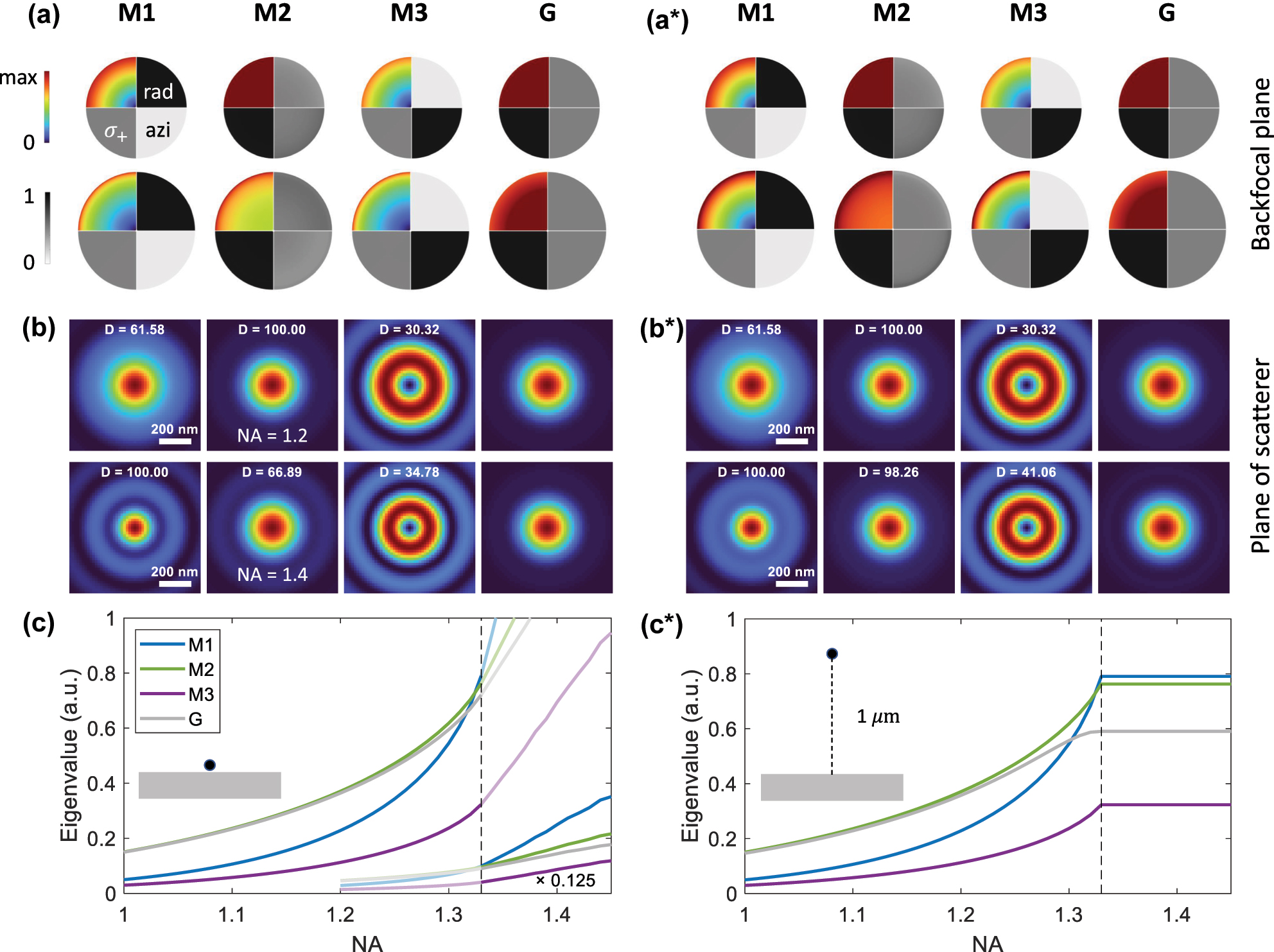
Modes with optimized quantum Fisher information in (a, a*) backfocal plane and (b, b*) plane where the scatterer is located, and for scatterer (a, b) on top of glass–water interface and (a*, b*) located 1 μm away from the interface. The colored quarter-disks in (a, a*) show the intensities of the incoming beams, and in the grayscale quarter-disks, we project the field-distribution onto radial, azimuthal, and circularly polarized (σ+) unit vectors. The optimized modes exhibit (M1) radial, (M2) circular, and (M3) azimuthal polarization. For comparison, we also show a (G) Gaussian mode with circular polarization. The modes in the first and second rows of panels (a, b) show results for numerical apertures of 1.2 and 1.4, respectively. (c, c*) Eigenvalues of Eq. (14), which are proportional to the quantum Fisher information, as a function of NA for different modes. For the particle on top of the substrate and for large NA values, we scale the eigenvalues by a factor of 0.125 for better visibility.
Although in our optimization approach we do not enforce any symmetry constraints, the problem under study exhibits cylinder symmetry, mainly due to our consideration of small particles (note that things would strongly differ for larger particles [39]), and thus also the optimized solutions exhibit such symmetry. For this reason, we plot in Figure 3(a) the field intensities and polarization properties only in a quarter of a disk. The colored parts (upper-left quarter-disks) report the intensities of the optimized incoming fields ϵ inc(ρ, ϕ) in the backfocal plane. In the remaining quarter-disks, we project the fields onto unit polarization vectors u λ through
where the degree of polarization
Figure 3(b) and (b*) shows the intensities of the focused fields E inc in the plane of the scatterer that is located in the center of the panels. The radial mode M1 has a maximum intensity at the particle position R 0, where the electric field points in the z-direction, contrary to the azimuthal mode that has zero electric field intensity there. The intensity maxima of M2 and G are located at R 0, and the electric field lies in the xy-plane and has a circular polarization. In the panels, we also report the relative importance of the eigenvalues D = 100 Λ/Λmax, with a factor of D = 100 corresponding to the largest eigenvalue.
The dependence of the eigenvalues (that equals the quantum Fisher information) on the numerical aperture is shown in Figure 3(c) and (c*). For NA values below say 1.3, the circular mode M2 performs best; however, the Gaussian mode with our ad-hoc choice of a unit variance performs almost equally well. This is remarkable. We have developed a framework for optimizing the quantum Fisher information, enabling the computation of fields that maximize localization precision, and have not imposed any constraints on the shape of the incoming fields ϵ inc. Also their polarization properties have been left arbitrary. Nevertheless, the diagonalization approach comes up with four “boring” modes to be classified in terms of radial, circular, and azimuthal polarization. And for NA ≤ 1.3, the performance is even comparable to that of a simple Gaussian beam. Alas, we had hoped for better.
Things change for larger NA values, in particular for the scatterer on top of the substrate. Here, the radial mode M1 has the largest eigenvalue, which further increases for NA values that are large enough to support incoming waves with propagation angles above the cutoff value for total internal reflection (TIR). These wave components generate evanescent fields above the glass–water interface, which induce a strong dipole moment of the scatterer in z-direction and correspondingly an efficient scattering into the substrate. Indeed, when comparing panels (c) and (c*) for the scatterer on top and above the interface, we observe that for the large gap distance of 1 μm evanescent waves play no role and the eigenvalues remain bound to those NA values where TIR waves can be excited. It is thus the appearance of evanescent waves that boosts the localization precision. We note that evanescent waves not only play a role for radial polarization but also for all other modes, see Figure 3(c), although the localization enhancement is by far the strongest for the M1 mode.
In Appendix A, we show that the optimized fields also perform well for particles located in the vicinity of the spot for which they have been optimized. We also demonstrate that the precise value of the scaling parameter γ is not overly important.
Figure 4 provides a deeper insight into the contributions to the quantum Fisher information. The transition matrix in Eq. (12) can be conveniently decomposed into two contributions
where T inc( θ ) accounts for the transition from the incoming fields to the scatterer, and T sca( θ ) for the transition from the scatterer to the backfocal plane. The terms entering Eq. (15) can then be decomposed into the contributions
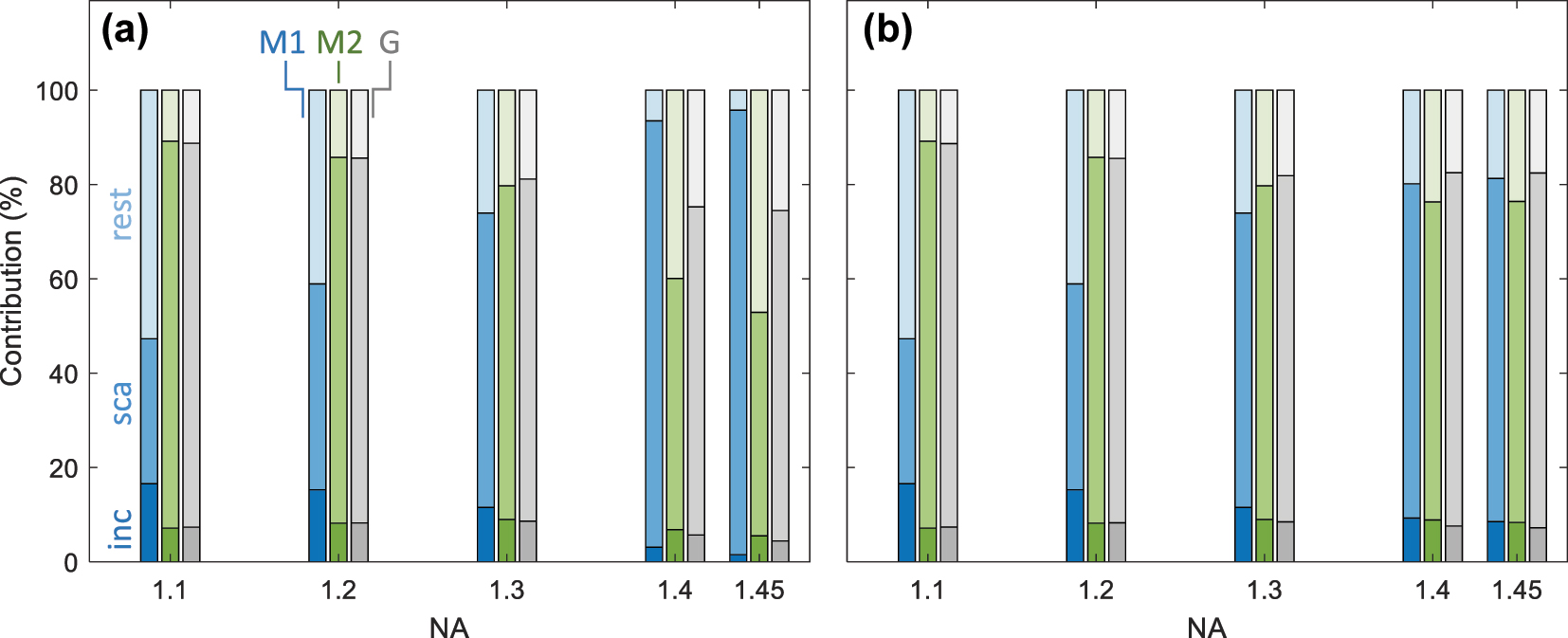
Incoming, scattered, and remaining contributions of quantum Fisher information for different modes and NA values, see Eq. (19), and for (M1) radial, (M2) circular, and (G) Gaussian mode. We show results for the scatterer located (a) on top and (b) 1 μm away from the interface. For details, see text.
The expression in the first line accounts for the change of the incoming fields upon variation of θ i while keeping the scattering properties fixed (incoming contribution). This contribution is expected to be large for excitation fields with high spatial gradients, where a slightly displaced particle is excited differently. The expression in the second line accounts for the modified scattering properties for fixed incoming fields (scattering contribution). Likewise, the expressions in the third and fourth lines account for mixed contributions (rest). The relative importance of the respective contributions is reported in Figure 4. Importantly, for the best modes (M2 for small NA values, M1 for larger NA values), the largest contribution is the scattering one. This shows that the high localization precision of these modes is not due to the fact that the scatterer is excited by a highly structured light field where the excitation properties change significantly when varying the particle position. Rather the scattering channel plays the important role, where a change of the particle position R 0 leads to far-field modifications that carry the information about R 0. For large NA values and the particle on top of the substrate, also the evanescent fields at R 0 are transformed into waves propagating toward the lens, which then carry additional information about R 0.
The above discussion explains why certain modes are better suited for particle localization than others: the optimized modes essentially maximize the field strength (and correspondingly the induced dipole moments) at the scatterer positions. Depending on the NA value of the focusing lens, the induced dipole moments are either located in the interface plane (M2) or perpendicular to it (M1). At the same time, the distribution of the incoming fields is surprisingly simple and could be approximated by even simpler Gaussian mode profiles with circular or radial polarization without significantly deteriorating the localization precision.
3.3 Optimization of Fisher information
So far we have computed the incoming fields that optimize the quantum Fisher information of Eq. (14). We should stress that our approach is quite general, and correspondingly the localization precision bounds obtained are generally valid for any type of coherent localization microscopy. However, it is not clear whether these bounds can indeed be reached in actual experiments and, if this is the case, which technique and localization protocol should be used. In this section, we make a first step in answering these questions and evaluate the localization performance of iscat. We start by comparing the quantum and iscat Cramér–Rao bounds, Eqs. (7) and (10), using the fields obtained from the optimization of the quantum Fisher information, and then continue to optimize directly the iscat Fisher information of Eq. (6). In our following discussion, we only present results for a scatterer located on top of the interface. As has been shown above, for smaller NA values, say below 1.3, the results for scatterers on top and away from the interface are very similar. In setups with larger NAs additionally evanescent waves can be excited, which are of importance only for scatterers on top of the interface.
Figure 5 shows results for the iscat Cramér–Rao bounds, which are obtained by starting from the optimized solutions of the quantum Fisher information and maximizing the Fisher information in Eq. (5) using an iterative procedure. Similar results were also obtained when starting from a random guess for the incoming fields. Let us first concentrate on the dashed lines in panels (c), which report the NA dependence of
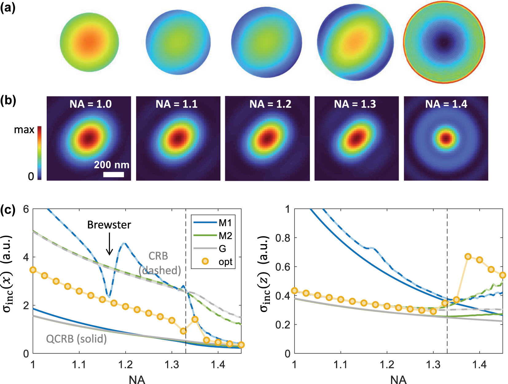
Optimization of the Fisher information for particle localization in iscat, see Eq. (6), and for a scatterer located on top of a glass–water interface. Electric field intensity in (a) backfocal plane and (b) plane of scatterer, and for the different NA values reported in the panels. (c) Localization precision along x (left panel) and z (right panel) as a function of the NA. The solid lines report the quantum Cramér–Rao bounds and the dashed lines the iscat Cramér–Rao bounds, as obtained from Eq. (7) for the optimized fields computed from the solutions of Eq. (14). The symbols show the bounds as obtained from the optimization of the Fisher information (γ = 0.2). For details, see text.
When comparing the quantum (solid lines) and iscat (dashed lines) Cramér–Rao bounds, one observes for small NA values a ratio of about three for the localization precision along x (left) and a significantly smaller ratio for z (right). This finding is in agreement with those for plane-wave excitations [13], [40]. For NA values above 1.3, the ratio of the localization precision along x decreases, with values of 2.2 for NA = 1.4 and 1.7 for NA = 1.45. At the same time, the localization precision along z deteriorates.
We additionally performed optimizations for the iscat Fisher information given in Eq. (6). In the optimizations, we expanded the incoming fields in a basis obtained from the solutions of Eq. (14), keeping the 25 modes with highest eigenvalues, and optimized the expansion coefficients in an iterative procedure such that the Fisher information becomes maximized. We started the optimization either with the mode associated with the highest eigenvalue or with random expansion coefficients, obtaining similar results in both cases. Quite generally this doesn’t mean that our optimization approach provides us with the global maximum; however, it shows that it is not overly sensitive to the initial guess for the incoming fields.
The symbols in Figure 5 show the Cramér–Rao bounds obtained from these optimizations. One observes that
4 Summary and discussion
In summary, we have investigated the optimization of particle localization precision based on coherent scattering using structured light. Within the framework of the quantum Fisher information, we have derived a generalized eigenvalue problem whose solution provides us with the optimized excitation fields. In the context of the localization of small scatterers, these fields have relatively simple distributions and polarization properties and could even be replaced by more simple Gaussian fields. We have shown that the main physical mechanism of the optimization is the maximization of the number of scattered photons. In the context of interferometric scattering microscopy, we have discussed that the optimized fields outperform plane waves if the scatterer is prelocalized to within the focal spot, and the performance can be boosted through a further optimization based on the Fisher information.
Shaping the excitation light field, especially using radial polarization and high-NA focusing, can significantly improve localization precision in coherent microscopy. This has practical implications for enhancing localization precision in iscat experiments, particularly in label-free single-particle tracking, where nanometer-scale positional accuracy is essential. Importantly, our optimization suggests that, when phototoxicity is a problem, tracking should be done with focused light intensity, and not with wide-field illumination. Beyond these, the approach could also benefit biological imaging of nanoscale structures or dynamic processes where minimizing photon flux while maximizing spatial precision is critical.
For the generation of light beams featuring a ring-like intensity distribution and a radial or azimuthal polarization, standard liquid-crystal–based q-plates can be utilized, resulting in high-quality cylindrical vector beams. The use of spatial light modulators or bespoke metasurfaces for beam-shaping would allow for more complex beam shaping, not only structuring the polarization state but also the required intensity to match more closely the modes with optimized Fisher information.
The probably most appealing part of our work is the optimization of the quantum Fisher information through the solution of a generalized eigenvalue problem, following the seminal work of Ref. [24]. This approach not only provides us with a simple and versatile scheme to obtain general and definite answers, it also paves the way for a variety of other investigations using different optimization goals. In this context, the central ingredients are the matrices entering the eigenvalue problem, which encode the goals we are seeking for.
In this work, we have been seeking for the optimization of the incoming fields that allow for the best possible localization, subject to the constraint that the power of the incoming fields is kept constant. The power constraint could be modified, for instance such that the quantum Fisher information per detected photon is maximized, as is usually done in fluorescence microscopy, see also the introductory discussion. Here, the optimal incoming beam becomes the azimuthal mode, which is extremely sensitive to variations of the scatterer position located in close vicinity to the vortex center, despite the fact that only very few photons are scattered.
In a broader sense, all such types of optimization in optical microscopy call for precise questions of what should be optimized and how different setups should be compared. It often only takes a small shift in the optimization goals to get completely different answers. Although this is a somewhat trivial statement, we feel that it is sometimes not fully appreciated. If applied rigorously, the (quantum) Fisher information framework provides a powerful tool and can give definite answers in the context of optical microscopy.
-
Research funding: This work was supported by the European Union (ERC, SignAlloMod, 101164135, G.K.). Views and opinions expressed are, however, those of the author(s) only and do not necessarily reflect those of the European Union or the European Research Council. Neither the European Union nor the granting authority can be held responsible for them. The financial support by the Austrian Federal Ministry of Labor and Economy, the National Foundation for Research, Technology and Development, and the Christian Doppler Research Association is gratefully acknowledged. The authors acknowledge the financial support by the University of Graz.
-
Author contributions: All authors have accepted responsibility for the entire content of this manuscript and consented to its submission to the journal, reviewed all the results, and approved the final version of the manuscript.
-
Conflict of interest: Authors state no conflicts of interest.
-
Data availability: Data underlying the results presented in this paper are not publicly available at this time but may be obtained from the authors upon reasonable request.
Appendix A: Robustness of simulation results
In this Appendix, we investigate the influence of our simulation results on the scaling parameter γ and show that the optimized fields also perform well for scatterer positions in the vicinity of the position for which the fields have been optimized.
Figure 6 shows the dependence of the quantum Cramér–Rao bound
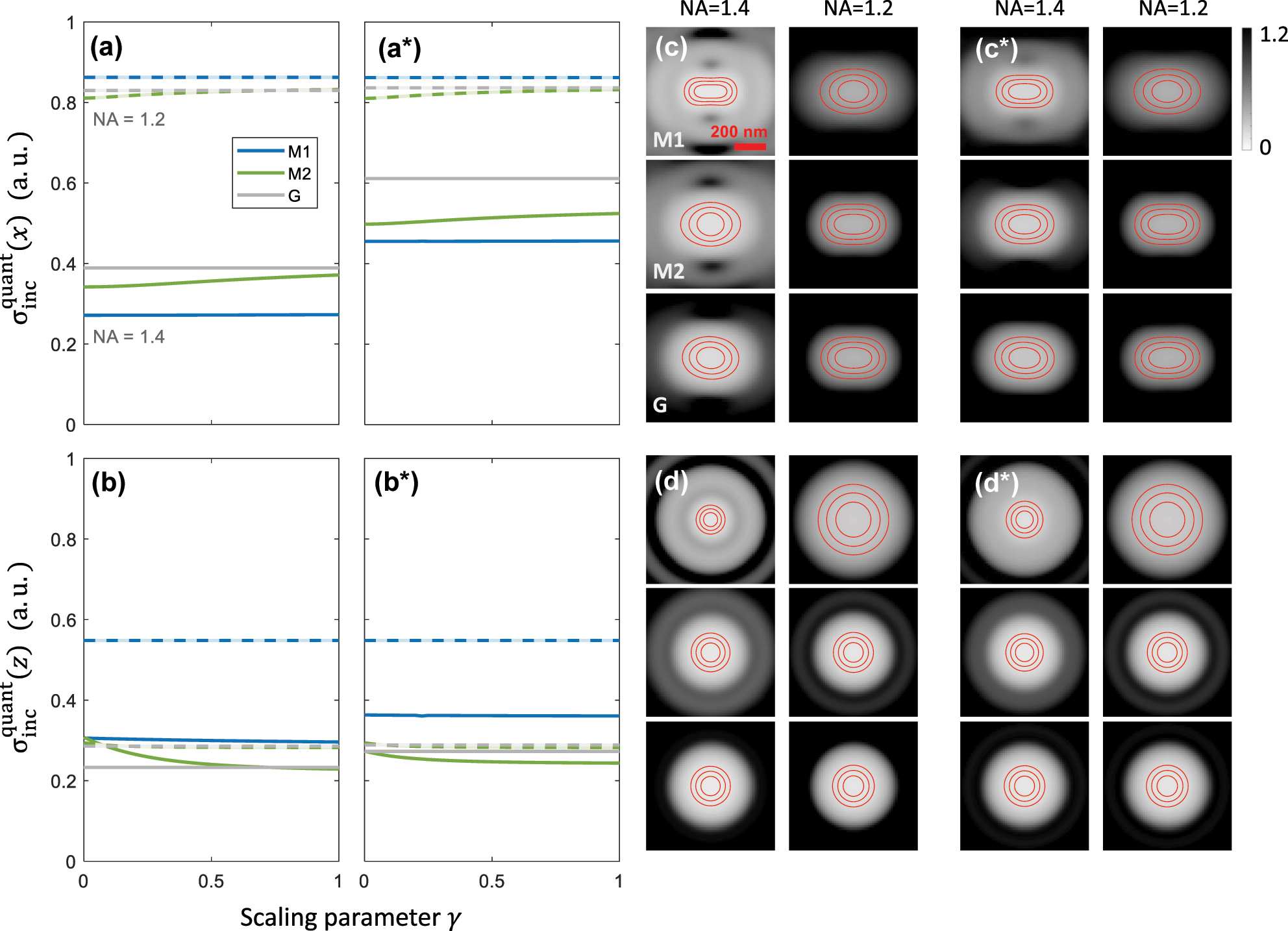
Dependence of quantum Cramér–Rao bound of Eq. (7) on the scaling parameter γ and the particle position
R
0. Panels (a, b) report the scaling parameter dependence of the bound
In Figure 7, we investigate the dependence of
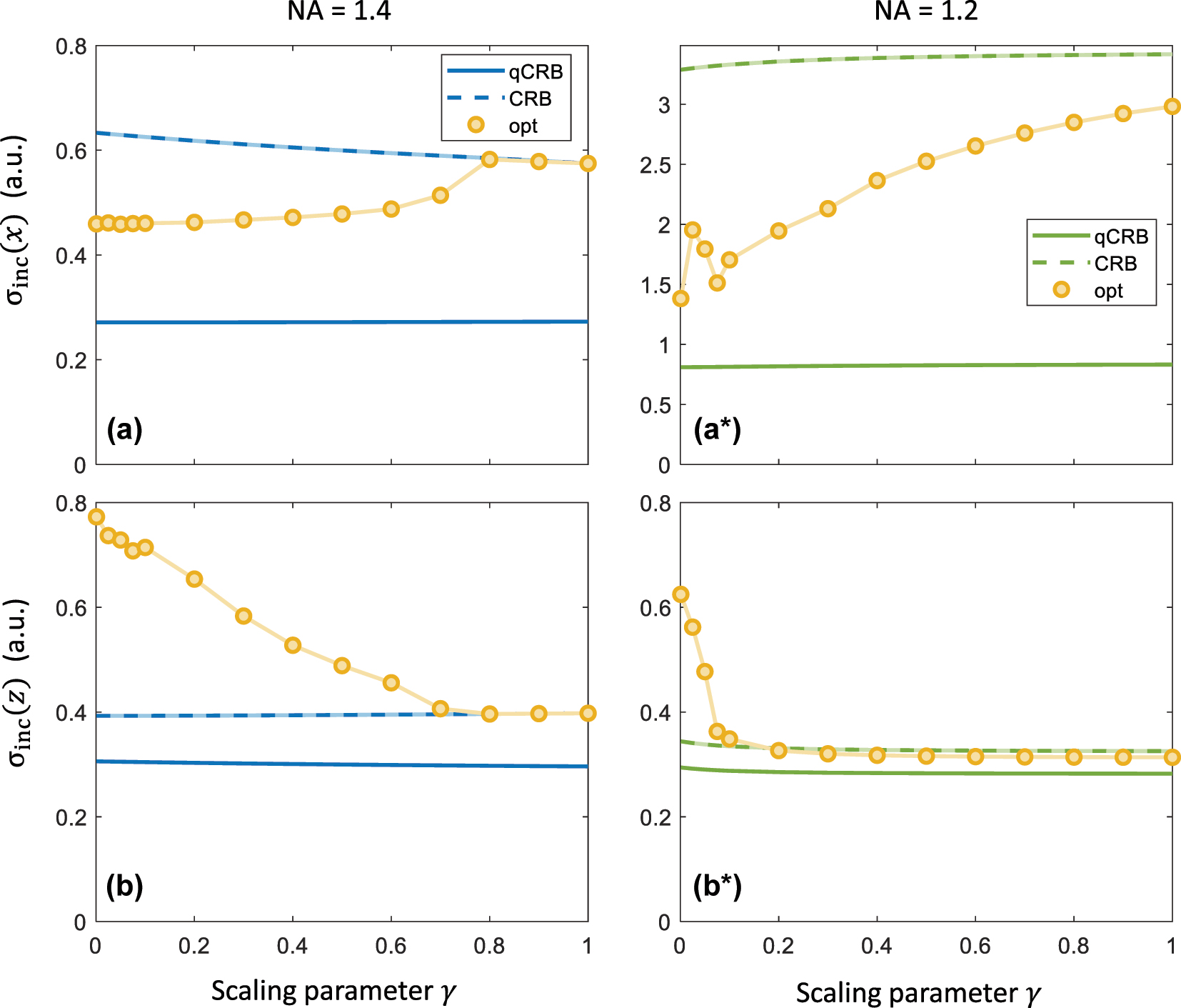
Dependence of quantum and iscat Cramér–Rao bound on the scaling parameter γ. Panels (a) and (b) show the dependence of the quantum (solid lines) and iscat (dashed lines) bounds for localization along x and z, respectively, and for NA = 1.4 and the mode M1 with radial polarization. The symbols report the bounds obtained from the optimization of the iscat Fisher information. (a*, b*) Same as (a, b) but for NA = 1.2.
References
[1] N. S. Ginsberg, C.-L. Hsieh, P. Kukura, M. Piliarik, and V. Sandoghdar, “Interferometric scattering microscopy,” Nat. Rev. Methods Primers, vol. 5, no. 1, p. 23, 2025, https://doi.org/10.1038/s43586-025-00391-1.Suche in Google Scholar
[2] B. E. Bouma et al.., “Optical coherence tomography,” Nat. Rev. Methods Primers, vol. 2, no. 1, p. 79, 2022, https://doi.org/10.1038/s43586-022-00162-2.Suche in Google Scholar PubMed PubMed Central
[3] T. Juffmann, S. Nimmrichter, F. Balzarotti, and J. Dong, “Quantum Fisher information in localization microscopy,” Photoniques, vol. 131, p. 58, 2025, https://doi.org/10.1051/photon/202513158.Suche in Google Scholar
[4] R. W. Taylor and V. Sandoghdar, “Interferometric scattering (iSCAT) microscopy and related techniques,” in Label-Free Super-Resolution Microscopy, V. Astratov, Ed., Cham, Springer International Publishing, 2019, pp. 25–65.10.1007/978-3-030-21722-8_2Suche in Google Scholar
[5] J. Icha, M. Weber, J. C. Waters, and C. Norden, “Phototoxicity in live fluorescence microscopy, and how to avoid it,” BioEssays, vol. 39, no. 8, p. 1700003, 2017, https://doi.org/10.1002/bies.201700003.Suche in Google Scholar PubMed
[6] K. McKenzie, M. Maclean, M. Helen Grant, P. Ramakrishnan, S. J. MacGregor, and J. G. Anderson, “The effects of 405 nm light on bacterial membrane integrity determined by salt and bile tolerance assays, leakage of UV-absorbing material and SYTOX green labelling,” Microbiology, vol. 162, no. 9, pp. 1680–1688, 2016, https://doi.org/10.1099/mic.0.000350.Suche in Google Scholar PubMed PubMed Central
[7] J. Chao, E. S. Ward, and R. J. Ober, “Fisher information theory for parameter estimation in single molecule microscopy: tutorial,” J. Opt. Soc. Am. A, vol. 33, no. 7, p. B36, 2016. https://doi.org/10.1364/josaa.33.000b36.Suche in Google Scholar
[8] M. Tsang, R. Nair, and X.-M. Lu, “Quantum theory of superresolution for two incoherent optical point sources,” Phys. Rev. X, vol. 6, no. 3, p. 031033, 2016. https://doi.org/10.1103/physrevx.6.031033.Suche in Google Scholar
[9] R. Nair and M. Tsang, “Interferometric superlocalization of two incoherent optical point sources,” Opt. Express, vol. 24, no. 4, pp. 3684–3701, 2016, https://doi.org/10.1364/oe.24.003684.Suche in Google Scholar PubMed
[10] M. Paúr, B. Stoklasa, Z. Hradil, L. L. Sánchez-Soto, and J. Rehacek, “Achieving the ultimate optical resolution,” Optica, vol. 3, no. 10, pp. 1144–1147, 2016, https://doi.org/10.1364/optica.3.001144.Suche in Google Scholar
[11] Z. Hradil, J. Řeháček, L. Sánchez-Soto, and B.-G. Englert, “Quantum Fisher information with coherence,” Optica, vol. 6, no. 11, pp. 1437–1440, 2019, https://doi.org/10.1364/optica.6.001437.Suche in Google Scholar
[12] D. Bouchet, J. Dong, D. Maestre, and T. Juffmann, “Fundamental bounds on the precision of classical phase microscopes,” Phys. Rev. Appl., vol. 15, no. 2, p. 024047, 2021, https://doi.org/10.1103/physrevapplied.15.024047.Suche in Google Scholar
[13] J. Dong, D. Maestre, C. Conrad-Billroth, and T. Juffmann, “Fundamental bounds on the precision of iSCAT, COBRI and dark-field microscopy for 3d localization and mass photometry,” J. Phys. D, vol. 54, no. 39, p. 394002, 2021. https://doi.org/10.1088/1361-6463/ac0f22.Suche in Google Scholar
[14] L. Kienesberger, T. Juffmann, and S. Nimmrichter, “Quantum limits of position and polarizability estimation in the optical near field,” Phys. Rev. Res., vol. 6, no. 2, p. 23204, 2024, https://doi.org/10.1103/physrevresearch.6.023204.Suche in Google Scholar
[15] N. J. Brooks, C.-C. Liu, Y.-H. Chen, and C.-L. Hsieh, “Point spread function engineering for spiral phase interferometric scattering microscopy enables robust 3D single-particle tracking and characterization,” ACS Photonics, vol. 11, no. 12, pp. 5239–5250, 2024, https://doi.org/10.1021/acsphotonics.4c01481.Suche in Google Scholar
[16] F. Müller, E. Köse, A. J. Meixner, E. Schäffer, and D. Braun, “Interferometric mass photometry at the quantum limit of sensitivity,” Phys. Rev. A, vol. 111, no. 4, p. 043501, 2025. https://doi.org/10.1103/physreva.111.043501.Suche in Google Scholar
[17] S. Koppell and M. Kasevich, “Information transfer as a framework for optimized phase imaging,” Optica, vol. 8, no. 4, pp. 493–501, 2021, https://doi.org/10.1364/optica.412129.Suche in Google Scholar
[18] C. Dwyer, “Quantum limits of transmission electron microscopy,” Phys. Rev. Lett., vol. 130, no. 5, p. 056101, 2023, https://doi.org/10.1103/physrevlett.130.056101.Suche in Google Scholar
[19] C. Dwyer and D. M. Paganin, “Quantum and classical Fisher information in four-dimensional scanning transmission electron microscopy,” Phys. Rev. B, vol. 110, no. 2, p. 024110, 2024, https://doi.org/10.1103/physrevb.110.024110.Suche in Google Scholar
[20] F. Balzarotti et al.., “Nanometer resolution imaging and tracking of fluorescent molecules with minimal photon fluxes,” Science, vol. 355, no. 6325, pp. 606–612, 2017, https://doi.org/10.1126/science.aak9913.Suche in Google Scholar PubMed
[21] Y. Liu, J. Dong, J. A. Maya, F. Balzarotti, and M. Unser, “Point-spread-function engineering in minflux: optimality of donut and half-moon excitation patterns,” Opt. Lett., vol. 50, no. 1, pp. 37–40, 2024, https://doi.org/10.1364/ol.543882.Suche in Google Scholar
[22] M. Rosati, M. Parisi, I. Gianani, M. Barbieri, and G. Cincotti, “Fundamental precision limits of fluorescence microscopy: a perspective on minflux,” Opt. Lett., vol. 49, no. 17, pp. 4938–4941, 2024, https://doi.org/10.1364/ol.530358.Suche in Google Scholar PubMed
[23] T. A. Hensel, J. O. Wirth, O. L. Schwarz, and S. W. Hell, “Diffraction minima resolve point scatterers at few hundredths of the wavelength,” Nat. Phys., vol. 21, pp. 412–420, 2024, https://doi.org/10.1038/s41567-024-02760-1.Suche in Google Scholar
[24] D. Bouchet, S. Rotter, and A. P. Mosk, “Maximum information states for coherent scattering measurements,” Nat. Phys., vol. 17, p. 564, 2021, https://doi.org/10.1038/s41567-020-01137-4.Suche in Google Scholar
[25] I. Starshynov et al.., “Model-free estimation of the Cramér–Rao bound for deep learning microscopy in complex media,” Nat. Photonics, vol. 19, no. 6, pp. 593–600, 2025, https://doi.org/10.1038/s41566-025-01657-6.Suche in Google Scholar
[26] L. M. Rachbauer, D. Bouchet, U. Leonhardt, and S. Rotter, “How to find optimal quantum states for optical micromanipulation and metrology in complex scattering problems: tutorial,” JOSA B, vol. 41, no. 9, pp. 2122–2139, 2024, https://doi.org/10.1364/josab.522649.Suche in Google Scholar
[27] J. Hüpfl et al.., “Continuity equation for the flow of Fisher information in wave scattering,” Nat. Phys., vol. 20, no. 8, pp. 1294–1299, 2024, https://doi.org/10.1038/s41567-024-02519-8.Suche in Google Scholar
[28] F. Hitzelhammer et al.., “Unified simulation platform for interference microscopy,” ACS Photonics, vol. 11, no. 7, p. 2745, 2024. https://doi.org/10.1021/acsphotonics.4c00621.Suche in Google Scholar PubMed PubMed Central
[29] J. S. Eismann and P. Banzer, “Sub-diffraction-limit Fourier-plane laser scanning microscopy,” Optica, vol. 9, no. 5, pp. 455–460, 2022, https://doi.org/10.1364/optica.450712.Suche in Google Scholar
[30] W. Kasprzycka, W. Szumigraj, P. Wachulak, and E. A. Trafny, “New approaches for low phototoxicity imaging of living cells and tissues,” BioEssays, vol. 46, no. 5, p. 2300122, 2024. https://doi.org/10.1002/bies.202300122.Suche in Google Scholar PubMed
[31] E. Bornstein, W. Hermans, S. Gridley, and J. Manni, “Near-infrared photoinactivation of bacteria and fungi at physiologic temperatures,” Photochem. Photobiol., vol. 85, no. 6, pp. 1364–1374, 2009. https://doi.org/10.1111/j.1751-1097.2009.00615.x.Suche in Google Scholar PubMed
[32] U. Hohenester, N. Reichelt, and G. Unger, “Nanophotonic resonance modes with the nanobem toolbox,” Comput. Phys. Commun., vol. 276, p. 108337, 2022, https://doi.org/10.1016/j.cpc.2022.108337.Suche in Google Scholar
[33] U. Hohenester, “Nanophotonic resonators in stratified media with the nanobem toolbox,” Comput. Phys. Commun., vol. 294, p. 108949, 2024, https://doi.org/10.1016/j.cpc.2023.108949.Suche in Google Scholar
[34] R. Gholami Mahmoodabadi et al.., “Point spread function in interferometric scattering microscopy (iSCAT). Part i: aberrations in defocusing and axial localization,” Opt. Express, vol. 28, no. 18, p. 25969, 2020. https://doi.org/10.1364/oe.401374.Suche in Google Scholar PubMed
[35] B. Richards and E. Wolf, “Electromagnetic simulation in optical systems II. Structure of the image field in an aplanatic system,” Proc. R. Soc. Lond. Ser. A, vol. 253, no. 1274, p. 358, 1959.10.1098/rspa.1959.0200Suche in Google Scholar
[36] U. Hohenester, Nano and Quantum Optics, Cham, Switzerland, Springer, 2020.10.1007/978-3-030-30504-8Suche in Google Scholar
[37] G. Young et al.., “Quantitative mass imaging of single biological macromolecules,” Science, vol. 360, no. 6387, pp. 423–427, 2018, https://doi.org/10.1126/science.aar5839.Suche in Google Scholar PubMed PubMed Central
[38] U. Hohenester, M. Simic, R. Hauer, L. Huber, and C. Hill, “Unified simulation platform for optical tweezers and optofluidic force induction,” ACS Photonics, vol. 12, no. 4, p. 2242, 2025. https://doi.org/10.1021/acsphotonics.5c00254.Suche in Google Scholar PubMed PubMed Central
[39] M. Weimar et al.., “Controlling the flow of information in optical metrology,” arXiv preprint, arXiv:2508.13640, 2025.Suche in Google Scholar
[40] F. Hitzelhammer, J. Dong, U. Hohenester, and T. Juffmann, “Fundamental bounds for off-axis illumination in interferometric and rotating coherent scattering microscopy,” arXiv preprint, arXiv:2510.03034, 2025.Suche in Google Scholar
© 2025 the author(s), published by De Gruyter, Berlin/Boston
This work is licensed under the Creative Commons Attribution 4.0 International License.