A new family of compound exponentiated logarithmic distributions with applications to lifetime data
-
Nooshin Hakamipour


Abstract
The logarithmic distribution and a given lifetime distribution are compounded to construct a new family of lifetime distributions. The compounding is performed with respect to maxima. Expressions are derived for lifetime properties like moments and the behavior of extreme values. Estimation procedures for the method of maximum likelihood are also derived and their performance assessed by a simulation study. Three real data (including two lifetime data) applications are described that show superior performance (assessed with respect to Kolmogorov Smirnov statistics, likelihood values, AIC values, BIC values, probability-probability plots and density plots) versus at least five known lifetime models, with each model having the same number of parameters as the model it is compared to.
1 Introduction
There exist numerous distributions for modeling lifetime data, however, some of these distributions lack motivation from a lifetime context. For example, there is no apparent physical motivation for the gamma distribution. It only has a more general mathematical form compared with the exponential distribution with one additional parameter, so it has nicer properties and provides better fits. The same arguments apply to many other distributions.
The aim of this note is to introduce a new family of distributions with sound physical motivation as in [23], [9] and [10]. As explained in subsequent sections, the proposed family encompasses the behavior of and provides better fits (assessed via a comparison of Kolmogorov Smirnov statistics, likelihood values, AIC values, BIC values, probability-probability plots and density plots) compared with several known lifetime distributions having the same number of parameters. We feel that this is a remarkable feature.
The motivation we provide for the new distribution is based on failures of a system. Here, the words “failures” and “system” should not be interpreted as relating purely to an electronic or a mechanical system, but instead in a more general sense.
Suppose a system has N entities operating independently and identically in parallel, where N is a logarithmic random variable with the PMF:
where 0 < p < 1. A logarithmic distribution for the number entities in a system is not unreasonable. [29], [30] used a logarithmic distribution to characterize the abundance of species of animals or plants. [24] supposed that the number of demands in a batch follows the logarithmic distribution. [4] modeled the number of eggs in a cluster by the logarithmic distribution.
Suppose each entity has α sub-entities operating independently and identically in parallel, where α is an integer. Assume that the lifetimes of the sub-entities are independent of N and have the common PDF g (⋅) and the common CDF G (⋅). Then the lifetime of the system, say X, has the CDF
The corresponding PDF is:
The corresponding HRF is:
The corresponding quantile function is
where G−1(⋅) denotes the inverse function of G (⋅). Here, α and p are shape parameters. For continuity and simplicity, we shall assume hereafter that α can take any positive real value and not just integers (similar to approximating a discrete distribution by a continuous one).
We shall refer to the distribution given by (1) and (2) as the Compound Exponentiated Logarithmic (CEL) distribution. The construction of this distribution is fundamentally different from those of several recently proposed distributions, see [27], [2] and [14]. These papers consider X = min (X1, X2, … , XN) with the Xi assumed to come from either an exponential or a Weibull distribution. That is, they apply to series systems and the choice for the distribution of Xi is restricted. Here, we impose no such restrictions. [13] consider distributions of U = min (X1, X2, … , XN) and V = max (X1, X2, … , XN) with N assumed to be a geometric random variable. However, geometric random variables are “time to event” variables and it makes little sense to model the number of entities in a system by a geometric distribution. In any case, [13] provide no motivation for choosing N to be a geometric random variable. Furthermore, [13] derive properties of U and V only for the particular cases that Xi is an exponential or a Weibull random variable.
The situation giving rise to (1) can encompass a wide range of examples. Here, we discuss just one example. Suppose that N storms are observed in one year. The word “storm” could mean a sequence of days experiencing rainfall, a sequence of days experiencing snowfall, etc. Suppose each storm has a fixed duration, α. This is not an unreasonable assumption if storm durations are not too variable (in which case zeros can be added to make the durations equal). Suppose also that N is a logarithmic random variable and let G (⋅) denote the CDF of daily rainfall, CDF of daily snowfall, etc. Then X will represent the annual maximum rainfall, annual maximum snowfall, etc.
The aim of this note is to study the mathematical properties of the CEL distribution and to illustrate its applicability. The contents are organized as follows. In Section 2, we derive general mathematical properties of the CEL distribution. These include expansions for the PDF and the CDF, shape properties of (2) and (3), moments, moment generating function, characteristic function, and asymptotic distributions of the extreme order statistics. All of these properties are clearly relevant for a random variable representing lifetime. Other properties like mean deviations and entropies can also be derived, but they take complicated forms. The maximum likelihood estimation is considered in Section 3. Section 4 gives applications using three real data sets. Finally, some conclusions are noted in Section 5.
Throughout this note, we shall focus attention on a particular CEL distribution by taking the baseline CDF G to correspond to an exponential distribution with scale parameter β. The rationale for this choice is that the exponential distribution is the first and the most widely used model for failure times. Then (2) becomes
for x > 0, α > 0, β > 0, and 0 < p < 1. The corresponding HRF is
for x > 0, α > 0, β > 0, and 0 < p < 1. We shall refer to (4) as the Generalized Exponential Logarithmic (GEL) PDF. The limiting case of (4) for p ↑ 1 is the exponentiated exponential distribution due to [6]. The limiting case of (4) for p ↑ 1 and α = 1 is the exponential distribution.
We shall see later in Section 4 that the GEL distribution performs well with respect to at least five known models in spite of being the simplest member of the class of CEL distributions. (The GEL distribution corresponds to the failure times following the exponential distribution, the simplest possible model.) Hence, other members of the class of CEL distributions can only be expected to perform better than the GEL distribution. Hence, we feel no need to consider more than one particular case of the class of CEL distributions.
2 Mathematical properties
Section 2.1 shows how fX (⋅) and FX (⋅) can be expanded in terms of g (⋅) and G (⋅). These expansions are useful technical tools for later use. Section 2.2 derives shape characteristics of fX (⋅) and hX (⋅) in terms of g (⋅) and G (⋅). For a given CEL distribution, these characteristics can be used to determine possible shapes of the PDF or the HRF of X. Section 2.3 derives moment properties of X. These can be useful for calculating basic measures like the mean, variance, coefficient of variation, skewness and kurtosis. Moment properties can also be used for estimation. Section 2.4 expresses the extreme value behavior of X in terms of that of a random variable specified by g (⋅) and G (⋅). This can be useful in determining the extreme domains of attraction of a given CEL distribution.
2.1 Expansions for PDF and CDF
Some useful expansions for (1) and (2) can be derived using the concept of exponentiated distributions. A random variable is said to have the exponentiated-G distribution with parameter a > 0, if its PDF and CDF are
and
respectively. Many authors have studied exponentiated distributions. These include among others [15], [5], [6], [18], [11] and [20].
We now provide expansions for (1) and (2), each in terms of (6) and (7). Expanding the logarithmic term in (1), we can write (1) and (2) as
and
respectively. So, several properties of the CEL distribution can be obtained by knowing those of exponentiated distributions ([16], [6], [21]).
2.2 Asymptotes and shapes
The asymptotes of (1), (2), and (3) as x → 0, ∞ are given by
Note that the right hand sides of (10) and (12) are decreasing functions of p. The right hand sides of (11), (13) and (14) are increasing functions of p. It follows from (11) that fX (⋅) behaves like g (⋅) for very large x. Also, hX (⋅) behaves like the HRF corresponding to g (⋅) for very large x.
An analytical description of the shapes of (2) and (3) is possible. The critical points of the PDF are the roots of the equation:
(16) may have one or more roots. If x = x0 is a root of (16), then it corresponds to a local maximum, a local minimum or a point of inflexion depending on whether λ (x0) < 0, λ (x0) > 0 or λ (x0) = 0, where
The critical points of the HRF are the roots of:
(17) may have one or more roots. If x = x0 is a root of (17), then it corresponds to a local maximum, a local minimum or a point of inflexion depending on whether λ (x0) < 0, λ (x0) > 0 or λ (x0) = 0, where
It follows from (16) that ∂ log fX(x)/∂ x is an increasing function of p with
and
It follows from (17) that ∂ log hX(x)/∂ x is a decreasing function of p with
and
Calculations using (10)–(15) show that the upper tail of (4) decays exponentially and that the lower tail of (4) decays polynomially. Both the upper and lower tails of (5) approach some constants. In fact, hX (0) = −α λ (1 − p)/ log p and hX (∞) = λ.
Calculations using (16) show that (4) can be either monotonically decreasing or unimodal. Calculations using (17) show that (5) can be either monotonically decreasing, monotonically increasing or upside down bathtub shaped. The exponentiated exponential distribution (the limiting case of the GEL distribution for p ↑ 1) cannot exhibit upside down bathtub shaped hazard rates.
Upside down bathtub hazard rates are common in reliability and survival analysis. For example, such hazard rates can be observed in the course of a disease whose mortality reaches a peak after some finite period and then declines gradually [25]. For other practical examples yielding upside down bathtub hazard rates, see [26].
2.3 Moment properties
Let (1) denote the CDF of a random variable X. Let ha (⋅) and Ha (⋅) denote, respectively, the PDF and CDF of a random variable Za. Then, using the expansions, (8) and (9), we have
Similarly, the moment generating function and the characteristic function of X can be expressed as
and
respectively, where
The moments, moment generating function and the characteristic function of the GEL distribution follow immediately from (18)–(20) and the moments, moment generating function and characteristic function of the exponentiated exponential distribution. The latter are given explicitly in [19: Section 2]: if Z is an exponentiated exponential random variable with shape parameter α and scale parameter λ, then
and
where
2.4 Extreme values
If X = (X1 + ⋯ + Xn) /n denotes the mean of a random sample from (2), then by the central limit theorem
Suppose firstly that the Gumbel distribution is the max domain of attraction of G. By [12: Chapter 1], there must exist a strictly positive function, say h(t), such that
But, using (13), we note that
So, the Gumbel distribution is also the max domain of attraction of FX with
for some suitable norming constants an > 0 and bn.
Suppose secondly that the Fréchet distribution is the max domain of attraction of G. By [12: Chapter 1], there must exist a β < 0 such that
But, using (13), we note that
So, the Fréchet distribution is also the max domain of attraction of FX with
for some suitable norming constants an > 0 and bn.
Suppose thirdly that the Weibull distribution is the max domain of attraction of G. By [?: ]hapter 1letal1987, there must exist a c > 0 such that
for every x < 0. But, using (12), we note that
So, the Weibull distribution is also the max domain of attraction of FX with
for some suitable norming constants an > 0 and bn.
The same argument applies to min domains of attraction. That is, G and FX have the same min domain of attraction.
Since the exponential distribution belongs to the max (min) domain of attraction of the Gumbel (Weibull) distribution, we have that the max (min) domain of attraction of the GEL distribution is the Gumbel (Weibull) distribution.
3 Estimation
Section 3.1 estimates the parameters of the CEL distribution by the method of maximum likelihood. It also derives the associated observed information matrix. Section 3.2 assesses the performance of the maximum likelihood estimates with respect to biases and mean squared errors. For this assessment, we consider the GEL distribution, the simplest possible member of the class of CEL distributions.
3.1 Maximum likelihood estimation
Let x1, x2, …, xn be a random sample from (2). Let Θ denote a q-dimensional vector containing the parameters in G (⋅). Then the log-likelihood function, log L = log L (p, α, Θ), is
The first derivatives of log L with respect to p, α and Θ are:
The maximum likelihood estimates of (p, α, Θ), say (p͡, α͡, Θ͡), are the simultaneous solutions of the equations ∂ log L/∂ p = 0, ∂ log L/∂ α = 0 and ∂ log L/∂ Θ = 0.
Maximization of (21) can be performed by using well established routines like nlminb or optim in the R statistical package [22]. Our numerical calculations showed that the surface of (21) was smooth for given smooth functions g (⋅) and G (⋅). The routines were able to locate the maximum of the likelihood surface for a wide range of smooth functions and for a wide range of starting values. However, to ease the computations it is useful to have reasonable starting values. These can be obtained, for example, by equating the sample and theoretical quantiles. For r = 1, … , q + 2, let qr denote the sample quantile corresponding to the probability r/(q + 3). Equating these quantiles with the theoretical versions given in Section 1, we have
These equations can be solved simultaneously to obtain the initial estimates.
For interval estimation of (p, α, Θ) and tests of hypothesis, one requires the Fisher information matrix. We can express the observed Fisher information matrix of (p͡, α͡, Θ͡) as
where
For large n, the distribution of
It is reasonable to ask: how large should n be for the normal approximation to hold? This question is answered in the next section.
3.2 A simulation study
In this section, we assess the performance of the maximum likelihood estimates given by\linebreak (22)–(24) with respect to the sample size n for the GEL distribution. The assessment of the performance of the maximum likelihood estimates of (α, β, p) is based on a simulation study:
generate ten thousand samples of size n from (4). The inversion method was used to generate samples, i.e., variates of the GEL distribution were generated using
where U ∼ U(0, 1) is a uniform variate on the unit interval;
compute the maximum likelihood estimates for the ten thousand samples, say α͡i, β͡i and p͡i for i = 1, 2, … , 10000;
compute the biases and mean squared errors given by
for e = α, β, p.
We repeated these steps for n = 10, 20, … , 500 with α = 2, β = 2 and p = 0.5, so computing biasα (n), biasβ (n), biasp (n), MSEα (n), MSEβ (n) and MSEp (n) for n = 10, 20, … , 500.
Figures 1 and 2 show how the biases and the mean squared errors vary with respect to n. The broken line in Figure 1 corresponds to the biases being zero. The broken line in Figure 2 corresponds to the mean squared errors being zero.
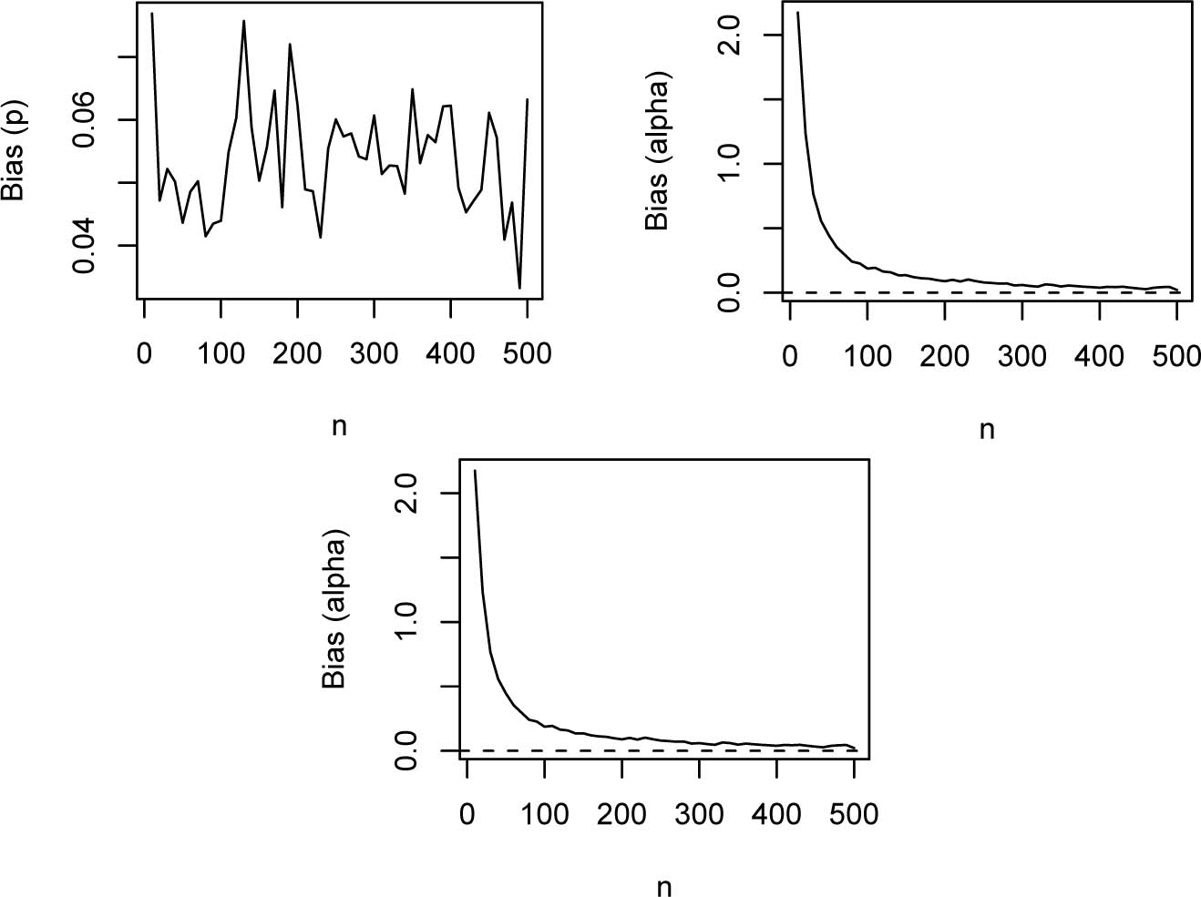
Biases of α͡, β͡ and p͡ versus n = 10, 20, … , 500.
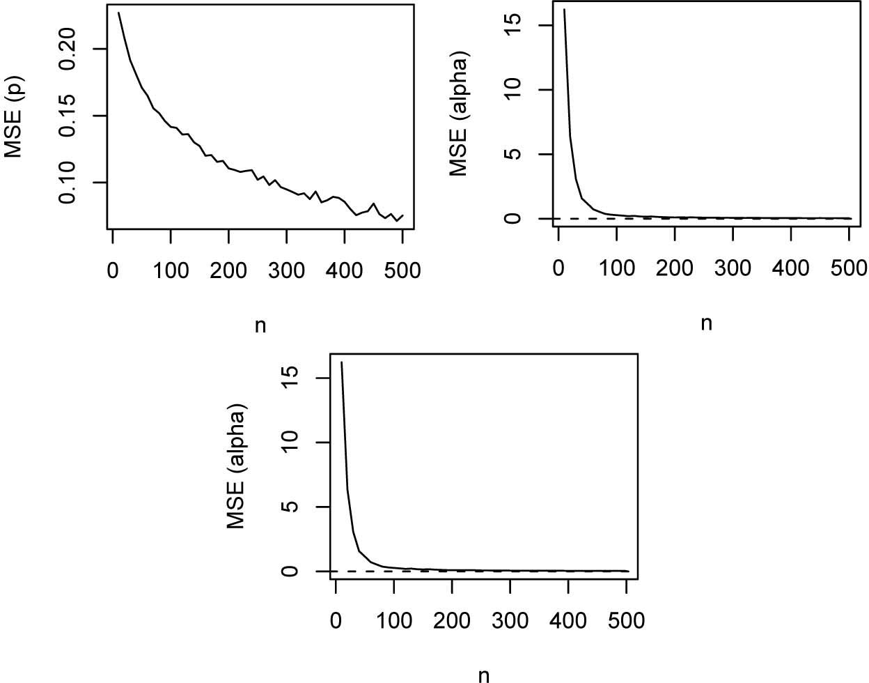
Mean squared errors of α͡, β͡ and p͡ versus n = 10, 20, … , 500.
The following observations can be made:
the biases generally appear positive for each parameter;
the magnitude of the biases generally decreases to zero as n → ∞;
the biases appear smallest for p;
the biases appear largest for α;
the mean squared errors generally decrease to zero as n → ∞;
the mean squared errors appear smallest for p;
the mean squared errors appear largest for α;
the convergence of the biases to zero appears slowest for p with convergence still not reached for n as large as five hundred;
the convergence of the biases to zero appears fastest for α;
the convergence of the mean squared errors to zero appears slowest for p with convergence still not reached for n as large as five hundred;
the convergence of the mean squared errors to zero appears fastest for α.
For brevity, we have presented results only for α = 2, β = 2 and p = 0.5, however, the results were similar for other choices for α, β and p.
4 Applications
In this section, we fit the GEL distribution to three real data sets. The first data set consists of waiting times in minutes of one hundred bank customers [3]. The second data set consists of active repair times in hours (see page 156 of [28]). The third data set consists of March precipitation for Minneapolis Saint Paul [8].
We compare the fit of the GEL distribution in (4) with five alternative models each containing three parameters: the generalized exponential-Poisson (GEP) distribution (see [1]) with PDF:
the exponential Weibull (EW) distribution (see [16, 17]) with PDF:
the Weibull Poisson (WP) distribution [7] with PDF
the generalized exponential (GE) distribution [6] with PDF:
the generalized exponential geometric (GEG) distribution [25] with PDF:
The maximum likelihood estimates, corresponding standard errors, the log-likelihood values, the Kolmogorov Smirnov statistics, associated p-values, the AIC values and the BIC values are shown in Tables 1 to 3. The standard errors were computed by inverting the observed information matrices, see Section 3.1. We can see that the largest log-likelihood value, the largest p-value, the smallest AIC value and the smallest BIC value are obtained for the GEL distribution. The results show that the GEL distribution yields the best fits.
Parameter estimates and associated values for the first data set.
| Distribution | Estimates (standard errors) | Log-likelihood | K-S | p-value | AIC | BIC |
|---|---|---|---|---|---|---|
| GEL | (2.3266, 0.1478, 0.5671) (2.1942, 0.1069, 0.4053) | −317.0107 | 0.0761 | 0.7141 | 640.0214 | 647.8369 |
| WP | (0.0596, 1.7228, 2.9720) (0.0158, 1.6526, 0.8982) | −318.3816 | 0.0821 | 0.4847 | 642.7631 | 650.5787 |
| EW | (2.5729, 0.9060, 0.1904) (1.3821, 0.5958, 0.1671) | −317.1054 | 0.0858 | 0.5690 | 640.2108 | 648.0263 |
| GEP | (2.7193, 0.1593, 0.7999) (0.9171, 0.1387, 0.0325) | −317.5271 | 0.1145 | 0.2271 | 641.0542 | 648.8697 |
| GE | (1.8929, 7.6563, 0.3460) (1.3703, 1.6305, 0.0237) | −318.8549 | 0.1077 | 0.1828 | 643.7097 | 651.5252 |
| GEG | (3.2316, 0.1397, 0.4231) (1.4594, 0.1258, 0.0531) | −318.0609 | 0.0776 | 0.5572 | 642.1218 | 649.9373 |
Parameter estimates and associated values for the second data set.
| Distribution | Estimates (standard errors) | Log-likelihood | K-S | p-value | AIC | BIC |
|---|---|---|---|---|---|---|
| GEL | (1.5085, 0.2040, 0.0700) (1.0042, 0.1718, 0.0544) | −102.7108 | 0.1195 | 0.7582 | 211.4217 | 216.9721 |
| WP | (0.1168, 1.0968, 3.5363) (0.1036, 0.9061, 2.3973) | −103.7616 | 0.1497 | 0.4878 | 213.5232 | 219.0736 |
| EW | (2.9085, 0.5779, 1.2000) (1.6546, 0.3251, 0.2387) | −103.2490 | 0.1883 | 0.2251 | 212.4979 | 218.0484 |
| GEP | (1.1434, 0.2119, 0.1000) (1.0036, 0.0798, 0.0828) | −109.5163 | 0.1439 | 0.5383 | 225.0326 | 230.5830 |
| GE | (0.2636, 47.0700, 0.2000) (0.1793, 10.0844, 0.0135) | −110.7692 | 0.2828 | 0.0152 | 227.5383 | 233.0887 |
| GEG | (9.7999, 0.0950, 0.9810) (0.1225, 0.0768, 0.7290) | −103.5101 | 0.1205 | 0.7493 | 213.0202 | 218.5706 |
Parameter estimates and associated values for the third data set.
| Distribution | Estimates (standard errors) | Log-likelihood | K-S | p-value | AIC | BIC |
|---|---|---|---|---|---|---|
| GEL | (3.6258, 1.0771, 0.5333) (2.6047, 0.0934, 0.0535) | −38.1570 | 0.0846 | 0.9744 | 82.3139 | 86.5175 |
| WP | (0.3990, 2.5829, 2.9895) (0.1012, 1.8698, 1.4216) | −39.8804 | 0.1231 | 0.7257 | 85.7609 | 89.9645 |
| EW | (2.8421, 1.0931, 1.2956) (1.1871, 1.0023, 0.2747) | −40.4429 | 0.2060 | 0.1479 | 88.3301 | 92.5337 |
| GEP | (3.7942, 1.3426, 0.3050) (1.4932, 1.0194, 0.1686) | −39.2024 | 0.1721 | 0.3193 | 84.4048 | 88.6084 |
| GE | (2.4402, 0.9992, −0.2501) (1.9948, 0.9868, 0.0932) | −39.1574 | 0.1243 | 0.7152 | 84.3149 | 88.5184 |
| GEG | (4.0001, 1.1323, 0.4223) (3.1755, 0.4400, 0.3087) | −39.0193 | 0.1624 | 0.3874 | 84.0386 | 88.2422 |
It is pleasing that the standard errors are less than the parameter estimates for each fitted distribution. It is also pleasing that the p-values based on Kolmogorov Smirnov statistics suggest that each fitted distribution adequately describes the data.
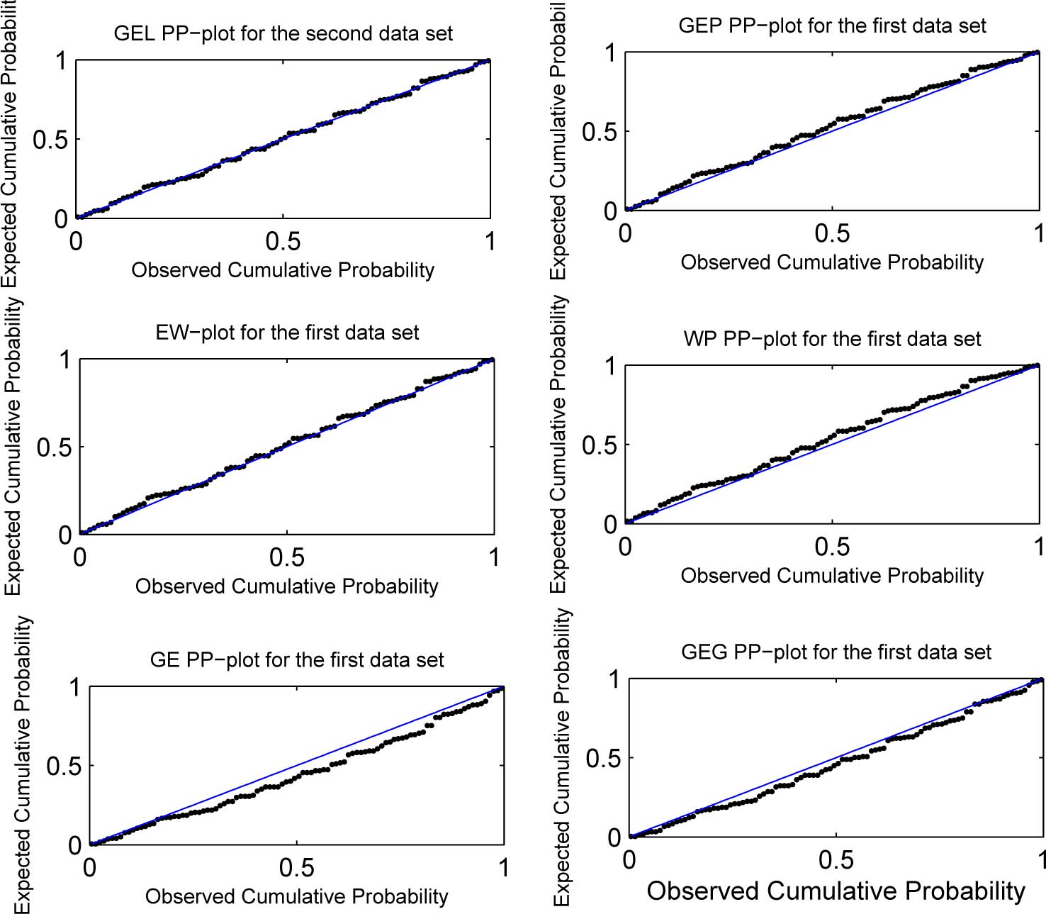
The probability-probability plots for the six fitted models and for each data set are shown in Figures 3 to 5. We can see that the GEL distribution has the points closest to the diagonal line for each data set.

Probability-probability plots for the fitted models for the first data set.
Probability-probability plots for the fitted models for the second data set.
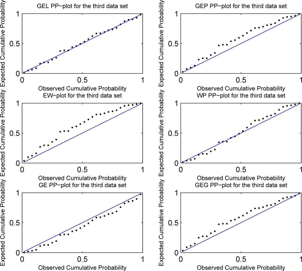
Probability-probability plots for the fitted models for the third data set.
A density plot compares the fitted PDFs of the models with the empirical histogram of the observed data. The density plots for the three data sets are shown in Figures 6 to 8. Again the fitted PDFs for the GEL distribution appear to capture the general pattern of the empirical histograms best.
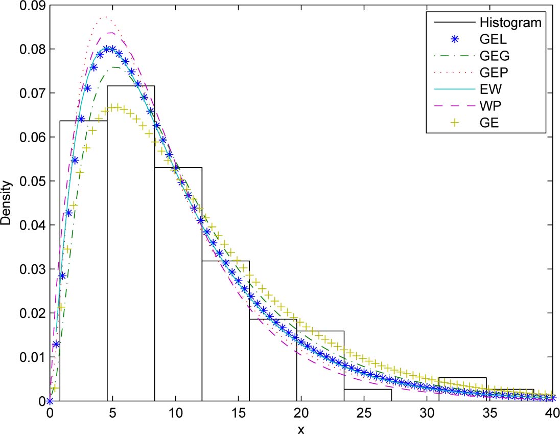
Fitted PDFs and the observed histogram for the first data set.
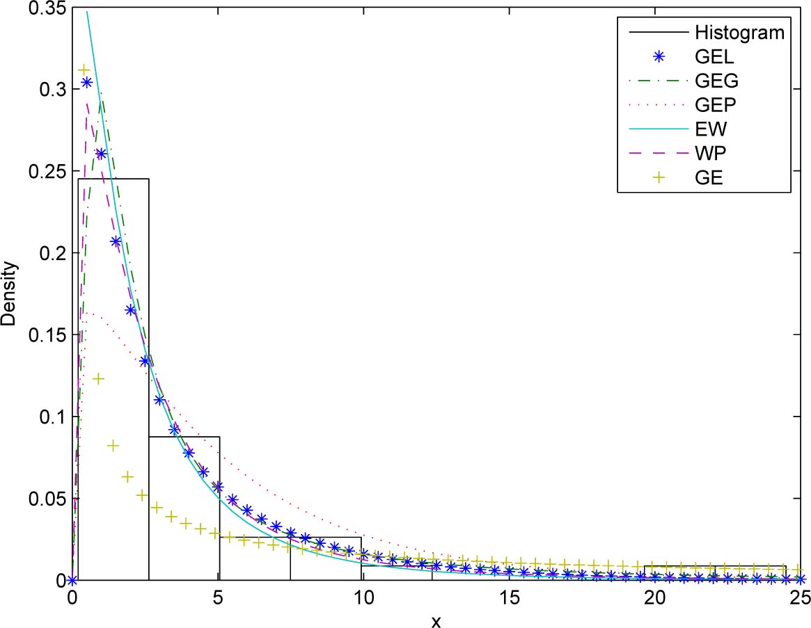
Fitted PDFs and the observed histogram for the second data set.
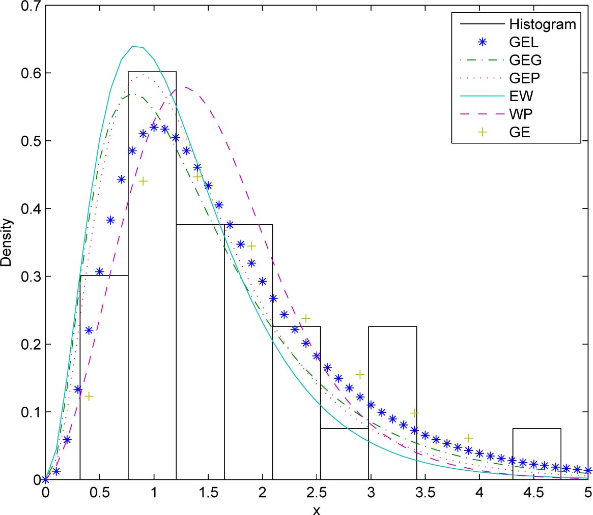
Fitted PDFs and the observed histogram for the third data set.
5 Conclusions
We have proposed a class of distributions by compounding the logarithmic distribution with any lifetime distribution. We have derived some mathematical properties of the class including shape properties, moment properties and the asymptotic distributions of the extreme order statistics. We have also discussed maximum likelihood estimation for the class of distributions and performed a simulation study to assess the performance of the maximum likelihood estimates.
The flexibility of the class is illustrated by fitting the generalized exponential logarithmic distribution, a particular member of the class, to three real data sets. We have compared the fit of the generalized exponential logarithmic distribution with five other distributions each having the same number of parameters. Evidence based on Kolmogorov Smirnov statistics, likelihood values, AIC values, BIC values, probability-probability plots and density plots shows that the generalized exponential logarithmic distribution outperforms all of the other distributions.
The Compound Exponentiated Logarithmic distribution in (1) and (2) is defined in terms of a random variable of the form max (Y1, Y2, … , YN). In classical insurance mathematics, the distribution of max (Y1, Y2, … , YN) is compared with the distribution of Y1 + Y2 + ⋯ + YN and this leads to the notion of subexponentiality. A future work is to see if subexponentiality has connections to the Compound Exponentiated Logarithmic distribution.
(Communicated by Gejza Wimmer )
References
[1] Barreto-Souza, W.—Cribari-Neto, F.: A generalization of the exponential-Poisson distribution, Stat. Probab. Lett. 79 (2009), 2493–2500.10.1016/j.spl.2009.09.003Search in Google Scholar
[2] Chahkandi, M.—Ganjali, M.: On some lifetime distributions with decreasing failure rate, Comput. Stat. Data Anal. 53 (2009), 4433–4440.10.1016/j.csda.2009.06.016Search in Google Scholar
[3] Ghitany, M. E.—Al-Mutairi, D. K.—Nadarajah, S.: Lindley distribution and its application, Math. Comput. Simulation 78 (2008), 493–506.10.1016/j.matcom.2007.06.007Search in Google Scholar
[4] Green, R. F.: Does aggregation prevent competitive exclusion? A response to Atkinson and Shorrocks, The American Naturalist 128 (1986), 301–304.10.1086/284562Search in Google Scholar
[5] Gupta, R. C.—Gupta, P. L.—Gupta, R. D.: Modeling failure time data by Lehman alternatives, Comm. Statist. Theory Methods 27 (1998), 887–904.10.1080/03610929808832134Search in Google Scholar
[6] Gupta, R. D.—Kundu, D.: Generalized exponential distributions, Aust. N. Z. J. Stat. 41 (1999), 173–188.10.1111/1467-842X.00072Search in Google Scholar
[7] Hemmati, F.—Khorram, E.—Rezakhah, S.: A new three parameter ageing distribution, J. Statist. Plann. Inference 141 (2011), 2266–2275.10.1016/j.jspi.2011.01.007Search in Google Scholar
[8] Hinkley, D.: On quick choice of power transformations, Amer. Statist. 26 (1977), 67–69.10.2307/2346869Search in Google Scholar
[9] Hussain, M. A.—Tahir, M. H.—Cordeiro, G. M.: A new Kumaraswamy generalized family of distributions: Properties and applications, Math. Slovaca 70 (2020), 1491–1510.10.1515/ms-2017-0429Search in Google Scholar
[10] Jamal, F.—Chesneau, C.—Nasir, M. A.—Saboor, A.—Altun, E.—Khan, M. A.: Math. Slovaca 70 (2020), 193–212.10.1515/ms-2017-0344Search in Google Scholar
[11] Kakde, C. S.—Shirke, D. T.: On exponentiated lognormal distribution, Int. J. Agric. Stat. 2 (2006), 319–326.Search in Google Scholar
[12] Leadbetter, M. R.—Lindgren, G.—Rootzén, H.: Extremes and Related Properties of Random Sequences and Processes, Springer Verlag, New York, 1987.Search in Google Scholar
[13] Marshall, A. W.—Olkin, I.: A new method for adding a parameter to a family of distributions with application to the exponential and Weibull families, Biometrika 84 (1997), 641–652.10.1093/biomet/84.3.641Search in Google Scholar
[14] Morais, A. L.—Barreto-Souza, W.: A compound class of Weibull and power series distributions, Comput. Stat. Data Anal. 55 (2011), 1410–1425.10.1016/j.csda.2010.09.030Search in Google Scholar
[15] Mudholkar, G. S.—Srivastava, D. K.: Exponentiated Weibull family for analyzing bathtub failure-rate data, IEEE Transactions on Reliability 42 (1993), 299–302.10.1109/24.229504Search in Google Scholar
[16] Mudholkar, G. S.—Srivastava, D. K.—Friemer, M.: The exponential Weibull family: analysis of the bus-motor-failure data, Technometrics 37 (1995), 436–445.10.1080/00401706.1995.10484376Search in Google Scholar
[17] Mudholkar, G. S.—Srivastava, D. K.—Kollia, G. D.: A generalization of the Weibull distribution with application to the analysis of survival data, J. Amer. Statist. Assoc. 91 (1996), 1575–1583.10.1080/01621459.1996.10476725Search in Google Scholar
[18] Nadarajah, S.: The exponentiated Gumbel distribution with climate application, Environmetrics 17 (2005), 13–23.10.1002/env.739Search in Google Scholar
[19] Nadarajah, S.: The exponentiated exponential distribution: A survey, AStA Advances in Statistical Analysis 95 (2011), 219–251.10.1007/s10182-011-0154-5Search in Google Scholar
[20] Nadarajah, S.—Gupta, A. K.: The exponentiated gamma distribution with application to drought data, Calcutta Stat. Assoc. Bull. 59 (2007), 29–54.10.1177/0008068320070103Search in Google Scholar
[21] Nadarajah, S.—Kotz, S.: The exponentiated type distributions, Acta Appl. Math. 92 (2006), 97–111.10.1007/s10440-006-9055-0Search in Google Scholar
[22] R Development Core Team: R: A Language and Environment for Statistical Computing. R Foundation for Statistical Computing, Vienna, Austria, 2018.Search in Google Scholar
[23] Saboor, A.—Khan, M. N.—Cordeiro, G. M.—Elbatal, I.—Pescim, R. R.: The beta exponentiated Nadarajah-Haghighi distribution: Theory, regression model and application, Math. Slovaca 69 (2019), 939–952.10.1515/ms-2017-0279Search in Google Scholar
[24] Sherbrooke, C. C.: Metric: A multi-echelon technique for recoverable item control, Oper. Res 16 (1968), 122–141.10.1287/opre.16.1.122Search in Google Scholar
[25] Silva, R. B.—Barreto-Souza, W.—Cordeiro, G. M.: A new distribution with decreasing, increasing and upside-down bathtub failure rate, Comput. Stat. Data Anal. 54 (2010), 935–944.10.1016/j.csda.2009.10.006Search in Google Scholar
[26] Singh, H.—Misra, N.: On redundancy allocations in systems, J. Appl. Probab. 31 (1994), 1004–1014.10.2307/3215324Search in Google Scholar
[27] Tahmasbi, R.—Rezaei, S.: A two-parameter lifetime distribution with decreasing failure rate, Comput. Stat. Data Anal. 52 (2008), 3889–3901.10.1016/j.csda.2007.12.002Search in Google Scholar
[28] von Alven, W. H.: Reliability Engineering, Prentice-Hall, New Jersey, 1964.Search in Google Scholar
[29] Williams, C. B.: The logarithmic series and its application to biological problems, Journal of Ecology 34 (1947), 253–272.10.2307/2256719Search in Google Scholar
[30] Williams, C. B.: The application of the logarithmic series to the frequency of occurrence of plant species in quadrats, Journal of Ecology 38 (1950), 107–138.10.2307/2256527Search in Google Scholar
© 2022 Mathematical Institute Slovak Academy of Sciences
This work is licensed under the Creative Commons Attribution 4.0 International License.
Articles in the same Issue
- Regular Papers
- Generalized hyperharmonic number sums with reciprocal binomial coefficients
- Gini index on generalized r-partitions
- Multiplicative functions of special type on Piatetski-Shapiro sequences
- Strengthenings of Young-type inequalities and the arithmetic geometric mean inequality
- Generalizations of the steffensen integral inequality for pseudo-integrals
- Subordination-implication problems concerning the nephroid starlikeness of analytic functions
- Boundedness and almost periodicity of solutions of linear differential systems
- On variational approaches for fractional differential equations
- Approximity of asymmetric metric spaces
- Approximation theorems for the new construction of Balázs operators and its applications
- On η-biharmonic hypersurfaces in pseudo-Riemannian space forms
- Chen’s first inequality for hemi-slant warped products in nearly trans-Sasakian manifolds
- Induced mappings on symmetric products of Hausdorff spaces
- The Teissier-G family of distributions: Properties and applications
- A new extension of the beta generator of distributions
- A new family of compound exponentiated logarithmic distributions with applications to lifetime data
- On two correlated linear models with common and different parameters
- On some applications of Duhamel operators