High resolution – large field-of-view 3D imaging of fiber-reinforced composites with complex microstructure: stitching of lab-CT scans with single fiber resolution

1 Introduction

3D material characterization has been on the rise since the 2000s, as it provides insight into the microstructure of materials. In particular, 3D X-ray computed tomography (CT) provides a relatively fast and readily available insight [1]. For example geometric models can be derived from 3D scans and used for simulation [2] or non-destructive testing for defects [3]. High resolution down to nm voxel size [4] and the possibility of quantitative in situ imaging [5] or other quantitative measurements [6] extend the range of applications in materials science. Especially for fiber reinforced polymers (FRP), such microscopic information can be used to better understand how its base materials, such as fibers and polymeric matrix or its processing process will affect the finished part. A major challenge in CT imaging of Carbon-FRPs is the hierarchical microstructure, with important structural details on length scales ranging from the size of individual fibers (approx. 1, …, 10 µm) to the arrangement of fibers in layers or bundles (100, …, 250 µm) to the size of the component (10, …, 100 mm), together with the low absorption contrast between the carbon fiber and the carbon-based polymer matrix. To overcome the latter and to increase the contrast in the X-ray projections, additional phase contrast can be used [7]. Most convenient in modern lab-CT today is the utilization of propagation based phase contrast [8], emerging from the difference in the real-part of the refraction coefficient of the fiber and the matrix material. In order to achieve this either a highly brilliant synchrotron- or a micro focus lab CT X-ray source is needed, to achieve spatially and temporally coherent radiation and high resolution. The key differences between synchrotron- and lab-based CTs are that the synchrotrons provide highly collimated, nearly parallel beam and their photon flux is several orders of magnitude higher than of conventional X-ray sources. Due to this high flux monochromators can be effectively used to perform CT scans with monochromatic radiation at the desired energy level [9]. This results in much shorter acquisition times, allowing for real-time or high throughput acquisition, no beam hardening- or cone-beam-artifacts, and leads in most cases to image data with more spatial detail- and contrast-resolution and a better signal-to-noise ratio [10]. With regard to the generation of large, stitched data sets with a large field of view and small voxel size at the same time, the greatest challenges using a lab-CT setup arise from possible artifacts (beam hardening- and cone-beam-artifacts) and a more pronounced contrast attenuation with large sample thicknesses, which is why the stitching of several scans has so far mainly been used for sXCT.

Another challenge with 3d X-ray CT in the field of composites is, that the higher the resolution, the smaller the field of view. With a smaller field of view, the selection of the region of interest becomes increasingly difficult, as the inhomogeneous microstructure of the composite might vary significantly across the field of view. In order to derive statistically valid material properties from a representative volume element of the inhomogeneous microstructure of composite specimens, it is important to measure with both high resolution and a large field of view. A solution to the problem is to perform multiple adjacent scans, which overlap in their field of view and combine them by a so-called stitching process. There are several possibilities to set up such a workflow, which are discussed and compared in literature. The following section gives an overview.

Scan Acquisition: There are multiple different scan setups, which enable stitching of which four have been described by [11]: (1) Shifting the axis of rotation between consecutive scans and perform projection stitching before reconstruction, (2) Perform a so called half-object acquisition with an off-center axis of rotation, (3) Shifting the axis of rotation between scans and performing slice/volume stitching of already reconstructed data, (4) Shifting the object and stitch the X-ray projections. Recently a new scan acquisition method, a concentric scan, in combination with projection stitching was described by [12], [13]. These scan acquisition techniques were mainly used for synchrotron x-ray, with recent advancements also in x-ray imaging microscopy [12]. While synchrotron beams offer a highly brilliant source, parallel x-ray beams and a very high possible resolution [14], [15], [16], lab CTs enable a more convenient material elucidation on a lab scale base [17].

Processing: The projections and reconstructed sectional images may contain various artifacts, which degrade the resulting image quality. These include beam hardening, ring and motion artifacts, as well as cone beam artifacts [18]. In contrast to monochromatic X-rays in synchrotrons, beam hardening artifacts can occur during scans in Lab CTs with polychromatic X-ray sources. These artifacts can be minimized by linearizing the projection data using a theoretical or experimentally determined calibration curve. A second possibility is to use filters to select different wavelength ranges depending on the scanned material [18]. Ring artifacts caused by uneven sensor responses of the detector pixels can be minimized by a flat field correction, or in case of strong source instabilities using the approach of Eigen flat field correction, where the spatial intensity distribution is derived from the projections itself [19].

Registration and Stitching: After individual scans are recorded, a registration is needed to find corresponding structural features in overlapping images or volumes. Reference [20] used a free-form deformation model [21] with B-Splines interpolation, while [22] used a Fourier transform based phase correlation method [23] for registering the individual images and determining their position in relation to each other. Reference [12] used a scale-invariant-feature-tracking (SIFT) [24], which was also implemented as a plugin for the open image processing software Fiji [25] by [26]. In comparison to these automated methods, in principle it is also possible to perform the registration semi-automated, by labelling overlapping regions manually, but this is often not feasible due to the amount of data produced by CT. Depending on the degradation of the specimen during the scan either a 2D or 3D registration has to be employed [22], [27], [28]. After the corresponding structural features have been identified, the destination image that is stitched to the source image has to be transformed. For this, a simple rigid transformation, which translates the destination image or an affine transform may be sufficient, if the structural features in the overlapping region are not scaled between scans [22], [27]. In contrast to the affine transform, a homography based transformation can be used, if the destination image is not only translated, but also rotated, sheared, scaled or has a perspective distortion [29].

While image registration and stitching are established techniques in fields like optical microscopy and medical imaging, their application to high-resolution lab-CT in materials research, especially for fiber-reinforced polymers (FRPs) presents unique challenges, resulting from various artifacts such as cone-beam- or beam-hardening artifacts. Furthermore, imaging of FRPs often exhibits low contrast-to-noise ratios and the hierarchical microstructure of the material makes accurate alignment without calibration phantoms difficult [30]. Moreover, this very inhomogeneous microstructure with important features over a length scale of up to 5 orders of magnitude ranging from single fiber level (µm) over laminate structure (100–200 µm) to component level (10–100 mm) [31] usually extends a single scan’s field of view, complicating comprehensive analysis. By implementing a rather simple algorithm for stitching of overlapping reconstructed images from X-ray computed tomography, taken with a laboratory CT scanner (Zeiss Xradia Versa 520) with a shifted axis of rotation, after registration using the scale invariant feature transform (SIFT), we were able to expand the field of view up to 3.1 × 10¹⁰ voxels with a voxel size of 1 µm³. Thus enabling more accurate fiber orientation and length measurements. This approach not only facilitates thorough microstructural analysis but also provides high-quality datasets valuable for training of AI models, such as those used in super-resolution imaging. Also the resulting datasets have been made publicly available to support further research and development in the field.

2 Material and methods

2.1 Specimen selection

The specimens selected for this study differ in their fiber architecture, to show the versatility of this method. The first specimen, a carbon fiber reinforced polymer (CFRP) (see Figure 1) was manufactured out of 8 individual weave plies (Fiber: G-weave from Lange + Ritter, Germany; Matrix: RIMR 135 and RIMH 137) in a resin transfer molding process. The elucidation of a sufficiently large volume element of its microstructure on single fiber level (Voxel size 1 µm) e.g., can be used for permeability simulations [32]. The second CFRP specimen was made from recycled carbon fiber staple yarn (rCF) [33] (see Figure 1). Approx. 25 mm long fiber pieces were combined in a warp spinning process by Wagenfelder Spinnerei GmbH (Wagenfeld, Germany) into a continuous yarn using a thermoplastic filament (Fiber: Panex 35 from Zoltek, USA; Matrix PA6) before further processing to a textile structure. Tracking the fibers’ path along the cross-section can help to understand how the manufacturing process influences the fibers’ orientation [33]. The third specimen was taken from an injection molded short-glass fiber reinforced polymer (sGFRP) plate (NYLFOR B1 GF/30 H1 NATURALE from Celanese Production Germany) (see Figure 1). Quantification of the distribution of fiber alignment and length across the cross-section of the specimen supports optimization of the injection molding process and allows for prediction of physical properties of the resulting composite [2].

Figure 1:

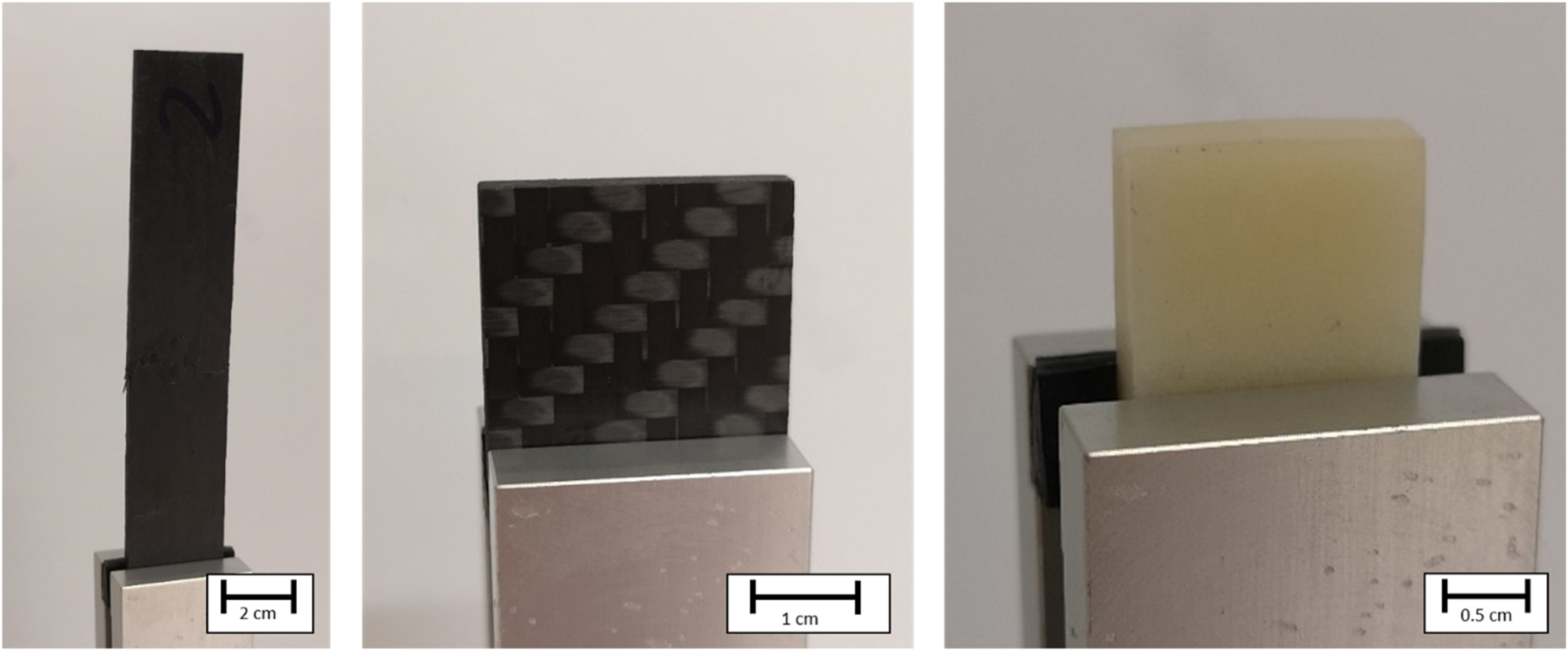
Left: recycled carbon fiber reinforced polymer specimen; middle: 8 layer carbon fiber reinforced polymer weave specimen; right: Injection molded short glass fiber reinforced polymer specimen.

2.2 Scan acquisition

The individual scans were acquired using a Lab CT (Zeiss Versa 520, see Figure 2) combining absorption and phase contrast with a voxel size of 1 µm which, together with ×4 optical magnification on a CCD detector with 2,024 × 2,024 pixels and binning equal to 1, resulting in a FOV of 2 mm × 2 mm. No filter was used for any scan. The CFRP weave specimen was scanned with an accelerating voltage of 70 kV and a power of 6 W. A total of 2,001 projections were acquired for a full rotation of 360° with an exposure time of 13 s each, resulting in a scan time of 7.2 h. The accelerating voltage and power were reduced to 65 kV and 5 W for the rCF specimen. The number of projections was 2,401 and the exposure time was 20 s, resulting in a scan time of 13.3 h. Since the injection molded specimen was thicker than the previous ones, the acceleration voltage was increased to 80 kV and the power to 7 W. 2,001 projections were recorded with an exposure time of 16 s, which was equivalent to a scan time of 8.9 h. The exposure time was chosen so that the average intensity reading of the first projection was ∼5,000. The reconstructed volumes were exported in image stacks of 1,985 images each, which corresponds to a vertical resolution of ∼1.02 µm/slice.

Figure 2:

CT scan setup: how a single scan was acquired and how the scans were overlapped.

The scans were positioned in a way that they cover the specimen from edge to edge. Depending on the thickness of the specimen, two (CFRP specimens) to four (sGFRP specimen) scans across the thickness were performed. To further increase the FOV, the same amount of horizontal scans, relative to the thickness-wide scans were chosen (see Figure 3). The single scans in the resulting grid were named according to their row and column index, starting from the top left to the bottom right (compare Figures 3, 5, 8 and 10). To minimize the overhead of redundant scanning, a small overlap of 0.1 mm was chosen.

Figure 3:

Scan acquisition (top: 2 × 2 scan setup (left: rCF specimen, right: CFRP weave specimen); bottom: 4 × 3 scan, sGFRP specimen); red: individual scans.

Since the Zeiss Xradia Versa 520 is a lab CT with a cone beam source, the perspective distortions were compensated during reconstruction, using the FDK algorithm [34], which is provided by the Zeiss Scout and Scan software (Version 16) associated with the CT [35]. In addition, this software was used to optimize the image quality, as it offers motion and beam hardening as well as ring artifact correction. This is crucial for the material elucidation in FRP, due to the low contrast of the material constituents, which requires high quality images.

2.3 Image stitching

A python script was developed for stitching the images, following two main goals. First main goal is the registration of two images and the calculation of the necessary transformation for best possible overlapping of the images. With the knowledge of the necessary transformation of the individual images, the second main goal, the stitching of the images then can be achieved. It was also necessary to ensure that the resulting images all have the same size so that the resulting image stack can be opened in programs such as Fiji [25]. For documentation purposes a metadata log-file is created. Finally, all resulting images and log files then were copied in dedicated export folders. The script is divided into five steps: Initialization of the input parameters, calculation of the transformation matrices, stitching of the images, collection of the result images and log files and padding of the result images. The images were pre-processed by histogram normalization before stitching.

The process for calculating the transformation matrices (TM) is divided into the registration of image features in the overlapping areas and the calculation of the transformation matrix from these support points. The image features are recognized using the Scale Invariant Feature Transform (SIFT) function from the python module OpenCV [36] (Version 4.8.1.78) and corresponding pairs are filtered from this set using the Fast Library for Approximate Nearest Neighbors (FLANN) module. These filtered pairs are then used as input for the estimateAffinePartial2Drigid [36] function, which calculates the affine transfer matrix TM, which takes into account rotation, scaling, and translation. Due to the high precision of the axes in the X-ray MicroCT, it can be assumed that there is no scaling of the voxels between the scans.

(1) TM = cos θ * s x − sin ⁡ θ v x sin ⁡ θ cos θ * s y v y .

θ corresponds to the angle of rotation and v to the translation in x (image row) and y (image column) direction. The translation needed is considered in the matrix elements v _x and v _y , while the scaling elements s _x and s _y are set equal to 1. The scans presented in this paper were scanned in a matrix pattern. The scan at the matrix position row and column = 0 was therefore used as a reference scan for the following operations and was not transformed. The registration and stitching was performed in pairs along the rows and columns (see Figure 4). The reference image was labeled as destination and the image to be stitched as source image.

Figure 4:

Workflow when stitching a 2 × 2 scan. First, the corresponding image feature groups are determined (green) and the TM is calculated. In the second step, the source image is transformed and stitched to the destination image (orange).

To generate the resulting image, the source, and the destination image were loaded as numpy arrays and added together. With the help of the translation entries from the TM, the overlap area and thus also the center plane(s) between the source and destination images could be determined. The destination image was cropped along center plane(s) and copied into the source image according to the calculated translations (see Figure 4). Preliminary tests showed that it was sufficiently accurate to calculate the TM only for every tenth slice and use it for the 9 following slices. This also saved computing time. During registration and stitching, metadata such as the TM, the file path of the stitched image, the file paths of the reference images, a comment on the quality of the TM and the date and time were saved in the metadata log-file. This allows the progress of the script to be tracked and individual stitches to be repeated manually, if necessary. In addition, the translation entries in the TMs could be plotted for each slice to check how the individual scans shifted in relation to each other over the slice number. For this comparison, these values were normalized to their respective starting values. In order to estimate the percentage of image area scanned multiple times, the overhead for all resulting data sets was calculated from the resulting image size A result _ image , and the total amount of scanned pixels per stitched image A individual _ image multiplied by the number of images stitched amount individual _ image

(2) Overhead = 1 − A result_image amount individual_image * A individual_image * 100 % .

3 Experimental results

The cone beam of the lab-CT X-ray source in combination with the FDK reconstruction algorithm resulted in intensity differences at the upper and lower ends of the reconstructed volume compared to its central area. Therefore, 150 slices at the upper and another 150 at the lower end were discarded, leaving 1,700 slices. This resulted in a field of view with a vertical coverage of 1,733 µm. In the following, the scans are addressed according to their position (first number = row, second number = column) in the image matrix. All datasets can be found in separate archives at ZENODO.

3.1 Recycled carbon fiber specimen (2 × 2)

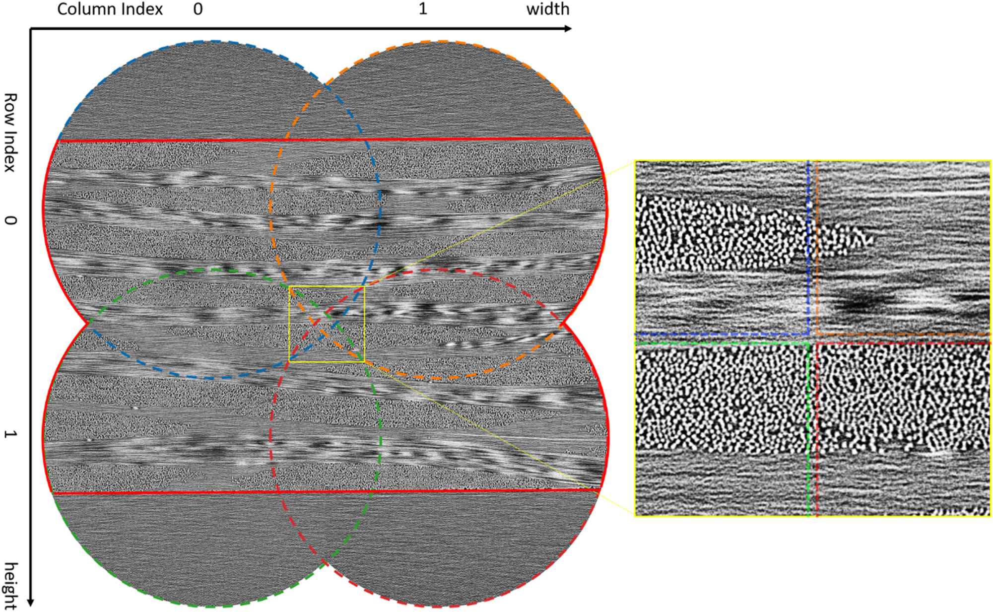
Exemplarily, the 1,000th slice of the resulting data set of the rCF specimen is shown in Figure 5. The calculated overhead is ∼23 % and the calculation time of the TMs was ∼161 min. The resulting image, with a pixel size of 1 µm² measures 3,280 × 3,276 µm², whereby the scanned specimen volume corresponds to 2,807 × 1,848 × 1,733 µm³ with a voxel size of (1 × 1 × 1.02) µm³. The complete dataset can be found at [38].

Figure 5:

Stitched slice of the 2 × 2 rCF specimen. The individual scans are framed with a dashed circle whose color corresponds to those in Figure 6. The area containing the materials information is framed in red. A coordinate system is positioned around the image in which the row and column indices as well as the direction of the height and width translations are indicated. A detailed view of the overlapping area of the 4 scans is shown on the right.

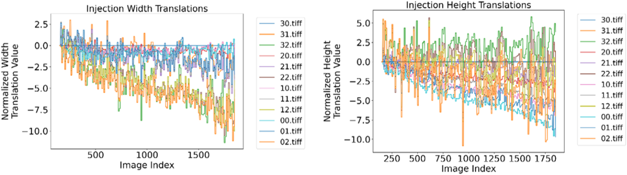
When looking at the width translations (see Figure 6), it is noticeable that scan 1–0, which was scanned in the same column as reference scan 0–0, shows no shift along the width direction. In comparison, scan 0–1, which was scanned in the same column as 0–0, shows an overall shift of ∼ −4 pixels. The plot of the height translations shows the opposite picture. Scan 0–1 shows only a very small shift, while scan 1–0 shows a total shift of ∼ −4 pixels. The shift of scan 1–1 follows the translations of its reference scans 0–1 and 1–0. To position the sample, the translation stage in width direction must change its direction of movement between scan 0–1 and 1–0, which most likely resulted in a small tilt due to reversal hysteresis of the mechanical drive.

Figure 6:

The left-hand plot shows the translations of the individual scans in the width direction as a function of the slice index. The right-hand plot shows the translations of the individual scans in the height direction as a function of the slice index.

In Figure 7 the segmentation process of the rCF specimen using the TWS [37] is illustrated. The entire stack of 1,700 images were segmented using this process resulting a calculated FVC of ∼42 %.

Figure 7:

Workflow for the TWS [37] applied to the rCF specimen images. (a) Detailed view of one cross sectional image, (b) manually labelled regions (red: fiber, green: matrix), (c) segmented image based on the manual labels from (b), the contrast difference indicates the regions, which were manually labelled and which were segmented based on these labels, (d) probability map of the fiber label. The probability map is again segmented using its histogram.

3.2 Carbon fiber weave specimen (2 × 2)

Similarly to the results of the rCF specimen, the 1,000th slice of the resulting data set of the CFRP weave specimen is shown in Figure 8. The calculated overhead was also ∼23 % and the calculation time of the TMs was ∼160 min. The resulting image sizes are equivalent to 3,267 × 3,266 µm², whereby the scanned specimen volume corresponds to 2,775 × 2,064 × 1,733 µm³ with a voxel size of (1 × 1 × 1.02) µm³. The complete dataset can be found at [39].

Figure 8:

Stitched slice of the 2 × 2 CFRP weave specimen. The individual scans are framed with a dashed circle whose color corresponds to those in Figure 9. The area containing the materials information is framed in red. A coordinate system is positioned around the image in which the row and column indices as well as the direction of the height and width translations are indicated. A detailed view of the overlapping area of the 4 scans is shown on the right.

The translation behavior of the individual scans of the CFRP weave specimen (see Figure 9) is similar to that of the rCF specimen. Similar to the scan of the rCF specimen we can observe a small tilt of the axes when changing direction with the CFRP weave specimen (see Figure 9). As there, you can see here that scan 1–0 shows no shift along the width direction, but a translation of ∼ −4 pixels in height direction. Scan 0–1 shows an overall shift of ∼ −4 pixels in width direction, but no translation in height direction. The shift of scan 1–1 follows the translations of its reference scans 0–1 and 1–0, as before.

Figure 9:

The left-hand plot shows the translations of the individual scans in the width direction as a function of the slice index. The right-hand plot shows the translations of the individual scans in the height direction as a function of the slice index.

3.3 Short glass fiber injection molded specimen (4 × 3)

Lastly, the 1,000th slice of the resulting data set of the sGFRP specimen is shown in Figure 10. The calculated overhead was due to the different scan setup at ∼32 % higher, than the previous specimens. The calculation time of the TM was also increased to ∼472 min. The resulting image sizes are equivalent to 4,622 × 4,956 µm², whereby the scanned specimen volume corresponds to 4,627 × 3,918 × 1,733 µm³ with a voxel size of (1 × 1 × 1.02) µm³. The complete dataset can be found at [40].

Figure 10:

Stitched slice of the 4 × 3 injection molded sGFRP specimen. The individual scans are framed with a dashed circle whose color corresponds to those in Figure 11. The area containing the materials information is framed in red. A coordinate system is positioned around the image in which the row and column indices as well as the direction of the height and width translations are indicated. A detailed view of the overlapping area of 4 scans (indices: 1–1, 1–2, 0–1, 0–2) is shown on the right.

The variation in translations is greater for the sGFRP specimen than for the other two specimens. Nevertheless, a similar behavior can also be seen (see Figure 11). When looking at the width translations, it is noticeable that the scans in the same column show very similar translations. For column 1, the maximum translation is ∼ −4 pixels, while that of column 2 is ∼ −8 pixels. The height translations, on the other hand, cannot be separated so clearly according to their rows. The dispersion is also significantly greater than with the width translation. In slice 940 of scan 0–2, there is also a large change in the height translation from ∼ −2 to ∼ −10 pixels. For this slice, however, the other scans show a clear shift. As scan 0–2 is the last to be stitched to the resulting image, its shift is the largest.

Figure 11:

The left-hand plot shows the translations of the individual scans in the width direction as a function of the slice index. The right-hand plot shows the translations of the individual scans in the height direction as a function of the slice index.

In Figure 12 the segmentation process of the sGFRP specimen is shown. Applying this process to the entire stack of 1,700 images, the FVC was calculated to be ∼16 % ± 2.6 %.

Figure 12:

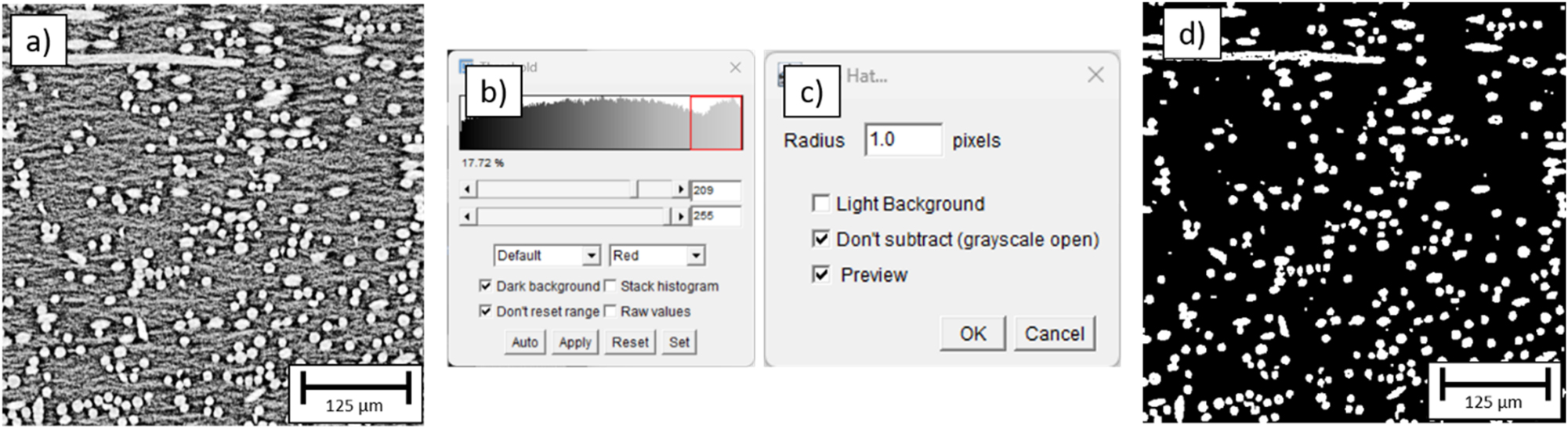
Fiber segmentation process of the sGFRP specimen. (a) Detailed view of a cross sectional image, (b) settings for the histgram segmentation (treshold = 209), (c) settings for the top hat filter, (d) segmentation result.

4 Discussion

The stitched image of the rCF sample clearly shows that the entire cross-section of the sample is imaged resulting in a volume of 2,747 × 1,879 × 1,733 µm³ with a voxel size of (1 × 1 × 1.02) µm³. This enables not only to segment individual fibers, but also to analyze the path of the fiber bundles. A similar result can be seen in the stitched image of the CFRP weave specimen, where the resulting volume has a size of 2,729 × 2,059 × 1,733 µm³ with a voxel size of (1 × 1 × 1.02) µm³. Segmenting this volume using the TWS [37] and histogram tresholding, a FVC of ∼42 % could be calculated. A comparison with the experimentally determined values (43–47 %) from [33] shows that the result of the segmentation corresponds well with the values of similarly produced rCF test specimens. It is noticeable that the individual layers slid into each other during production, deviating from the ideal model. In between the rovings, matrix-rich regions formed (see Figure 8). Due to the low contrast and complex weaved roving structure, the exact segmentation into 0° and 90° rovings, as well as detecting matrix-rich zones, is still part of the ongoing research [41]. The stitching of the 12 ROI scans of the sGFRP specimen resulted in a volume of 4,348 × 3,923 × 1,733 µm³ with a voxel size of (1 × 1 × 1.02) µm³. Due to the high contrast in the stitched images, a histogram segmentation followed by a filtering step was sufficient to calculate a FVC of ∼16 % ± 2.6 %. This relatively high error results from two sources in the histogram-based segmentation. Firstly, small changes in the lower boundary of the grey value can result in a great difference of the FVC. In this case, Otsu’s method [42] did not achieve satisfying results, which is why the lower boundary was set manually. The second source of errors is attributed to the phase contrast imaging. At the borders of the material phases, X-ray phase fringes form, which is by design, but it also leads to fiber volume estimation errors [43], [44].

The sectional view of the sGFRP sample shows how the molding conditions during the injection process influence the position and orientation of the glass fibers in the finished component, resulting in a characteristically layered structure.

When viewing the interface areas in Figures 5, 8 and 10, only minimal stitching artifacts can be seen, although the imagses were only pasted on top of each other and no blending or other processing of the interface area was performed. Low-artifact stitching is particularly important for fiber structures, as these can otherwise impair the segmentation of the individual fibers. This could be achieved through the high image quality and the preprocessing of the images. Preliminary tests showed that the SIFT function used was only able to recognize corresponding image areas in the source and destination image after the histogram normalization of the images. In addition, the histogram normalization led to the gray value distributions of the individual scans being adjusted to each other. This enables easier segmentation, as the gray value distributions of the material features, such as fibers, matrix or pores, were qualitatively very similar in the individual scans but differed quantitatively from each other due to offsets.

The displacement error of the individual scans is very low compared to the size of the resulting image at <0.25 %, which indicates a high precision of the mechanical axes in the CT used. The observed displacements shown in Figures 6, 9 and 11 cannot be assigned to one specific cause as they result from a superposition of several phenomena.

Firstly, the machine axes have an inherent approach-inaccuracy and a slight tilting which changes direction as soon as the axes change their direction of travel. This happens when moving to the first width position (i.e. moving back) after changing to the next height position. Secondly, the errors are cumulative, the new reconstructions are still referenced to the first one during stitching, so the error increases as the number of travels increases. Thirdly, the source, the sample stage and the detector have small positioning and alignment errors in relation to each other. A translation in the row index therefore results in a change in the distance of the already recorded areas (the overlap) to the source & detector, which leads to a shift of the projected image in the event of alignment errors. And fourthly, the Zeiss reconstruction algorithm apparently uses dithering between the projections and has drift compensation for reconstruction, which can also result in a shift of the reconstructed volumes.

High image quality also turned out to be very important for precise registration. As the images are stitched one after the other and errors therefore propagate if registration is inaccurate. The evaluation of the resulting image stack of cross-sections easily reveals such precision of the alignment of the individual scans to each other. Based on this observation a limit of ±0.1 % was implemented as threshold for the deviation of the TM values for rotation in Eq. (1). Exceeding this threshold is recorded in the metadata log file with a comment.

5 Conclusion and outlook

Using the Zeiss Versa 520 in phase contrast mode, specimens of three distinct types of composite material could be scanned with a voxel resolution of 1 µm/voxel and high sharpness of separation despite the low absorption and the small difference in absorption between fiber, matrix, and pores. After histogram normalization, it was therefore possible to calculate the rotations and translations for the registration of the overlapping scans in a script developed for this purpose. The scans could then be stitched with minimal artifacts to achieve very large fields of view with voxel counts of approx. 3,280 × 3,276 × 1,700 ≈ 9.0 × 10⁹ for the rCF specimen, 2,775 × 2,064 × 1,700 ≈ 9.9 × 10⁹ for the CFRP weave specimen and 4,627 × 3,918 × 1,700 ≈ 3.1 × 10¹⁰ for the sGFRP specimen. Meanwhile, metadata files were automatically generated, and the resulting images were padded to the identical size. The goal of increasing the FOV of low-absorbing FRP samples with the help of a lab CT could thus be achieved. Since the duration of the stitching of two scans took less time than the acquisition of another scan, the computing time of the stitching was of secondary priority. However, in order to optimize the method presented here in the future, it may make sense to scan in an octahedral pattern [13] instead of a matrix pattern. In addition, the small stitching artifacts can be reduced if the images are split using a graph cut [22].

References

[1] P. J. Withers, et al.., “X-ray computed tomography,” Nat. Rev. Methods Primers, vol. 1, no. 1, p. 18, 2021, https://doi.org/10.1038/s43586-021-00015-4.Suche in Google Scholar
[2] O. Wirjadi, et al.., “Characterization of multilayer structures in fiber reinforced polymer employing synchrotron and laboratory X-ray CT,” Int. J. Mater. Res., vol. 105, no. 7, pp. 645–654, 2014, https://doi.org/10.3139/146.111082.Suche in Google Scholar
[3] F. Léonard, J. Stein, C. Soutis, and P. J. Withers, “The quantification of impact damage distribution in composite laminates by analysis of X-ray computed tomograms,” Compos. Sci. Technol., vol. 152, pp. 139–148, 2017, https://doi.org/10.1016/j.compscitech.2017.08.034.Suche in Google Scholar
[4] L. Zhou, A. Mehta, B. McWilliams, K. Cho, and Y. Sohn, “Microstructure, precipitates and mechanical properties of powder bed fused inconel 718 before and after heat treatment,” J. Mater. Sci. Technol., vol. 35, no. 6, pp. 1153–1164, 2019, https://doi.org/10.1016/j.jmst.2018.12.006.Suche in Google Scholar
[5] J. Jungbluth, et al.., “Interface failure analysis of embedded NiTi SMA wires using in situ high-resolution X-ray synchrotron tomography,” Mater. Char., vol. 205, p. 113345, 2023. https://doi.org/10.1016/j.matchar.2023.113345.Suche in Google Scholar
[6] E. Maire, J. Y. Buffière, L. Salvo, J. J. Blandin, W. Ludwig, and J. M. Létang, “On the application of X-ray microtomography in the field of materials science,” Adv. Eng. Mater., vol. 3, no. 8, pp. 539–546, 2001, https://doi.org/10.1002/1527-2648(200108)3:8<539::AID-ADEM539>3.0.CO;2-6.10.1002/1527-2648(200108)3:8<539::AID-ADEM539>3.0.CO;2-6Suche in Google Scholar
[7] F. Pfeiffer, T. Weitkamp, O. Bunk, and C. David, “Phase retrieval and differential phase-contrast imaging with low-brilliance X-ray sources,” Nat. Phys, vol. 2, no. 4, pp. 258–261, 2006, https://doi.org/10.1038/nphys265.Suche in Google Scholar
[8] A. V. Bronnikov, “Phase-contrast CT: fundamental theorem and fast image reconstruction algorithms,” in Optics + Photonics, U. Bonse, Ed., San Diego, California, USA, SPIE, 2006, p. 63180Q.10.1117/12.679389Suche in Google Scholar
[9] O. Brunke, et al.., “Comparison between X-ray tube-based and synchrotron radiation-based μCT,” in Optical Engineering + Applications, S. R. Stock, Ed., San Diego, California, USA, SPIE, 2008, p. 70780U.10.1117/12.794789Suche in Google Scholar
[10] J. Kastner, B. Harrer, G. Requena, and O. Brunke, “A comparative study of high resolution cone beam X-ray tomography and synchrotron tomography applied to Fe- and Al-alloys,” NDT E Int., vol. 43, no. 7, pp. 599–605, 2010, https://doi.org/10.1016/j.ndteint.2010.06.004.Suche in Google Scholar
[11] A. Kyrieleis, M. Ibison, V. Titarenko, and P. J. Withers, “Image stitching strategies for tomographic imaging of large objects at high resolution at synchrotron sources,” Nucl. Instrum. Methods Phys. Res. Sect. A Accel. Spectrom. Detect. Assoc. Equip., vol. 607, no. 3, pp. 677–684, 2009, https://doi.org/10.1016/j.nima.2009.06.030.Suche in Google Scholar
[12] S. Englisch, J. Wirth, D. Drobek, B. Apeleo Zubiri, and E. Spiecker, “Expanding accessible 3D sample size in lab-based X-ray nanotomography without compromising resolution,” Precis. Eng., vol. 82, pp. 169–183, 2023, https://doi.org/10.1016/j.precisioneng.2023.02.011.Suche in Google Scholar
[13] M. Fransson, B. Cordonnier, R. Zimmermanns, P. R. Shearing, A. Rack, and L. Broche, “A comparison of stitching techniques to reconstruct large volume X-ray tomography of batteries,” Tomography Mater. Structures, vol. 5, p. 100029, 2024, https://doi.org/10.1016/j.tmater.2024.100029.Suche in Google Scholar
[14] M. Kimura, T. Watanabe, Y. Takeichi, and Y. Niwa, “Nanoscopic origin of cracks in carbon fibre-reinforced plastic composites,” Sci. Rep., vol. 9, no. 1, p. 19300, 2019, https://doi.org/10.1038/s41598-019-55904-2.Suche in Google Scholar PubMed PubMed Central
[15] M. Kimura, et al.., “Nanoscale in situ observation of damage formation in carbon fiber/epoxy composites under mixed-mode loading using synchrotron radiation X-ray computed tomography,” Compos. Sci. Technol., vol. 230, p. 109332, 2022, https://doi.org/10.1016/j.compscitech.2022.109332.Suche in Google Scholar
[16] N. Pournoori, et al.., “In situ damage characterization of CFRP under compression using high-speed optical, infrared and synchrotron X-ray phase-contrast imaging,” Compos. Appl. Sci. Manuf., vol. 175, p. 107766, 2023, https://doi.org/10.1016/j.compositesa.2023.107766.Suche in Google Scholar
[17] O. Brunke, “High-resolution CT-based defect analysis and dimensional measurement,” Insight, vol. 52, no. 2, pp. 91–93, 2010. https://doi.org/10.1784/insi.2010.52.2.91.Suche in Google Scholar
[18] G. R. Davis and J. C. Elliott, “Artefacts in X-ray microtomography of materials,” Mater. Sci. Technol., vol. 22, no. 9, pp. 1011–1018, 2006, https://doi.org/10.1179/174328406X114117.Suche in Google Scholar
[19] V. Van Nieuwenhove, J. De Beenhouwer, F. De Carlo, L. Mancini, F. Marone, and J. Sijbers, “Dynamic intensity normalization using eigen flat fields in X-ray imaging,” Opt. Express, vol. 23, no. 21, p. 27975, 2015, https://doi.org/10.1364/OE.23.027975.Suche in Google Scholar PubMed
[20] D. John, et al.., “Centimeter-sized objects at micrometer resolution: extending field-of-view in wavefront marker X-ray phase-contrast tomography,” 2024. arXiv: arXiv:2408.00482 [Online]. Available at: http://arxiv.org/abs/2408.00482 Accessed: Aug. 29, 2024.Suche in Google Scholar
[21] D. Rueckert, L. I. Sonoda, C. Hayes, D. L. G. Hill, M. O. Leach, and D. J. Hawkes, “Nonrigid registration using free-form deformations: application to breast MR images,” IEEE Trans. Med. Imaging, vol. 18, no. 8, pp. 712–721, 1999, https://doi.org/10.1109/42.796284.Suche in Google Scholar PubMed
[22] I. V. Oikonomidis, et al.., “Imaging samples larger than the field of view: the SLS experience,” J. Phys. Conf. Ser., vol. 849, no. 1, p. 012004, 2017. https://doi.org/10.1088/1742-6596/849/1/012004.Suche in Google Scholar
[23] C. D. Kuglin and D. C. Hines, “The phase correlation image alignment method,” in Proceedings of the IEEE, Bd. International Conference on Cybernetics and Society, pp. 163–165.Suche in Google Scholar
[24] D. G. Lowe, “Distinctive image features from scale-invariant keypoints,” Int. J. Comput. Vis., vol. 60, no. 2, pp. 91–110, 2004, https://doi.org/10.1023/B:VISI.0000029664.99615.94.10.1023/B:VISI.0000029664.99615.94Suche in Google Scholar
[25] J. Schindelin, et al.., “Fiji: an open-source platform for biological-image analysis,” Nat. Methods, vol. 9, no. 7, pp. 676–682, 2012, https://doi.org/10.1038/nmeth.2019.Suche in Google Scholar PubMed PubMed Central
[26] S. Preibisch, S. Saalfeld, and P. Tomancak, “Globally optimal stitching of tiled 3D microscopic image acquisitions,” Bioinformatics, vol. 25, no. 11, pp. 1463–1465, 2009, https://doi.org/10.1093/bioinformatics/btp184.Suche in Google Scholar PubMed PubMed Central
[27] A. Miettinen, I. V. Oikonomidis, A. Bonnin, and M. Stampanoni, “NRStitcher: non-rigid stitching of terapixel-scale volumetric images,” Bioinformatics, vol. 35, no. 24, pp. 5290–5297, 2019, https://doi.org/10.1093/bioinformatics/btz423.Suche in Google Scholar PubMed
[28] A. Baumann and J. Hausmann, “Effect of high-energy radiation on the relaxation of residual stresses in polycarbonate and epoxy resin by stress optics,” Radiat. Phys. Chem., vol. 226, p. 112236, 2025, https://doi.org/10.1016/j.radphyschem.2024.112236.Suche in Google Scholar
[29] R. Hartley and A. Zisserman, Multiple View Geometry in Computer Vision, Cambridge, United Kingdom, Cambridge University Press, 2003.10.1017/CBO9780511811685Suche in Google Scholar
[30] C. Ji, “Accurate 3D data stitching in circular cone-beam micro-CT,” J. X-Ray Sci. Technol., vol. 18, no. 2, pp. 99–110, 2010, https://doi.org/10.3233/XST-2010-0246.Suche in Google Scholar PubMed
[31] J. Llorca, et al.., “Multiscale modeling of composite materials: a roadmap towards virtual testing,” Adv. Mater., vol. 23, no. 44, pp. 5130–5147, 2011, https://doi.org/10.1002/adma.201101683.Suche in Google Scholar PubMed
[32] E. Syerko, et al.., “Benchmark exercise on image-based permeability determination of engineering textiles: microscale predictions,” Compos. Appl. Sci. Manuf., vol. 167, p. 107397, 2023, https://doi.org/10.1016/j.compositesa.2022.107397.Suche in Google Scholar
[33] M. Detzel, P. Mitschang, and U. Breuer, “New approach for processing recycled carbon staple fiber yarns into unidirectionally reinforced recycled carbon staple fiber tape,” Polymers, vol. 15, no. 23, p. 4575, 2023, https://doi.org/10.3390/polym15234575.Suche in Google Scholar PubMed PubMed Central
[34] L. A. Feldkamp, L. C. Davis, and J. W. Kress, “Practical cone-beam algorithm,” J. Opt. Soc. Am. A., vol. 1, no. 6, p. 612, 1984, https://doi.org/10.1364/JOSAA.1.000612.Suche in Google Scholar
[35] Carl Zeiss Microscopy Deutschland GmbH, Scout and Scan Version 16, Oberkochen, Germany, Carl Zeiss Microscopy Deutschland GmbH, 2019.Suche in Google Scholar
[36] G. Bradski, “The OpenCV library,” Dr. Dobb’s J. Softw. Tools, vol. 25, no. 11, pp. 120–123, 2000.Suche in Google Scholar
[37] I. Arganda-Carreras, et al.., “Trainable weka segmentation: a machine learning tool for microscopy pixel classification,” Bioinformatics, vol. 33, no. 15, pp. 2424–2426, 2017, https://doi.org/10.1093/bioinformatics/btx180.Suche in Google Scholar PubMed
[38] B. Boos, C. Queck, and M. Gurka, “Recycled carbon fiber reinforced composites: stitched lab X-ray CT scan images to increase field of view,” 2025, https://doi.org/10.5281/zenodo.14945398.Suche in Google Scholar
[39] B. Boos, C. Queck, and M. Gurka, “Carbon fiber reinforced twill weave composite: stitched lab X-ray CT scan images to increase field of view,” 2025, https://doi.org/10.5281/zenodo.14946081.Suche in Google Scholar
[40] B. Boos, C. Queck, and M. Gurka, “Injection molded short fiber reinforced composites: stitched lab X-ray CT scan images to increase field of view,” 2025, https://doi.org/10.5281/zenodo.14945626.Suche in Google Scholar
[41] B. Boos, K. Chen, A. Gebhard, and M. Gurka, “Segmentation of a CFRP weave structure for material characterization and simulation,” eJNDT, vol. 30, no. 2, 2025, https://doi.org/10.58286/30714.Suche in Google Scholar
[42] N. Otsu, “A threshold selection method from gray-level histograms,” IEEE Trans. Syst., Man, Cybern., vol. 9, no. 1, pp. 62–66, 1979, https://doi.org/10.1109/TSMC.1979.4310076.Suche in Google Scholar
[43] T. W. Way, et al.., “Effect of CT scanning parameters on volumetric measurements of pulmonary nodules by 3D active contour segmentation: a phantom study,” Phys. Med. Biol., vol. 53, no. 5, pp. 1295–1312, 2008, https://doi.org/10.1088/0031-9155/53/5/009.Suche in Google Scholar PubMed PubMed Central
[44] F. Heckel, et al.., “Segmentation-based partial volume correction for volume estimation of solid lesions in CT,” IEEE Trans. Med. Imaging, vol. 33, no. 2, pp. 462–480, 2014, https://doi.org/10.1109/TMI.2013.2287374.Suche in Google Scholar PubMed
© 2025 the author(s), published by De Gruyter on behalf of Thoss Media
This work is licensed under the Creative Commons Attribution 4.0 International License.