Separating disease and health for indirect reference intervals
-
Kenneth A. Sikaris


Abstract
The indirect approach to defining reference intervals operates ‘a posteriori’, on stored laboratory data. It relies on being able to separate healthy and diseased populations using one or both of clinical techniques or statistical techniques. These techniques are also fundamental in a priori, direct reference interval approaches. The clinical techniques rely on using clinical data that is stored either in the electronic health record or within the laboratory database, to exclude patients with possible disease. It depends on the investigators understanding of the data and the pathological impacts on tests. The statistical technique relies on identifying a dominant, apparently healthy, typically Gaussian distribution, which is unaffected by the overlapping populations with higher (or lower) results. It depends on having large databases to give confidence in the extrapolation of the narrow portion of overall distribution representing unaffected individuals. The statistical issues involved can be complex, and can result in unintended bias, particularly when the impacts of disease and the physiological variations in the data are under appreciated.
Introduction
Diagnostic testing essentially aims to support the clinician in answering specific clinical questions. While many of these diagnostic queries are usually aimed at answering the question “Is disease present?”, the simplest interpretative tool provided on reports, the reference interval, has only an indirect relationship to identifying disease. The reference interval describes the confidence limits based on the typical values found in apparent health, or the absence of disease, and therefore only directly answers the question “Is health likely to exist?” Therefore, reference intervals identify the apparently healthy population and must be distinguished from ‘clinical decision limits’ that more appropriately identify the values in a specified diseased population. These are fundamental issues which are often poorly appreciated so the International Federation of Clinical Chemistry and Laboratory Medicine (IFCC) Committee on Reference Intervals and Decision Limits (C-RIDL) have recently published a position statement around this distinction [1].
Laboratorians may be familiar with receiver operator characteristic (ROC) curves that decrease the specificity for health against the sensitivity for disease (or vice versa), in order to define a cut-off that has intermediate specificity and sensitivity. It is important to acknowledge that ROC cut-offs are not reference intervals, which are, by definition, solely concerned with specificity for an apparently healthy reference population.
The object of this discussion is to address the methodological issues in deriving ‘indirect’ reference intervals. Direct reference interval studies aim to identify a population of healthy individuals ‘a priori’, and then describe the confidence limits of their distribution of results. Indirect reference intervals aim to identify the apparently healthy distribution of results ‘a posteriori’ from a database that includes both healthy and diseased individuals [2]. Whilst indirect approaches are relatively convenient and cheap to do, it is obvious that dealing with a mixed population is far more difficult than dealing with a homogenous healthy population, and therefore any tools that are used to separate healthy and diseased distributions must be understood, and applied with high degree of rigour, if a reliable indirect reference interval is the aim.
Indirect reference interval databases
While all indirect reference intervals are derived from a mixture of healthy and diseased individuals, the prevalence of disease in the database can vary considerably. Indirect reference intervals can be derived from cross sectional population studies, such as NHANES [3], [4], [5], which contain the background community prevalence of all diseases. The community prevalence of disease might be assumed to be low, however common diseases such as diabetes are often present in over 10% of the population in many developing and developed countries, and many studies find it necessary to exclude large proportions of the general population on the basis of supplied medical history and outlier observations. Clinical laboratory result databases from tertiary medical facilities, such as teaching hospitals, are at the other extreme of disease prevalence, including the high prevalence of disease amongst inpatients, as most patients have an illness as the reason for their admission. One of largest and most useful clinical databases for indirect reference intervals is that of primary care clinical laboratories. Ambulant ‘patients’ have will either have milder disease than their inpatient counterparts, or they don’t have disease and are having check-ups to monitor their risk of disease. These very large databases have disease prevalence that is closer to the background disease prevalence of general community.
There is an acknowledged international standard for defining reference intervals which is published by the Clinical Laboratory Standards Institute (CLSI) and endorsed by the IFCC [6]. The standard mentions that the best data for a posteriori studies would be from apparently healthy individuals who would by definition be asymptomatic and having health screening e.g. occupational screening or genetic screening or routine clinical screening before blood donations or minor surgical procedures.
Clearly, the higher the prevalence of diseased individuals in the database, the greater the effort required in separating healthy and diseased individuals. One of the main reasons that this may not be as problematic as it appears is that any particular test is not affected by all diseases. For example, diabetes does not usually increase prostate specific antigen (PSA) [7], nor are glucose levels related to prostate cancer mortality [8]. Thus tests which are unaffected by the disease (or its treatment) in a patient may be considered to represent a healthy state.
Strategies
The strategies for distinguishing healthy individuals from diseased individuals using the indirect approach are fundamentally exactly the same as for direct reference interval determinations. These strategies can either have a clinical or statistical basis.
The CLSI standard [6] states that the designation of good health for a candidate reference individual can include either clinical criteria such as history, physical examinations or laboratory criteria such as the results of clinical laboratory tests. As an example, to formally establish direct reference intervals for testosterone, we took clinical histories and examined 124 young men, including orchidometry, as well as performing semen analysis on all these men to a priori exclude testicular insufficiency [9]. I will discuss (below) the equivalent of taking a clinical history and examination or performing relevant clinical laboratory tests using the a posteriori indirect approach.
As well as seeking the clinical evidence from history, examination and testing, there is also a statistical strategy applied direct reference interval definition which includes applying parametric, or non-parametric, assumptions to the reference distributions and identifying statistical outliers. These are also vitally important considerations when defining indirect reference intervals.
Strategies can be both clinical and statistical and we will discuss how limiting the number of results from each individual reduces statistical bias as well as reducing clinical bias because diseased individuals often have more results.
Strategic pre-requisites for the indirect approach
Farrell and Nguyen [10] have pointed out that it is essential to check for pre-analytical and analytical artifacts prior to using any laboratory data. Pre-analytical factors, such as sampling time, sampling tubes and sample transport and storage prior to analysis must be understood and be consistent over time. Secondly, analytical factors such as assay manufacturer and calibration must also be consistent. This is relatively easy to check for as a review of monthly means [11] (or medians) over the course of the study should highlight any shifts in the data that need to be taken into account. Internal quality control and external quality assurance (EQA) will also give greater confidence in analytical stability as well as supporting the transference of any reference interval determined. Shifts of the result distributions are assumed to be due to analytical and pre-analytical factors, but can occasionally be due to population shifts, if the laboratory has a significant change in patient characteristics. The longitudinal trends in the data also have an extra advantage because circannual variations can often be seen as expected for vitamin D [12] and less expected analytes such as HbA1c [13] and routine chemistry [14], [15]. It is therefore desirable that the data avoid circannual effects by having a database that includes multiples of a whole year. All laboratories could consider routinely auditing their result distributions, including flag rates, to confirm that their methods are stable as well as confirming that their reference intervals are still appropriate. I am often extracting data in response to clinical ‘complaints’ that they are seeing an increase in abnormalities. Similarly, if EQA reveals a potential shift in patient’s results, a review of result distributions and flag rates will usually reveal any significant concerns.
Clinical strategies for identifying underlying disease
Clinical history (and examination)
Optimal pathology request forms include clinical notes supplied by the clinician that include the clinical reasons for testing. These notes were ultimately derived from the observations elicited in the history and examination. Absence of clinical notes from a request form does not equate with absence of purpose for testing, simply that the purpose wasn’t conveyed to the laboratory. The nature of clinical notes clearly impact the abnormality rate of a test [16], [17]. Figure 1 shows two distributions of serum luteinising hormone (LH) levels measured in 40–45 years old women. One distribution is from women with regular periods indicated by the stated day of their cycle on the request form (e.g. Day 2 or 7 or 21), whereas the other was from women who were indicated to be possibly menopausal e.g. flushing. This demonstrates how data distributions can be selective for unaffected individuals simply using supplied request form clinical notes. Thyroid tests are usually accompanied with an indication of whether the patient is taking thyroid medication, and these patients should be excluded when deriving thyroid test reference limits [18], [19], but ideally linking with a pharmacy database may give greater confidence (than the limited information on the request form) in excluding patients on thyroid medications [20].
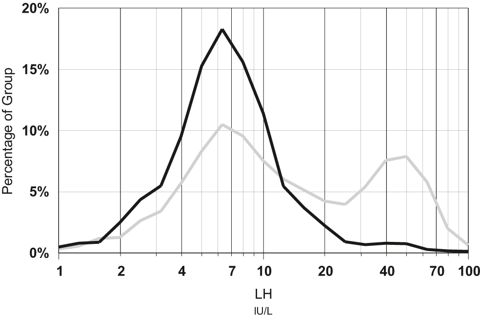
Distribution of luteinising hormone (LH) results for 9,684 women aged 40–45 years, with the day of their period indicated on the request form (black line) compared to distribution of 4,295 women with clinical notes indicating flushing or possible menopause (grey line).
LH was measured on Roche Elecsys over the period 2010–2020 in a community based laboratory.
Some examination findings would be particularly helpful when deriving reference limits especially anthropometric measures that might indicate obesity, or blood pressure results. These are sometimes unavailable in the clinic, let alone in the laboratory, but some laboratories can collect these important measurements [21]. Obesity is a common cause for skewness for numerous common biochemical analytes [22], [23], [24], [25], and this is often a neglected issue for both indirect and direct reference limit estimation [26].
Other forms of clinical exclusion of indirect data include using stored medical and hospital diagnostic information [27]. For example, if trying to derive reference intervals for renal tests, it would be useful to exclude patients from renal wards or patients who were admitted or discharged with a diagnosis of renal disease. It will be difficult to enumerate and exclude all the possible clinical causes of a particular test abnormality [28] unless all that clinical information is captured. The Laboratory Information Mining for Individualised Thresholds (LIMIT) method systematically identifies ICD9 disease codes associated with extreme results and then excludes individuals having these codes in an iterative manner [29]. It is logical that patients with hospital ICD9 codes of anaemia, blood transfusion and surgical procedures are easily identifiable as populations with a large proportion of outlier haemoglobin levels, so they can be excluded.
Clinical laboratory tests
Tests are not only performed for diagnostic purposes but also for screening and monitoring, therefore analysis of laboratory data needs to be conducted with awareness of these separate contexts in order to identify and mitigate potential biases in the data [30]. Patients having multiple tests, are more likely to be monitored for disease, therefore excluding patients with numerous results (e.g. more than three) [31], or including only a single result per patient (typically the first) [26], or even more thoroughly, limiting only to individuals having a single test in the study period [32]. Figure 2 shows the increasing likelihood that adults between the age of 18 and 65 years will have repeat measurements of serum creatinine within 12 months, when the initial creatinine lies outside their respective gender related reference interval. Patients having follow up testing due to previous abnormalities can also cause irregular distributions which is another strong reason to exclude them [33].
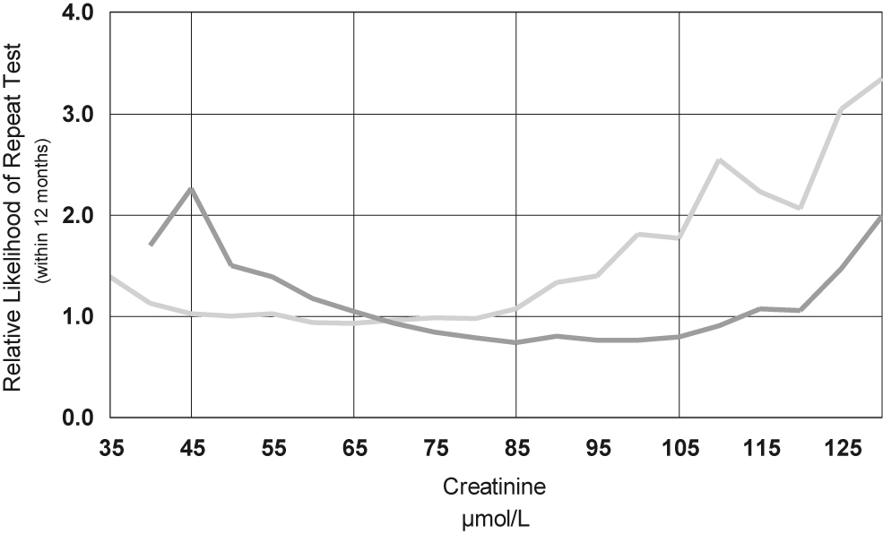
Relative likelihood of repeat testing within 12 months of serum creatinine against the initial creatinine result for 530,000 women (light coloured line) and 430,000 men (dark coloured line).
The creatinine reference interval for women (Roche enzymatic method) is 45–85 μmol/L for women and 65–105 μmol/L for men.
Co-requested tests are a particularly useful strategy for the indirect approach. It is logical to insist that patients selected for potassium reference interval determinations do not have a low estimated glomerular filtration rate (eGFR) indicative of renal failure. Selectivity can be increased by using the results of multiple tests, such as when deriving an indirect reference interval for parathyroid hormone (PTH), where not only renal function (eGFR) should be normal, but also that calcium and vitamin D levels should be normal [34]. Similarly, tests that are affected by inflammation could be selected from patients that have normal co-requested C-reactive protein (CRP) levels. Figure 3 shows that patients with elevated serum CRP skew the results for serum alpha-1-antitrypsin (A1AT) and therefore using only A1AT results from patients with a normal CRP give a more healthy distribution. This may rely on a clinical understanding of the associations of all tests with disease or a learning strategy from the statistical evidence that the analyte of interest is correlated with other measures of disease [35]. A similar learning strategy is to exclude all patients having repeated co-requested tests within a short time interval because repeated testing, regardless of the results, is more likely to be associated with disease [36].
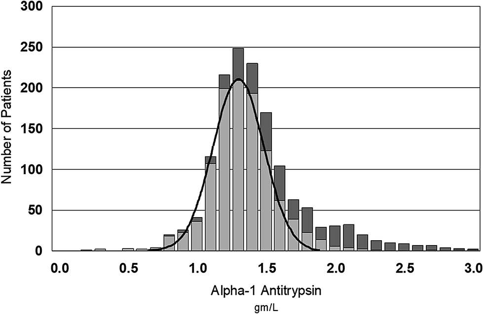
Gaussian distribution of alpha-1-antitrypsin (A1AT) levels in 1,125 patients with normal C-reactive protein (CRP) (≤5 mg/L, light bars) compared to higher levels of A1AT in 475 patients with raised CRP (dark bars).
CRP and A1AT were measured using a Roche immunoturbidimetric method.
Statistical strategies for identifying underlying disease
The dominant statistical strategy for isolating indirect reference intervals is that all reference distributions are Gaussian, or log Gaussian. I will also address my cautionary view regarding the assumption of other distributions. Non-parametric approaches are uncommon and include Piecewise Regression that operates on non-parametric percentile analysis to identify partitioning ‘break points’ which are assumed to reflect normal physiology, but therefore rely heavily on clinical disease exclusion criteria [5].
The confidence that Gaussian distributions explain reference intervals may seem like a divine belief in the beauty and symmetry of the Gaussian curve, however there is something fundamentally ‘natural’ in the Gaussian curve which reflects the diversity of nature. If we explore the distributions of chance, moving from binomial distribution (e.g. tossing a coin), to multiple determinants of chance (e.g. tossing 20 coins), the distributions gradually become Gaussian [37]. Therefore a Gaussian reference interval reflects the many factors (usually >>20) that cause variation of results between healthy individuals. This is no different to what laboratory scientists intrinsically understand regarding analysis, where measurement uncertainty follows the Gaussian distribution because there are numerous determinants that affect every step in analysis including calibration errors, sampling errors, lot to lot reaction variations and reading errors. Even when measurement uncertainty is very small, it follows a Gaussian distribution.
The Gaussian distribution of results from a reference population includes not only the Gaussian analytical variation in each result, but also the intraindividual and interindividual variations which are, according to the assumptions of biological variability, also Gaussian [38]. Intraindividual changes have a multiple determinants including hydration status, diurnal variation, circannual variations, as well as the various effects of daily diet, activity and stress. Interindividual differences are as varied as our unique physical appearances and height, weight and body mass index (BMI) were some of the historical measures demonstrated by Quetelet to follow Gaussian distributions [39].
Log Gaussian transformations
Skewed distributions represent the dominance of at least one variability factor in one direction. A common example of skewed results seems to be because many substances appear in the blood much faster than the rate at which they fall (e.g. hormones, enzymes and tumour markers) and as a result, all of these substances have a skewed distribution to the right. We know the appearance or disappearance of these analytes can be described by doubling times or half-lives, so we should not be surprised that these distributions are logarithmically skewed. Logarithmic transformation could therefore be applied when analyte skewness is explainable by such exponential considerations (i.e. doubling time or half-life). Log transformation is the most relevant transformation for biological results [40] and has therefore been defined as the ‘biological hypothesis’ [41]. Log transformation has little effect on tight distributions and is a good approximation for many broadly skewed distributions, which may be why it seems a universal transformation.
Complex Gaussian transformations
A particular variation of logarithmic transformation includes adding a small constant to the data (log[x + c]), but this empirical method of improving skewness can have major impacts on the statistical conclusions from the data [42], as well as having no pathophysiological theory for explaining why it should be applied. Transformations using log[x + c] can ‘successfully’ remove skewness [43], however they may also normalise expected gender differences e.g. creatine kinase levels. Power normal distributions, including the ‘Box–Cox’ transformation ([x λ − 1]/λ) [44], are even more effective at normalising a skewed distribution but even Box and Cox warned that “the reasonable thing will often be first to apply the transformations suggested by the prior reasoning, and after that consider what further modifications, if any, are needed”. An example of a ‘transformation suggested by prior reasoning’ may be to use a lambda value that has been determined in a relevant a priori reference interval study. When the Box–Cox λ coefficient equals one, the distribution is normal and if λ coefficient is zero, the distribution is a log normal distribution. Other values of λ assume a distribution which is neither normal Gaussian or log normal Gaussian and may provide a better overall fit but can have major impacts on the derived reference limits [45] and lead to inconsistencies when compared to direct reference intervals. Additionally, applying two stage Gaussian transformations have also been shown to potentially reduce the goodness of fit of the data compared to non-transformed [46].
Non-Gaussian distributions
Other distributions that could potentially be adapted to fit the reference distribution data include exponential, Chi-squared and Erlang distributions, which all belong to the gamma distribution family which are described by varying ‘shape’ and ‘scale’ parameters. Gamma distributions, which are often used in economics and marketing can be applied to health data [47]. An iterative gamma distribution approach can be used to improve the fit of reference distribution data, however, as the authors of a Dutch study of folate reference intervals acknowledge, their gamma fitting incorporated the population of individuals taking supplements that could have normally been considered as outliers [48].
In general, complex Gaussian and non-Gaussian transformations do not usually make large differences in reference limit determination, unless the skewness coefficient of the reference data is large (>0.6) or kurtosis coefficient is high (>2.7) [49]. Simple logarithmic transformation is usually all that is required, and Box–Cox methods usually provide better normalisation of the data but the improvements are usually small [50], and come with the risk of including diseased individuals in the reference population. For example, the typically log normal distribution of alkaline phosphatase (ALP) might be inadvertently extended to include patients with vitamin D deficiency [51].
The issue of avoiding inadvertent extension of the reference interval is of special relevance in the subject of this paper, because we are aiming to separate healthy and diseased distributions and complex transformations can normalise overlapping healthy and diseased populations, which certainly undermines the specificity of indirect reference intervals.
Latent class distribution regression is another new method which assumes that an underlying Gaussian population can be differentiated from a latent diseased population [52]. Although initially applied to analytes that either increase or decrease in the presence of disease, there is no statistical reason why this cannot be applied to analytes that may vary in both directions with disease. As might be expected, this method is most efficient when disease causes a large distribution shift and can overestimate reference limits when the shift is subtle and the overlap is large.
Eliminating outliers
Many outlier exclusion techniques assume Gaussian distributions and rely on eliminating data whose distance from the mean (usually expressed as multiples of standard deviations), is more frequent than would be predicted by the size of the study population. Examples include Chauvenet’s criterion, Peirce’s criterion and Grubbs’s test for outliers [53]. The Dixon method [54] is a non-parametric method and requires that the distance between the outlier and the immediately preceding result is less than a proportion of the entire range on results (typically <1/3rd) [55]. Rather than using the entire range of results as the measure of the distribution, the Tukey’s Robust method [56] uses the interquartile range (25th to 75th centiles) and eliminates those results that lie more than 1.5 times the interquartile range, above the 75th centile or 1.5 times the interquartile range below the 25th centile.
Transformations (e.g. log normal transformation) need to be performed prior to applying outlier exclusion [57]. For example, Horn’s algorithm [58] applies a Box–Cox transformation prior to applying Tukey’s Robust method, but once again, non-Gaussian transformation prior to outlier exclusion can be shown to be problematic, especially with large populations [59].
While the CLSI guideline supports the use of Dixon or Tukey outlier exclusion methods, this is largely concerned with direct reference interval considerations usually with a sample of around n=120. A particular problem with outlier methods applied to indirect reference intervals is due to the large sample size. When n=120, it may be logical to exclude values that would only occur one in a thousand times, but if the sample size is hundreds or thousands, these outliers may be valid members of the reference distribution [11] and should not be discarded. Similarly, in large data sets, the distance between any two outliers will be smaller and the Dixon method is likely to be less sensitive to these outliers.
Hoffmann vs. Bhattacharya strategies to Gaussian resolution
Hoffmann recognised that plotting a cumulative Gaussian distribution on probit (standard deviation) based graphs results in a straight line [60] and this became a popular way to define that mean (centre of the Hoffmann line) and standard deviation (slope of the Hoffmann line). This method is clearly influenced by the presence of an overlapping population, and the prevalence of an interfering distribution gradually invalidates both the mean and SD estimates of this approach. Figure 4A illustrates two hypothetical overlapping serum creatinine distributions (men and women). Figure 4B shows their corresponding Hoffmann lines for each gender as well as the combined population, and shows that the combined Hoffmann line has lost its relationship to the underlying distributions. Figure 5A shows some real serum creatinine data in young adults (20–29 y/o) where the right skew of the overall distribution is actually due to the identifiable gender based underlying distributions. While the individual Hoffmann lines in Figure 5B do a reasonable job at identifying each gender based distributions, the Hoffmann line for the combined distribution does not reflect the underlying data. Overlapping populations effectively cause the Hoffmann reference interval estimate to be too narrow and must therefore be separated, and this necessity was identified soon after the technique was originally proposed, and solutions using an iterative process were developed [61]. Rather than using probit based graphs, modern applications of the Hoffmann method can be performed by data mining using large databases but these may also include modifications to the original Hoffmann method which introduce sophisticated iterative outlier exclusion algorithms, as well as further sophistication in the iterative assessment if the linear region [62].
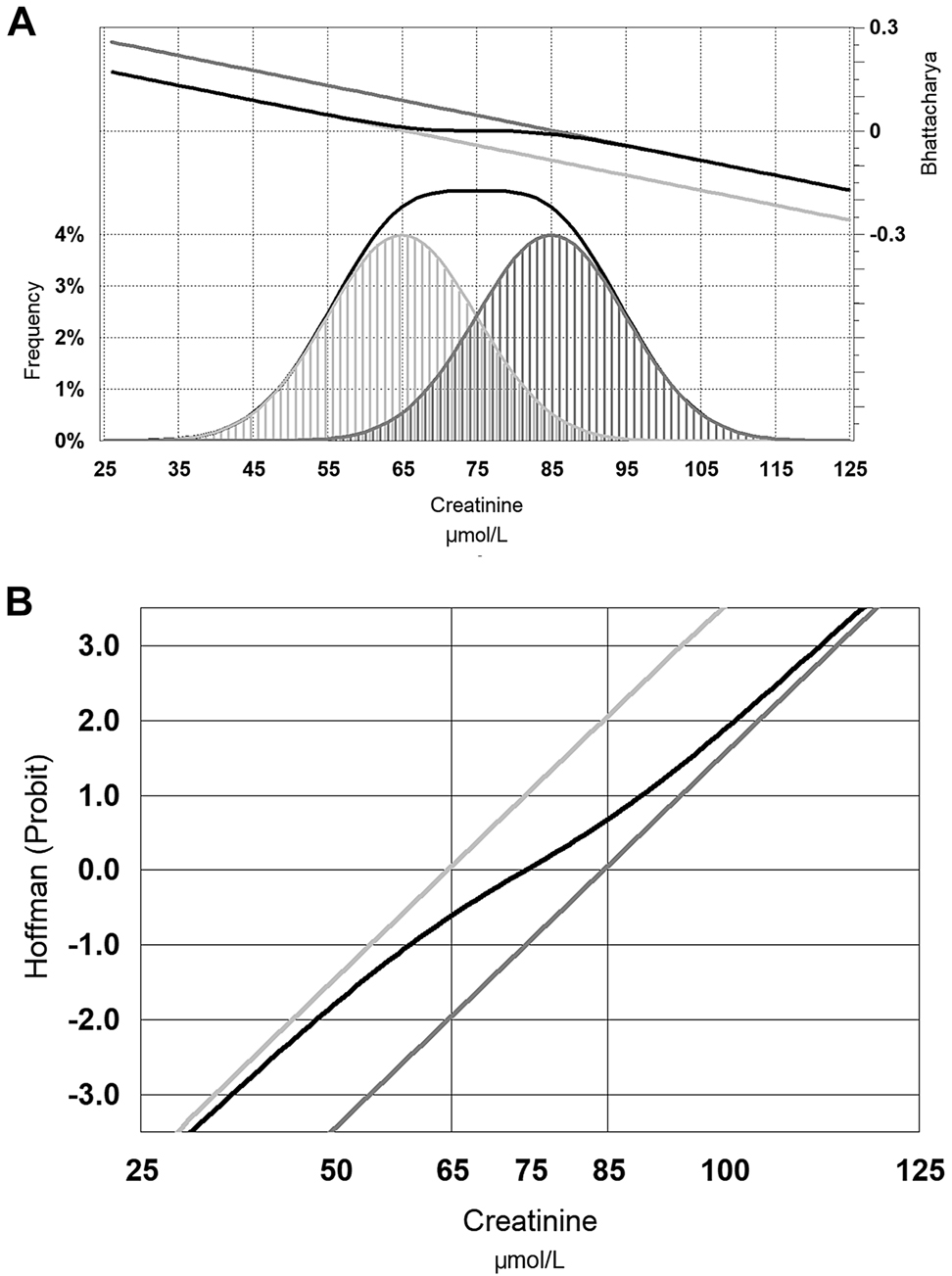
Hypothetical distribution of serum creatinine in men (dark grey), women (light grey) and the combined distribution of men and women (black line).
Panel (A) also shows the Bhattacharya function for each distribution and the combined distribution, while panel (B) shows the Hoffmann function (see text for further explanation).

Distribution of laboratory serum creatinine in young adults between 20 and 29 years of age; men (dark grey), women (light grey) and the combined distribution of men and women (black line).
Panel (A) also shows the Bhattacharya function for each distribution and the combined distribution, while panel (B) shows the Hoffmann function (see text for further explanation).
The Hoffmann technique is therefore usually simplistic and relies heavily on the initial exclusion of overlapping distributions. This is not always appreciated and modified Hoffmann techniques are often misused [63], and can be demonstrated to be inferior to the alternative common technique of deriving the underlying distribution – the Bhattacharya method [64].
Bhattacharya described a statistical approach of resolving a distribution into its Gaussian components in 1967 [65] by recognising that the slope of a Gaussian distribution (from left to right) rises but soon gradually falls toward zero slope at the zenith, then becomes increasingly negative before it dwindles away. The slope changes logarithmically, so the logarithm of the slope forms a straight line – as long as that distribution is not interfered with by an overlapping distribution. Figure 4A also includes the Bhattacharya line for the hypothetical male and female serum creatinine distributions, and show that the Bhattacharya line is the same for the combined distribution as the individual distribution when there is negligible overlap. Figure 5A shows the Bhattacharya lines for the real serum creatinine data, and shows how the Bhattacharya line for the combined distribution overlaps with the individual distributions where the overlap is negligible. The slope of the Bhattacharya line again correlates with the standard deviation of the slope, but the mean is the point at which the slope function would be zero. The selection of this linear portion of the line can be subjective, however objective statistical approaches can be applied [66].
One of the limitations of the Hoffmann and Bhattacharya methods, to date, is that while the correlation coefficient of the line of best fit provides a statistical measure of confidence in the proposed distribution, a routine method of estimating the confidence in the reference limits has not been published. A related challenge in the Bhattacharya method is the subjective choice of bin size and location for the frequency histogram which may influence the final result. This is particularly an issue when data has been rounded and/or transformed and to minimise both these issues, the data should start with as many significant figures as possible [67]. When large data sets are available, adjustment of the bin locations should not significantly affect the results.
The Bhattacharya technique was employed in clinical biochemistry within three years by Gindler [68] and refined by Baadenhuijsen and Smit in 1985 [69]. Online resources have been available [70], [71]. Because the Bhattacharya line is derived only from the unaffected part of the combined distribution, it is unaffected by outliers including the presence of disease, as long as unaffected linear part of the Bhattacharya line (which defines the reference population), represents at least 40% of the total population [67]. It is therefore useful to apply clinical exclusion techniques before using Bhattacharya for most analytes to increase the proportion of the combined distribution that represents the reference population.
If a distribution is close to symmetrical, it is generally true that the centre (mode) of the observed indirect distribution will be the mean. In any case, the possibility of overlapping populations increase as you move away from either of these central measures. This also depends on whether disease causes an increase or decrease. If disease causes increases e.g. alanine transaminase (ALT), then the lower side of the distribution is largely unaffected and the reference distribution can be estimated using results in the lower side of the distribution. Conversely, if disease generally causes lower results (e.g. Hb), then the upper part of the distribution can be used to estimate the underlying reference distribution. This is essentially the basis of the Pryce method [72]. The more challenging situation is when disease causes both increases and decreases (e.g. serum sodium), so we lose confidence as we move in either direction from the mode. Despite the relatively high frequency of results around the centre of the distribution, an increased reliance on this narrow span of data, is what usually makes it necessary to have large databases.
Advances in indirect reference interval estimation does not necessarily assume that the truncated central part of the distribution is unaffected by disease [73]. The ‘truncated minimum chi-square’ (TMC) approach starts with a Hoffmann estimate from this part of this distribution, then uses an iterative approach to define an assumed power normal distribution (including Box–Cox adjustment) using the data both within and outside the apparently unaffected interval [74].
I’ve been fortunate to work in ‘mega’ laboratories testing over 10,000 patients per day, which have access to very large databases. These private laboratories focus on primary healthcare and have provided the opportunity to define many indirect reference intervals from tumour markers [75], [76], [77], [78], hormones [79] to routine biochemistry [80], [81], [82] and routine haematology [83]. In my experience, using these very large databases, clinical exclusion is not as important as statistical exclusion because I use a statistical technique (Bhattacharya) that is least affected by outliers and overlapping disease populations. Others have also concluded that some indirect methods can work well in unselected populations [84].
Table 1 compares the clinical and statistical approaches to separating health and disease. The clinical approach is attractive to those that are clinically focussed and sceptical about how statistical methods might be able to separate subpopulations. The clinical approach does rely on the availability clinical information as well as an understanding of the effect of disease(s) on each laboratory test. The statistical approach can be applied to laboratory data without clinical information of understanding, however the complex statistical methods usually require very large databases to locate the small span of data unaffected by disease. While I personally prefer a combined approach, this requires both very large databases as well as a demonstrated consideration of available clinical information. I find the extra effort useful as it specifically quantifies the pathological impact of disease (which may not be known) at the same time as considering the relative impact of human physiology. In simpler terms, I can demonstrate that young adults have less disease, at the same time as demonstrating they are physiologically different to the elderly.
Comparison of clinical and statistical approaches to separating healthy and diseased populations using indirect reference interval methodologies.
| Clinical approach | Statistical approach | Combined approach | |
|---|---|---|---|
| Pre-requisites | Identify significant pre-analytical variations in the data. Identify significant analytical variations in the data. Identify physiological partitions for each test. | ||
| Advantages | Satisfies those that are sceptical about statistical approach. | Can be applied by most laboratories. | Satisfies statistical sceptics. Can be applied by most laboratories. |
| Disadvantages | Understand effect of disease(s) on test. | Complex statistical methods requiring large databases. | Understand effect of disease(s) on test. Complex statistical methods requiring large databases. |
Overlap and skewness due to overlap of healthy partitions
Just as importantly, a heterogeneous distribution may comprise overlapping partitions of healthy individuals described by physiological variations. Figure 6 shows that the skewed distribution for serum bilirubin could be interpreted as a logarithmic Gaussian distribution or a series of overlapping normal Gaussian population. The latter is more likely given that overlapping bilirubin distributions more appropriately reflect the common and distinct genetic polymorphisms in the UGT1A1 promoter [85]. It is highly desirable not to broaden reference intervals by ignoring important physiological distinctions as this may undermine the primary purpose (specificity) of reference intervals and in the case of serum bilirubin, this will lead to incorporation of Gilbert’s syndrome into the common reference interval. While it could be argued that this may be appropriate, it should be done consciously rather than accidentally.
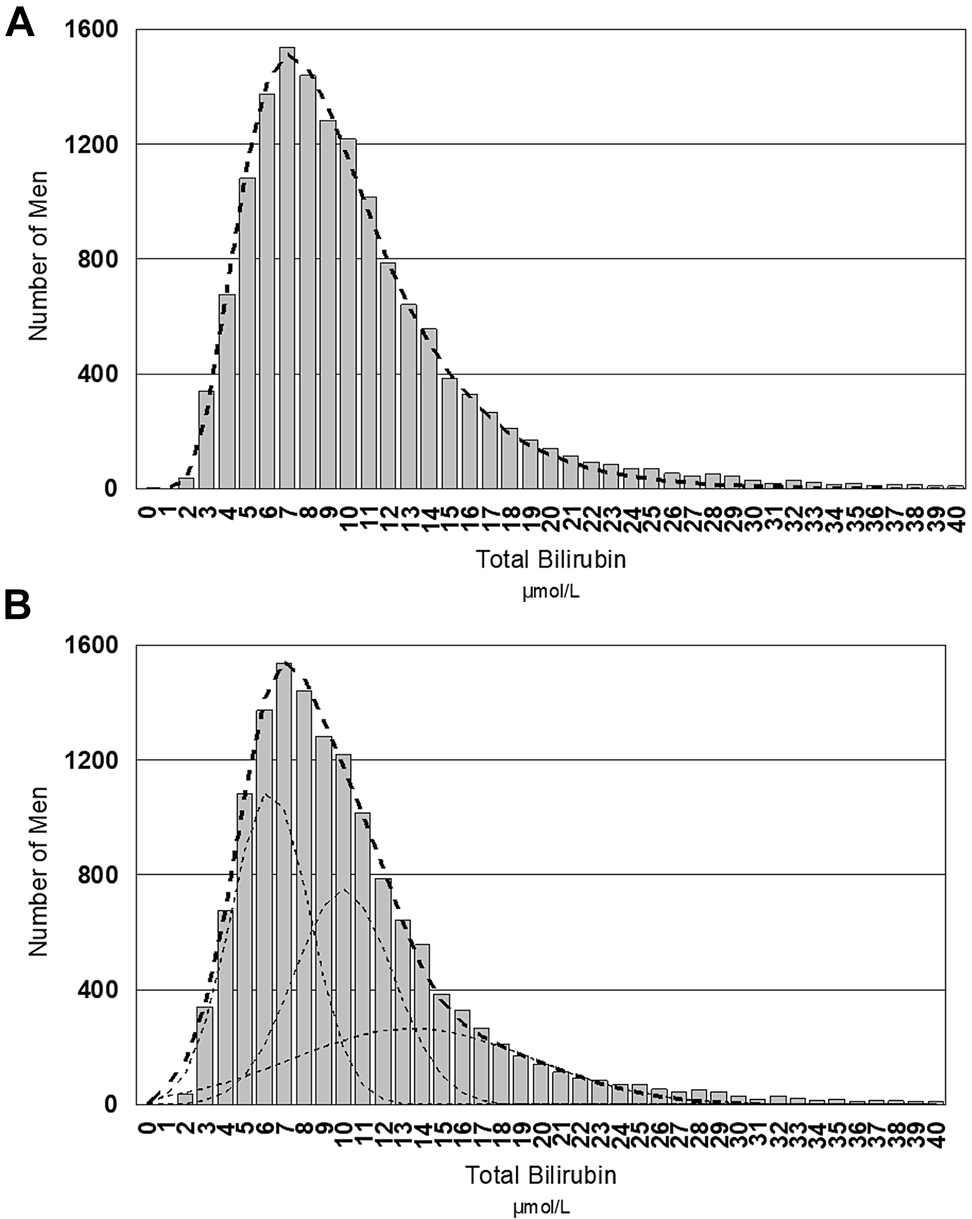
Distribution of serum bilirubin values in young men between 20 and 29 years of age.
Panel (A) shows the log Gaussian solution to the skewed distribution whilst panel (B) shows three overlapping normal Gaussian populations as the solution to the distribution.
Investigating partitioning can be just as relevant as generating the reference interval in the first place [86]. In my experience, overlap and skewness due to physiological heterogeneity is a more pressing issue than overlap or skewness due to disease and indirect reference interval techniques are a convenient tool for exploring physiological variations. Understanding physiology is therefore a pre-requisite to understanding reference interval partitioning [87] and the prevalence of physiological subgroups in the reference population should be known and observed in the calculations for every reference interval study [88]. There are very few (if any) measurands that are the naturally same across childhood and adulthood let alone gender and pregnancy. Concordet et al. [89] have indicated that complex techniques have several weakness, including separating young and old individuals rather than healthy and diseased ones. If indirect reference intervals are determined that do not demonstrate known physiological changes, then be very cautious about accepting that the investigators have accounted for the overlap due to disease.
Sometimes the differences between healthy groups seem small and a decision needs to be made about whether the difference is significant enough to justify a new partition. Clinical justification of partitioning should be related to the potential change in clinical specificity of the derived reference limits. Normally, a 95% reference interval will have a 2.5% false positive rate above the 97.5th centile and 2.5% false positive rate below the 2.5th centile. Harris and Boyd developed a statistical method for identifying partitions but observed that abnormal rates of less than 1.0%, or greater than 4.0%, deviate too much from the ideal value of 2.5% [90]. Lahti et al. [91] have more stringently determined that if more than 4.4% are flagging (rather than 2.5%), this justifies a new partition. Conversely if less than 3.3% are flagging, then partitions should be combined because the flag rate is not confidently different from 2.5%.
Partitioning related to pregnancy
Virtually all serum measurements in pregnancy are lower (due to haemodilution), except for the unique hormonal and placental products of pregnancy. Whilst it is relatively easy to partition children when calculating adult reference limits, it is not as easy to partition pregnancy because (i) the laboratory may not be informed the patient is pregnant, (ii) the patient may not realise they are pregnant and, most importantly, (iii) many Laboratory Information Systems lack the ability to store the gestational status or gestational age of the women they do know are pregnant. Nevertheless, laboratories can identify pregnant individuals by using commonly co-requested tests [92] such as Rubella testing, maternal serum screening (which may have information on gestational age and race) or gestational diabetes testing (which may also have gestational age and provide gestational diabetes status).
The proportion of young women that are pregnant will vary from laboratory to laboratory, so if the proportion is low, the impact on the overall distribution may be minimised. Nevertheless it is important to have an estimate of how large that proportion is if you want to be confident that the indirect reference limits you calculate for non-pregnant young women aren’t biased by the pregnancy subgroup.
Identifying that women are pregnant is only half the problem, as many reference limits change with gestational age, and even the conventions regarding the definitions of the arbitrary three trimesters becomes important [93]. As an example, a patient or doctor may claim a woman is ‘one week pregnant’, but this is technically impossible as logically the woman hasn’t even ovulated a week after her last menstrual period. Unfortunately nature doesn’t follow societal conventions and analytes may change significantly within one of the trimesters, such as for Thyroid Stimulating Hormone (TSH), where TSH levels are much lower in the last part of the first trimester (when the thyrotropic effects of human Chorionic Gonadotrophin (hCG) are maximal) [94]. While it is commonly understood that release of placental alkaline phosphatase (ALP) causes a marked elevation in serum ALP in pregnancy, it is not as commonly understood that serum ALP is lower than in non-pregnant women in the first trimester (due to haemodilution), and the placental increase in ALP only starts to become evident late in the second trimester [95].
Partitioning childhood
The difficult issues of recruiting and consent for obtaining samples for direct reference intervals is obviated using indirect approaches. Another difficulty in ‘childhood’ is that children are continually developing and newborns, infants, toddlers, primary and secondary children, all vary in their physiological stages in development. This makes it difficult to know where to draw the line for partitioning, and some analytes change continuously from childhood to puberty e.g. rising creatinine (representing muscular development) and rising and falling ALP (representing the changes in bone development) [96].
The benefit of larger indirect reference interval databases is that the paediatric changes can be explored by plotting the test median against age, and continuous reference limits can be defined. Most Laboratory Information Systems depend on discrete partitioning based on age. Age may be unreliable because it does not always describe the stage of development for any child with puberty illustrating this challenge when children reach ‘Tanner Stages’ of pubertal development at differing ages. While the end of puberty could be assigned adult status, this will also vary from individual to individual. In general terms, the default ages of 16 years for girls and 18 years for boys typically represent physiological adulthood but some analytes e.g., ALP, may continue to be mildly elevated in young men until the age of 21. I was recently surprised to find that free tri-iodothyronine (fT3) falls after age 16 in girls and a few years later in boys (unpublished data), and whilst this could be either an area of unappreciated physiology, or one of the many artifacts of analogue free hormone measurement, it is clinically important to appreciate when reporting.
Partitioning the elderly
It may be conventional to define elderly as someone over the age of 65 years, and indeed, it seems that many measurands rise from about this age. Without getting into the many theories of ageing, geriatrics (like paediatrics) is not a single physiological state, but one that continuously changes (unfortunately deteriorating), and 65 year olds can significant differ from 75, 85 or 95 year olds.
The increased prevalence of disease in the elderly adds to the challenge of partitioning by age and even indirect reference interval studies can have difficulty accumulating enough data to sufficiently partition the large changes that occur with ageing [97]. Troponin T and homocysteine levels are dependent on renal excretion, but even when excluding elderly patients with renal impairment from the data set, a rise with ageing is still seen, which correlates with risk.
Conclusions
While direct reference intervals should be preferred, they have several limitations. They seldom account for all the major pre-analytical factors that affect test results such as age, gender and ethnicity let alone the minor factors such as diet, exercise, smoking, drugs of abuse including alcohol and medications [98]. Furthermore, methods vary between manufacturers and any analytical improvements also require reassessment of the appropriateness of previously defined direct reference limit.
The indirect approach can address the very difficult partitions across paediatrics, pregnancy and the elderly where direct reference intervals have even greater complexity and cost. The indirect approach is not only convenient and cheap but also operates on data from the ‘real world’ of clinical practice. The pre-analytical factors of collection and transport in the reference population match routine processing. Reference intervals should be derived from a reference population as close as possible to the populations being assessed [99] and patient traits including e.g. diet and exercise should be similar to the reference population [100]. A patient’s comorbidities (e.g. obesity) might be present in the reference population [101]. Perhaps hospitalized patients, who are generally stressed and supine, be interpreted against reference intervals developed from healthy ambulatory populations or against unaffected hospitalised patients [28]. These often poorly defined case mix factors are considered to be flaws of the indirect reference interval approach [102], but I would agree with Barth that these are significant advantages [102].
Summary
Indirect reference intervals are cheap and convenient and can address the many aspects of reference interval derivation that are hard to address with expensive direct reference interval studies. The two principles of clinical exclusion of diseased individuals from the reference population, combined with statistical identification of overlapping populations and outliers must always be considered. The use of advanced statistical techniques that focus on the dominant reference population, and are least affected by the presence of overlapping populations, may be more important than clinical exclusion. The value of indirect reference intervals should be demonstrated by their ability to identify the numerous physiological variations already present in laboratory data, that direct reference intervals seldom accommodate.
-
Research funding: None declared.
-
Author contributions: The author has accepted responsibility for the entire content of this manuscript and approved its submission.
-
Competing interests: The author states no conflict of interest.
References
1. Özarda, Y, Sikaris, K, Streichert, T, Macri, J, on behalf of IFCC-Committee on Reference Intervals and Decision Limits (C-RIDL). Distinguishing reference intervals and clinical decision limits – a review by the IFCC committee on reference intervals and decision limits. Crit Rev Clin Lab Sci 2018;55:420–31. https://doi.org/10.1080/10408363.2018.1482256.Search in Google Scholar PubMed
2. Jones, GRD, Haeckel, R, Loh, TP, Sikaris, K, Streichert, T, Katayev, A, et al.. IFCC Committee on Reference Intervals and Decision Limits. Indirect methods for reference interval determination – review and recommendations. Clin Chem Lab Med 2018;57:20–9. https://doi.org/10.1515/cclm-2018-0073.Search in Google Scholar PubMed
3. Cembrowski, GS, Chan, J, Zhang, MM. Third NHANES used to create comprehensive health-associated reference intervals for 21 serum chemistry analytes measured by the Hitachi 737. Clin Chem 2001;27:A118.Search in Google Scholar
4. Cheng, CK, Chan, J, Cembrowski, GS, van Assendeift, OW. Complete blood count reference interval diagrams derived from NHANES III: stratification by age, sex, race. Lab Hematol 2004;10:42–53. https://doi.org/10.1532/lh96.04010.Search in Google Scholar PubMed
5. Fulgoni, VL3rd, Agarwal, S, Kellogg, MD, Lieberman, HR. Establishing pediatric and adult RBC reference intervals with NHANES data using piecewise regression. Am J Clin Pathol 2019;151:128–42. https://doi.org/10.1093/ajcp/aqy116.Search in Google Scholar PubMed PubMed Central
6. CLSI EP28-A3C. Defining, establishing, and verifying reference intervals in the clinical laboratory, 3rd ed. Wayne, PA, USA: Clinical & Laboratory Standards Institute; 2010.Search in Google Scholar
7. Dankner, R, Boffetta, P, Keinan-Boker, L, Balicer, RD, Berlin, A, Olmer, L, et al.. Diabetes, prostate cancer screening and risk of low- and high-grade prostate cancer: an 11 year historical population follow-up study of more than 1 million men. Diabetologia 2016;59:1683–91. https://doi.org/10.1007/s00125-016-3972-x.Search in Google Scholar PubMed PubMed Central
8. Gapstur, SM, Gann, PH, Colangelo, LA, Barron-Simpson, R, Kopp, P, Dyer, A, et al.. Postload plasma glucose concentration and 27-year prostate cancer mortality. Cancer Causes Control 2001;12:763–72. https://doi.org/10.1023/a:1011279907108.10.1023/A:1011279907108Search in Google Scholar
9. Sikaris, KA, McLachlan, RI, Kazlauskas, R, de Kretser, D, Holden, CA, Handelsman, DJ. Reproductive hormone reference intervals for healthy fertile young men: evaluation of automated platform assays. J Clin Endocrinol Metab 2005;90:5928–36. https://doi.org/10.1210/jc.2005-0962.Search in Google Scholar PubMed
10. Farrell, CJ, Nguyen, L. Indirect reference intervals: harnessing the power of stored laboratory data. Clin Biochem Rev 2019;40:99–111.10.33176/AACB-19-00022Search in Google Scholar
11. Miller, WG, Chinchilli, VM, Gruemer, HD, Nance, WE. Sampling from a skewed population distribution as exemplified by estimation of the creatine kinase upper reference limit. Clin Chem 1984;30:18–23. https://doi.org/10.1093/clinchem/30.1.18.Search in Google Scholar
12. Sikaris, KA, Kanowski, D, Ward, G, Lu, Z. Seasonal effect on the laboratory prevalence of Vitamin D deficiency across Australia. Clin Biochem Rev 2009;30:S19.Search in Google Scholar
13. Higgins, T, Saw, S, Sikaris, KA, Wiley, CL, Cembrowski, G, Lyon, AW, et al.. Seasonal variation in hemoglobin A1c: is it the same in both hemispheres? J Diabetes Sci Technol 2009;3:668–71. https://doi.org/10.1177/193229680900300408.Search in Google Scholar PubMed PubMed Central
14. Dalpino, F, Menna-Barreto, K, Castilho, L, De Faria, E. Biological rhythms of biochemical serum parameters in a Brazilian population: a three-year study. Chronobiol Int 2005;22:925–35. https://doi.org/10.1080/07420520500263052.Search in Google Scholar PubMed
15. Özçürümez, MK, Haeckel, R. Biological variables influencing the estimation of reference limits. Scand J Clin Lab Invest 2018;78:337–45. https://doi.org/10.1080/00365513.2018.1471617.Search in Google Scholar PubMed
16. Botros, M, Lu, ZX, McNeil, AM, Sikaris, KA. Clinical notes as indicators for vitamin B12 levels via test data mining. Pathology 2014;46:S84. https://doi.org/10.1097/01.pat.0000443628.07829.70.Search in Google Scholar
17. Sikaris, KA, Trambas, C, Yen, T, Lu, ZX. Appropriateness of pathology requests according clinical notes supplied with ferritin requests using the metric of mean abnormality rate. Clin Biochem Rev 2018;39:S22.Search in Google Scholar
18. Lu, ZX, Taylor, N, Caldwell, G, Wu, J, Trambas, CM, Yen, T, et al.. Establishing population and gestational age specific TFT reference intervals for the Abbott method using local data mining. Pathology 2018;50:S92. https://doi.org/10.1016/j.pathol.2017.12.255.Search in Google Scholar
19. Lu, ZX, Trambas, C, Yen, T, Sikaris, KA. Establishing population and gestational age specific TFT reference intervals for the Roche method using local data mining. Pathology 2018;50(S1):S92–3.10.1016/j.pathol.2017.12.255Search in Google Scholar
20. Vadiveloo, T, Donnan, PT, Murphy, MJ, Leese, GP. Age and gender-specific TSH reference intervals in people with no obvious thyroid disease in Tayside, Scotland: the Thyroid Epidemiology, Audit, and Research Study (TEARS). J Clin Endocrinol Metab 2013;98:1147–53. https://doi.org/10.1210/jc.2012-3191.Search in Google Scholar PubMed
21. Bonney, A, Mayne, DJ, Jones, BD, Bott, L, Andersen, SEJ, Caputi, P, et al.. Area-level socioeconomic gradients in overweight and obesity in a community-derived cohort of health service users – a cross-sectional study. PLoS One 2015;10:e0137261. https://doi.org/10.1371/journal.pone.0137261.Search in Google Scholar PubMed PubMed Central
22. Cembrowski, GS, Chan, J. Stratification of health-related reference intervals for ALT, GGT, AST, ALP, LD by waist circumference: an aid for weight reduction? Clin Chem 2002;48:A38–9.Search in Google Scholar
23. Xia, L, Chen, M, Liu, M, Tao, Z, Li, S, Wang, L, et al.. Nationwide multicenter reference interval study for 28 common biochemical analytes in China. Medicine (Baltim) 2016;95:e2915. https://doi.org/10.1097/md.0000000000002915.Search in Google Scholar
24. Koerbin, G, Cavanaugh, JA, Potter, JM, Abhayaratna, WP, West, NP, Glasgow, N, et al.. ‘Aussie normals’: an a priori study to develop clinical chemistry reference intervals in a healthy Australian population. Pathology 2015;47:138–44. https://doi.org/10.1097/pat.0000000000000227.Search in Google Scholar PubMed
25. Ichihara, K, Özarda, Y, Barth, JH, Klee, G, Shimizu, Y, Xia, L, et al.. A global multicenter study on reference values: 2. Exploration of sources of variation across the countries. Clin Chim Acta 2017;464:83–97. https://doi.org/10.1016/j.cca.2016.09.015.Search in Google Scholar PubMed
26. Sikaris, KA. Weighing up our clinical confidence in reference limits. Clin Chem 2020;66:1475–6. https://doi.org/10.1093/clinchem/hvaa230.Search in Google Scholar PubMed
27. Kouri, T, Kairisto, V, Virtanen, A, Uusipaikka, E, Rajamäki, A, Finneman, H, et al.. Reference intervals developed from data for hospitalized patients: computerized method based on combination of laboratory and diagnostic data. Clin Chem 1994;40:2209–15. https://doi.org/10.1093/clinchem/40.12.2209.Search in Google Scholar
28. Cembrowski, GS, Fairbanks, VF. Can hematology reference intervals be derived from hospitalized patients’ data? Clin Chem 1995;41:1048–50. https://doi.org/10.1093/clinchem/41.7.1048.Search in Google Scholar
29. Poole, S, Schroeder, LF, Shah, N. An unsupervised learning method to identify reference intervals from a clinical database. J Biomed Inf 2016;59:276–84. https://doi.org/10.1016/j.jbi.2015.12.010.Search in Google Scholar PubMed PubMed Central
30. Pivovarov, R, Albers, DJ, Sepulveda, JL, Elhadad, N. Identifying and mitigating biases in EHR laboratory tests. J Biomed Inf 2014;51:24–34. https://doi.org/10.1016/j.jbi.2014.03.016.Search in Google Scholar PubMed PubMed Central
31. Bock, BJ, Dolan, CT, Miller, GC, Fitter, WF, Hartsell, BD, Crowson, AN, et al.. The data warehouse as a foundation for population-based reference intervals. Am J Clin Pathol 2003;120:662–70. https://doi.org/10.1309/w8j85ag4wdg6jgj9.Search in Google Scholar
32. Krøll, J, Saxtrup, O. On the use of patient data for the definition of reference intervals in clinical chemistry. Scand J Clin Lab Invest 1998;58:469–73.10.1080/00365519850186265Search in Google Scholar PubMed
33. Giavarina, D, Dorizzi, RM, Soffiati, G. Indirect methods for reference intervals based on current data. Clin Chem 2006;52:335–7. https://doi.org/10.1373/clinchem.2005.062182.Search in Google Scholar PubMed
34. Farrell, CL, Nguyen, L, Carter, AC. Parathyroid hormone: data mining for age-related reference intervals in adults. Clin Endocrinol 2018;88:311–7. https://doi.org/10.1111/cen.13486.Search in Google Scholar PubMed
35. Grossi, E, Colombo, R, Cavuto, S, Franzini, C. The REALAB project: a new method for the formulation of reference intervals based on current data. Clin Chem 2005;51:1232–40. https://doi.org/10.1373/clinchem.2005.047787.Search in Google Scholar PubMed
36. Weber, GM, Kohane, IS. Extracting physician group intelligence from electronic health records to support evidence based medicine. PLoS One 2013;8:e64933. https://doi.org/10.1371/journal.pone.0064933.Search in Google Scholar PubMed PubMed Central
37. Sikaris, KA. Biochemistry on the human scale. Clin Biochem Rev 2010;31:121–8.Search in Google Scholar
38. Fraser, CG. Biological variation: from principles to practice. Washington, DC: AACC Press; 2001.Search in Google Scholar
39. Quetelet, A. A treatise on man and the development of his faculties (Reprinted 1842). New York, USA: Burt Franklin; 1968.Search in Google Scholar
40. Hyltoft Petersen, P, Blaabjerg, O, Andersen, M, Jørgensen, LG, Schousboe, K, Jensen, E. Graphical interpretation of confidence curves in rankit plots. Clin Chem Lab Med 2004;42:715–24. https://doi.org/10.1515/cclm.2004.122.Search in Google Scholar
41. Jensen, E, Hyltoft Petersen, P, Blaabjerg, O, Hansen, PS, Brix, TH, Kyvik, KH, et al.. Establishment of a serum thyroid stimulating hormone (TSH) reference interval in healthy adults. The importance of environmental factors, including thyroid antibodies. Clin Chem Lab Med 2004;42:824–32. https://doi.org/10.1515/cclm.2004.136.Search in Google Scholar PubMed
42. Feng, C, Wang, H, Lu, N, Chen, T, He, H, Lu, Y, et al.. Logtransformation and its implications for data analysis. Shanghai Arch Psychiatry 2014;26:105–9. https://doi.org/10.3969/j.issn.1002-0829.2014.02.009.Search in Google Scholar PubMed PubMed Central
43. Boyd, JC, Lacher, DA. A multistage Gaussian transformation algorithm for clinical laboratory data. Clin Chem 1982;28:1735–41. https://doi.org/10.1093/clinchem/28.8.1735.Search in Google Scholar
44. Box, G, Cox, D. An analysis of transformations. J R Stat Soc Series B Stat Methodol 1964;26:211–52. https://doi.org/10.1111/j.2517-6161.1964.tb00553.x.Search in Google Scholar
45. Jones, GRD. Reference interval determination by Bhattacharya analysis on skewed distributions – problems and pitfalls. Clin Biochem Rev 2006;27:S34.Search in Google Scholar
46. Linnet, K. Two-stage transformation systems for normalization of reference distributions evaluated. Clin Chem 1987;33:381–6. https://doi.org/10.1093/clinchem/33.3.381.Search in Google Scholar
47. Cleophas, TJ, Zwinderman, AH. Gamma distribution for estimating the predictors of medical outcome scores (110 patients). In: Machine learning in medicine – a complete overview. Springer, Cham; 2015.10.1007/978-3-319-15195-3_80Search in Google Scholar
48. Vos, M, Joost van Pelt, L, Kok, MB, Dijck-Brouwer, DAJ, Heiner-Fokkema, MR, Dikkeschei, LD, et al.. Folate reference interval estimation in the Dutch general population. Pract Lab Med 2019;16:e00127. https://doi.org/10.1016/j.plabm.2019.e00127.Search in Google Scholar PubMed PubMed Central
49. Brinkworth, RSA, Whitham, E, Nazeran, H. Establishment of paediatric biochemical reference intervals. Ann Clin Biochem 2004;41:321–9. https://doi.org/10.1258/0004563041201572.Search in Google Scholar PubMed
50. Shine, B. Use of routine clinical laboratory data to define reference intervals. Ann Clin Biochem 2008;45:467–75. https://doi.org/10.1258/acb.2008.008028.Search in Google Scholar PubMed
51. Dawodu, A, Agarwal, M, Hossain, M, Kochiyil, J, Zayed, R. Hypovitaminosis D and vitamin D deficiency in exclusively breast-feeding infants and their mothers in summer: a justification for vitamin D supplementation of breast-feeding infants. J Pediatr 2003;142:169–73. https://doi.org/10.1067/mpd.2003.63.Search in Google Scholar PubMed
52. Hepp, T, Zierk, J, Rauh, M, Metzler, M, Mayr, A. Latent class distributional regression for the estimation of non-linear reference limits from contaminated data sources. BMC Bioinf 2020;21:524. https://doi.org/10.1186/s12859-020-03853-3.Search in Google Scholar PubMed PubMed Central
53. Barnett, V, Lewis, T. Outliers in statistical data, 3rd ed. Chichester: J. Wiley and Sons; 1994.Search in Google Scholar
54. Dixon, WJ. Processing data for outliers. Biometrics 1953;9:74–89. https://doi.org/10.2307/3001634.Search in Google Scholar
55. Reed, AH, Henry, RJ, Manson, WB. Influence of statistical method used on the resulting estimate of normal range. Clin Chem 1971;17:275–84. https://doi.org/10.1093/clinchem/17.4.275.Search in Google Scholar
56. Tukey, JW. Exploratory data analysis. Reading, MA, USA: Addison-Wesley; 1977.Search in Google Scholar
57. Bjerner, J, Theodorsson, E, Hovig, E, Kallner, A. Non-parametric estimation of reference intervals in small non-Gaussian sample sets. Accred Qual Assur 2009;14:185–92. https://doi.org/10.1007/s00769-009-0490-2.Search in Google Scholar
58. Horn, PS, Feng, L, Li, Y, Pesce, AJ. Effect of outliers and nonhealthy individuals on reference interval estimation. Clin Chem 2001;47:2137–45. https://doi.org/10.1093/clinchem/47.12.2137.Search in Google Scholar
59. Solberg, HE, Lahti, A. Detection of outliers in reference distributions: performance of Horn’s algorithm. Clin Chem 2005;51:2326–32. https://doi.org/10.1373/clinchem.2005.058339.Search in Google Scholar PubMed
60. Hoffmann, RG. Statistics in the practice of medicine. JAMA 1963;185:864–73. https://doi.org/10.1001/jama.1963.03060110068020.Search in Google Scholar PubMed
61. Neumann, GJ. The determination of normal ranges from routine laboratory data. Clin Chem 1968;14:979–88. https://doi.org/10.1093/clinchem/14.10.979.Search in Google Scholar
62. Katayev, A, Fleming, JK, Luo, D, Fisher, AH, Sharp, TM. Reference intervals data mining: no longer a probability paper method. Am J Clin Pathol 2015;143:134–42. https://doi.org/10.1309/ajcpqprnib54wfkj.Search in Google Scholar
63. Holmes, DT, Buhr, KA. Widespread incorrect implementation of the Hoffmann method, the correct approach, and modern alternatives. Am J Clin Pathol 2019;151:328–36. https://doi.org/10.1093/ajcp/aqy149.Search in Google Scholar
64. Jones, GRD, Sikaris, KA. Statistical showdown – Hoffmann v Bhattacharya for data mining. Clin Biochem Rev 2016;37:S20.Search in Google Scholar
65. Bhattacharya, CG. A simple method of resolution of a distribution into Gaussian components. Biometrics 1967;23:115–35. https://doi.org/10.2307/2528285.Search in Google Scholar
66. Oosterhuis, WP, Modderman, TA, Pronk, C. Reference values: Bhattacharya or the method proposed by the IFCC? Ann Clin Biochem 1990;27:359–65. https://doi.org/10.1177/000456329002700413.Search in Google Scholar
67. Jones, GRD. Bhattacharya and bins – avoiding analysis pitfalls. Clin Biochem Rev 2019;40:S29.10.1002/9781119278207Search in Google Scholar
68. Gindler, EM. Calculation of normal ranges by methods used for the resolution of overlapping Gaussian distributions. Clin Chem 1970;16:124–8. https://doi.org/10.1093/clinchem/16.2.124.Search in Google Scholar
69. Baadenhuijsen, H, Smit, JC. Indirect estimation of clinical chemical reference intervals from total hospital patient data: application of a modified Bhattacharya procedure. J Clin Chem Clin Biochem 1985;23:829–39. https://doi.org/10.1515/cclm.1985.23.12.829.Search in Google Scholar
70. Jones, GR. Bhattacharya spreadsheet [Online]. Available from: http://www.sydpath.stvincents.com.au/index.htm [Accessed 5 Feb 2021].Search in Google Scholar
71. Chesher, D. Bellview: a tool to perform Bhattacharya analysis on laboratory data [Online]. Available from: https://sourceforge.net/projects/bellview/ [Accessed 5 Feb 2021].Search in Google Scholar
72. Pryce, JD. Level of haemoglobin in whole blood and red blood-cells, and proposed convention for defining normality. Lancet 1960;2:333–6. https://doi.org/10.1016/s0140-6736(60)91480-x.Search in Google Scholar
73. Arzideh, F, Wosniok, W, Gurr, E, Hinsch, W, Schumann, G, Weinstock, N, et al.. A plea for intra-laboratory reference limits. Part 2. A bimodal retrospective concept for determining reference limits from intra-laboratory databases demonstrated by catalytic activity concentrations of enzymes. Clin Chem Lab Med 2007;45:1043–57. https://doi.org/10.1515/cclm.2007.250.Search in Google Scholar PubMed
74. Wosniok, W, Haeckel, R. A new indirect estimation of reference intervals: truncated minimum chi-square (TMC) approach. Clin Chem Lab Med 2019;57:1933–47. https://doi.org/10.1515/cclm-2018-1341.Search in Google Scholar PubMed
75. Sikaris, KA, Stringer, M, Dennis, PM. Using patient data to validate age specific reference intervals for the Abbott IMx PSA assay. Clin Biochem Rev 1994;15:101.Search in Google Scholar
76. Sikaris, KA, Guerin, MD. Age-specific reference intervals for the Ciba-Corning ACS-180 PSA assay. Clin Biochem Rev 1994;15:102.Search in Google Scholar
77. Sikaris, KA, Caldwell, G. Age related reference intervals for the Architect PSA. Clin Biochem Rev 2007;28:S33.Search in Google Scholar
78. Sikaris, KA, Lu, Z, Greco, S, Kanowski, D, Freemantle, M, Yen, T, et al.. Highly specific reference intervals for CA125II assays. Clin Biochem Rev 2009;30:S21.Search in Google Scholar
79. Sikaris, KA, Wootton, R, Mitchell, DK, Meerkin, M, Taylor, N, Gay, S. TSH reference intervals for the ACS:180 defined from patient data. Clin Biochem Rev 1999;20:90.Search in Google Scholar
80. Taylor, N, Meerkin, M, Sikaris, KA, McNeil, A, Garcia Webb, P, Guerin, M. Patient data defined LFT reference intervals. Clin Biochem Rev 2001;22:89.Search in Google Scholar
81. Sikaris, KA, Kanowski, D, Caldwell, G, Sack, S, Flatman, R. Consensus network reference intervals. Clin Biochem Rev 2006;27:S34.Search in Google Scholar
82. Sikaris, KA, Lu, Z, Kanowski, D, Price, L, Flatman, R, Caldwell, G, et al.. Defining Sonic network reference intervals for children. Clin Biochem Rev 2009;30:S20.Search in Google Scholar
83. Robotham, B, Maxwell, E, Sikaris, KA. Indirect estimation of haematology reference intervals by data mining. Int J Lab Hematol 2010;32:90.Search in Google Scholar
84. Naus, AJ, Borst, A, Kuppens, PS. The use of patient data for the calculation of reference values for some haematological parameters. J Clin Chem Clin Biochem 1980;18:621–5. https://doi.org/10.1515/cclm.1980.18.10.621.Search in Google Scholar PubMed
85. Erlinger, S, Arias, IM, Dhumeaux, D. Inherited disorders of bilirubin transport and conjugation: new insights into molecular mechanisms and consequences. Gastroenterology 2014;146:1625–38. https://doi.org/10.1053/j.gastro.2014.03.047.Search in Google Scholar PubMed
86. Kjelgard-Hansen, M. Stay afloat in the tsunami: a focus on clinical relevance when partitioning reference intervals. Vet J 2010;185:245–6.10.1016/j.tvjl.2009.08.015Search in Google Scholar PubMed
87. Sikaris, KA. The physiology of reference intervals. Clin Biochem Rev 2014;35:3–14.Search in Google Scholar
88. Lahti, A, Hyltoft Petersen, P, Boyd, JC. Impact of subgroup prevalences on partitioning of Gaussian-distributed reference values. Clin Chem 2002;48:1987–99. https://doi.org/10.1093/clinchem/48.11.1987.Search in Google Scholar
89. Concordet, D, Geffré, A, Braun, JP, Trumel, C. A new approach for the determination of reference intervals from hospital-based data. Clin Chim Acta 2009;405:43–8. https://doi.org/10.1016/j.cca.2009.03.057.Search in Google Scholar PubMed
90. Harris, EK, Boyd, JC. On dividing reference data into subgroups to produce separate reference ranges. Clin Chem 1990;36:265–70. https://doi.org/10.1093/clinchem/36.2.265.Search in Google Scholar
91. Lahti, A, Hyltoft Petersen, P, Boyd, JC, Fraser, CG, Jørgensen, N. Objective criteria for partitioning Gaussian distributed reference values into subgroups. Clin Chem 2002;48:338–52. https://doi.org/10.1093/clinchem/48.2.338.Search in Google Scholar
92. Blatt, AJ, Nakamoto, JM, Kaufman, HW. National status of testing for hypothyroidism during pregnancy and postpartum. Clin Endocrinol Metabol 2012;97:777–84. https://doi.org/10.1210/jc.2011-2038.Search in Google Scholar PubMed
93. Hadlow, N, Sikaris, K. Aspects to consider in adopting pregnancy-specific reference intervals. Clin Biochem Rev 2015;36:127–32.Search in Google Scholar
94. Laurberg, P, Andersen, SL, Hindersson, P, Nohr, EA, Olsen, J. Dynamics and predictors of serum TSH and fT4 reference limits in early pregnancy: a study within the Danish national birth cohort. J Clin Endocrinol Metab 2016;101:2484–92. https://doi.org/10.1210/jc.2016-1387.Search in Google Scholar PubMed
95. Ekinci, E, Lu, ZX, Sikaris, KA, Atanasovski, D, Bittar, I, Lam, Q, et al.. Alkaline phosphatase reference intervals in pregnancy. Clin Biochem Rev 2012;33:S23.Search in Google Scholar
96. Hoq, M, Matthews, S, Karlaftis, V, Burgess, J, Cowley, J, Donath, S, et al.. Reference values for 30 common biochemistry analytes across 5 different analysers in neonates and children 30 Days to 18 Years of age. Clin Chem 2019;65:1317–26. https://doi.org/10.1373/clinchem.2019.306431.Search in Google Scholar PubMed
97. Özarda, Y, Aslan, D. Use of total patient data for indirect estimation of reference intervals for 40 clinical chemical analytes in Turkey. Clin Chem Lab Med 2006;44:867–76.10.1515/CCLM.2006.139Search in Google Scholar
98. Ritchie, RF, Palomaki, G. Selecting clinically relevant populations for reference intervals. Clin Chem Lab Med 2004;42:702–9. https://doi.org/10.1515/cclm.2004.120.Search in Google Scholar
99. Solberg, HE, Gräsbeck, R. Reference values. Adv Clin Chem 1989;27:1–79. https://doi.org/10.1016/s0065-2423(08)60181-x.Search in Google Scholar
100. Ceriotti, F, Hinzmann, R, Panteghini, M. Reference intervals: the way forward. Ann Clin Biochem 2009;46:8–17. https://doi.org/10.1258/acb.2008.008170.Search in Google Scholar PubMed
101. Solberg, HE. Using a hospitalized population to establish reference intervals: pros and cons. Clin Chem 1994;40:2205–6. https://doi.org/10.1093/clinchem/40.12.2205.Search in Google Scholar
102. Barth, JH. Reference ranges still need further clarity. Ann Clin Biochem 2009;46:1–2. https://doi.org/10.1258/acb.2008.008187.Search in Google Scholar PubMed
© 2021 Kenneth A. Sikaris, published by De Gruyter, Berlin/Boston
This work is licensed under the Creative Commons Attribution 4.0 International License.
Articles in the same Issue
- Frontmatter
- Editorial
- Indirect approaches to estimate reference intervals
- Reviews
- Review of potentials and limitations of indirect approaches for estimating reference limits/intervals of quantitative procedures in laboratory medicine
- Separating disease and health for indirect reference intervals
- Opinion Papers
- Functional reference limits: a case study of serum ferritin
- Application of the TML method to big data analytics and reference interval harmonization
- Reference limits of high-sensitive cardiac troponin T indirectly estimated by a new approach applying data mining. A special example for measurands with a relatively high percentage of values at or below the detection limit
- Age and sex dependent reference intervals for random plasma/serum glucose concentrations related to different sampling devices and determined by an indirect procedure with data mining
- Original Articles
- Indirect estimation of reference intervals using first or last results and results from patients without repeated measurements
- The influence of sampling time on indirect reference limits, decision limits, and the estimation of biological variation of random plasma glucose concentrations
- Short Communications
- Diurnal variation of leukocyte counts affects the indirect estimation of reference intervals
- Reference intervals for platelet indices in seniors and frequency of abnormal results in a population-based setting: a comparison between directly and indirectly estimated reference intervals
- Calculation of indirect reference intervals of plasma lipase activity of adults from existing laboratory data based on the Reference Limit Estimator integrated in the OPUS::L information system