Equivalence limits of reference intervals for partitioning of population data. Relevant differences of reference limits
-
Rainer Haeckel
 ,
Werner Wosniok
,
Werner Wosniok

Abstract:
Reference limits need to be compared with each other for two main purposes: to evaluate the clinical relevance of a possible difference, if limits are obtained from the same population but at different time periods, or to check if limits derived from two different subpopulations can be considered as identical. The comparison of reference limits required for the periodic reviewing of applied reference limits and for checking the transferability of reference limits adopted from external sources according to international standards is an example for the first case. In the second case, a decision is intended whether the full population has to be partitioned (stratified) into the subpopulations under consideration (e.g. males and females). In both situations, differences may be due either to analytical errors, to biological differences or to both effects. The difference between reference limits may be acceptable if it is within permissible limits. For establishing permissible limits, the concept of equivalence limits was adopted to assess the relevance of differences between two reference limits. The concept bases on the permissible uncertainty at a particular reference limit. The permissible uncertainty is quantified by the permissible analytical standard deviation derived from the empirical biological variation as recently proposed. It is defined separately for lower and upper reference limits. The concept proposed can be condensed to simple equations.
Abbreviations: RL, reference limits; RL2, RL97.5, upper RL (95% interval); RL1, RL2.5, lower RL; RI, 95% reference interval (RL2.5 to RL97.5); RR, reference range (RL97.5–RL2.5); CVA, analytical coefficient of variation; pCVA, permissible CVA; CVE, empirical biological coefficient of variation; FPR, rates of false positive results; sA, analytical standard deviation; sE, empirical biological standard deviation, sE1 of the subpopulation with the smaller sE, sE2 of the subpopulation with the larger sE.
Introduction
The distribution of population data may differ between subpopulations, either due to analytical systematic and/or random errors, to biological differences (ethnic, gender, age, nutritional or regional differences) or to both effects. Larger analytical or biological variations always lead to broader reference ranges than smaller variations. Differences between corresponding reference limits (RLs) should be tested to justify partitioning or non-partitioning. Partitioning is a valuable tool to improve the diagnostic efficiency of laboratory examinations. The RLs are either determined by the laboratory (intra-laboratory RLs) or taken from external sources (extra-laboratory RLs). RLs can be determined by direct or indirect approaches [1] and should be verified. RLs can be verified by comparing two RLs with each other determined at two different situations (A and B).
Reference limits need to be compared with each other for two main purposes: to evaluate the clinical relevance of observed differences if reference limits are derived consecutively in time from a presumed identical population or, if subpopulations are compared, to check if the limits can be considered as identical. If not, the total population should be partitioned (stratified) in adequate subgroups (e.g. males and females).
The Clinical Laboratory Standard Institute has recommended relating the difference between means of two subgroups to the biological variation of the subsets in order to decide about partitioning [2]. This approach was based on the concept of Harris and Boyd [3] who suggested calculating the statistical significance of the difference between subgroups means by the standard normal deviate test. This approach, however, requires a normal distribution of the data set.
The proposals of Lahti et al. [4, 5] hitherto are the most advanced procedures for Gaussian and non-Gaussian distributed population sets to investigate the necessity of partitioning. These proposals base on limiting the proportion of the subgroup distributions outside the common reference interval (rate of false positive results, FPR). Usually, the reference limits are defined by the central 95% fraction of a non-diseased subpopulation. In the case of two subpopulations, four FPR values (two at the lower and two at the upper end of the two distributions) are obtained. If the subpopulations have identical distributions, the common RLs are identical with the subgroups RLs and, therefore, all FPR have the value of 2.5%. Otherwise, the FPR differ from this value. Gellerstedt and Hylthoft Petersen modified the proposal of Lahti et al. [4, 5] for several subpopulations by means of hierarchical cluster analysis [6]. In this case, some subpopulations may form a group or cluster that can share a common RL. This proposal appears complicated, depends heavily on the details of the clustering procedure and might lead to keeping two very different sub-populations that happen to be similar in the sense of the cluster analysis.
The approaches mentioned above do not answer a frequent question: are intra-laboratory RLs comparable with RLs determined at an earlier occasion or taken from an external source. Transferability and periodical reviewing is required by international recommendations [2, 7]. In this report, a general approach is proposed for the comparison of two RLs. It is based on the concept of equivalence limits (EL) which finds its application when comparing two regression lines in method comparison studies [8]. ELs are solely based on the permissible analytical standard deviation (psA).
Proposal
If two RLs of the same measurand are compared with each other, the crucial question is: can the difference be explained by analytical uncertainty or is it due to additional biological causes? If the difference is explainable by the uncertainty of the analytical procedure (pu), no partitioning is required.
Two sets of lower and upper reference limits, denoted by RL1A, RL2A, RL1B, RL2B (suffix 1: lower limits, suffix 2: upper limits, suffix A: first subgroup, suffix B: second subgroup) are involved when comparing RLs from two sources. Typically A is the subgroup with established RLs (already used by the laboratory) and B is the subgroup from which an RL is newly determined. Some examples for underlying data distributions are shown in Figure 1. A useful graphical characterization of the RL positions is obtained by joining the points (RL1A, RL1B) and (RL2A, RL2B) by straight lines in a coordinate system which shows the RLs from subgroup A on the horizontal axis and the RLs from subgroup B on the vertical axis (Figure 2). If RLs from subgroups A and B are identical, then this line lies completely on the diagonal (y=x). Otherwise, the line lies somewhere else, depending on the underlying data distributions in the subgroups. The examples shown in Figure 1 correspond to lines I, II and III in Figure 2. Partitioning criteria must consider all possible positions of these lines. A band around the diagonal limited by an upper and lower equivalence line (red lines in Figure 2) defines the permissible range of the (RL2A, RL2B)–(RL1A, RL1B) lines.
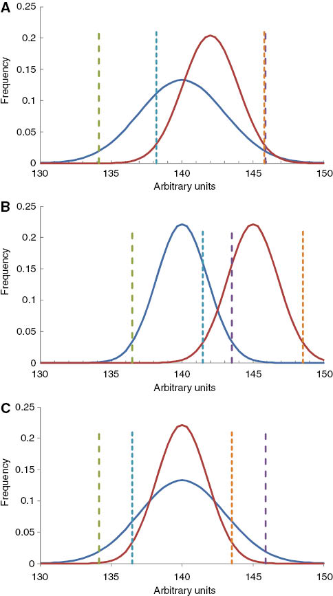
Distribution patterns of two population subsets of which the reference limits are to be compared.
Green broken line: lower RL of distribution (procedure) A, RL1A; blue broken line: lower RL of distribution (procedure) B, RL1B; violet broken line RL2A; red broken line: RL2B. Blue line: distribution A, red line distribution B. The axes are given in arbitrary units.
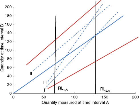
Regression lines between the lower and upper reference limits.
Vertical black lines represent the reference limits of procedure A (abszissa). The scales of the two axes are identical with arbitrary units of the two analytical procedures (A and B) or of measured quantities obtained with the same procedure at different time intervals (A and B). The units differ of those in Figure 1. The red lines are the upper and lower equivalence limit lines. The blue, broken regression lines I (Figure 1A), II (Figure 1B) and III (Figure 1C) correspond to the examples shown in Figure 1.
The equivalence lines are based on the permissible analytical uncertainty of procedure A (pCVA). The multiplication factor for pCVA was chosen arbitrarily as about 1.3 because it appeared to provide plausible permissible limits. This factor happened to correspond to the 90% quantile of the normal distribution (one-sided confidence interval of about 90%). Then, the upper equivalence line in Figure 2 is defined as
and the lower equivalence line is
In these equations, xi represents values from subgroup A, yi represents values from subgroup B, and pu denotes the permissible uncertainty of xi. In the theoretical example of Figure 2, the permissible analytical imprecision at RL1 is lower than at RL2. The equivalence lines are analogous to equivalence limits proposed for method comparison studies [8].
Assuming that RLA and RLB are determined without bias or with the same bias, the permissible uncertainty pu can be reduced to the analytical standard deviation psA (pu=psA). Bias may be considered if RL from external sources are compared with each other and the bias of both analytical procedures is either unknown or presumably different. Then, pu may become 1.22·psA as recently proposed [9].
For simplification, instead of equivalence lines, only both ends of a reference interval (RI) are tested independently. If bias can be neglected, the absolute difference D1(=|RL1A–RL1B|) between the two lower RL (RL1A and RL1B) should not exceed a permissible difference (pD1)
and the absolute difference D2 between the two upper RLs (RL2A and RL2B) should not exceed a permissible difference
Figure 2 shows the permissible differences. pD1 is the distance between the intersection of the vertical RL1 line with the blue diagonal line and the intersection of the RL1 line with the upper or the lower equivalence line. Analogously, pD2 is the distance between the intersection of the vertical RL2 line with the blue diagonal and the intersection of the RL2 line with the upper or lower equivalence line.
In the proposed approach, the length of the measurement series for estimating the analytical variation is assumed to be n=20 and that the effect of larger series lengths can be neglected [10]. According to international recommendations [7, 11], laboratories should know their permissible uncertainties. If this is not the case, psA values can be calculated (equation 10 in the Appendix) from the corresponding pCVA values taken from published sources, e.g. by Ricos [12] or by Haeckel et al. [9]. The latter list may be preferred because permissible limits can be calculated for any quantity of a measurand based on the biological variation. A list with pCVA,Xi values for 84 measurands is available from the home page of the German Society for Clinical Chemistry and Laboratory Medicine [13]. This list is part of an Excel platform for the calculation of permissible uncertainty of any quantitative measurand. The algorithms for calculating pD1 and pD2 (equations 3 and 4) are also included. The interested reader finds a summary of the corresponding algorithms in the Appendix.
Results
Some practical examples of permissible differences (pD%) are listed in Table 1. The examples shown in Table 1 are compared with limits suggested by CSLI [2]. The CLSI recommendation is based on a proposal of Harris and Boyd [3]. It is assumed that s1=s2 and d=mean2–mean1. This approach considers only the distance between mean values, their standard deviations and depends on the number of contributing values (see Appendix). In most cases, the permissible differences were higher than those from our proposal. With sodium, the permissible difference of CLSI (0.70%=1.02 mmol/L at 145 mmol/L) is probably too stringent for most laboratories. Whereas for quantities with a relative large biological variation, e.g. aspartate aminotransferase (AST), triglycerides and thyreotropine (TSH), the pD% of CLSI were much higher than can be achieved by the present technology. At the upper reference limits, the new proposal leads to pD% values of 1.59% for sodium (pD=2.3 mmol/L), 6.7% for triglycerides (pD=0.09 mmol/L) and 7.4% for TSH (pD=0.2 mU/L) which appear plausible under the present technologies.
The relation between permissible differences (pD), percent permissible differences (pD in% of RL1 or RL2) demonstrated with venous blood thrombocytes and some plasma quantities.
| Quantity | Unit | CVE*a | RL1b | RL2 | pD (RL1)c | pD (RL2)c | pD% (RLL)d | pD% (RL2)e | pD%f (CSLI) |
|---|---|---|---|---|---|---|---|---|---|
| Ca ionized | mmol/L | 5.92 | 1.15 | 1.45 | 0.04 | 0.04 | 3.12 | 2.98 | 2.29 |
| Sodium | mmol/L | 1.82 | 135 | 145 | 2.18 | 2.31 | 1.62 | 1.59 | 0.70 |
| Potassium | mmol/L | 6.54 | 3.6 | 4.65 | 0.12 | 0.15 | 3.30 | 3.14 | 2.53 |
| Glucose | mmol/L | 12.69 | 3.9 | 6.4 | 0.19 | 0.28 | 4.76 | 4.31 | 4.91 |
| Creatinine | μmol/L | 18.84 | 50 | 104 | 3.00 | 5.39 | 6.00 | 5.18 | 7.30 |
| AST | U/L | 32.79 | 10 | 35 | 0.86 | 2.32 | 8.58 | 6.62 | 12.70 |
| Triglycerides | mmol/L | 33.49 | 0.39 | 1.40 | 0.03 | 0.09 | 8.70 | 6.68 | 12.97 |
| TSH | mU/L | 42.85 | 0.5 | 2.5 | 0.05 | 0.19 | 10.42 | 7.44 | 16.60 |
| PSA | μg/L | 52.54 | 0.27 | 1.87 | 0.03 | 0.15 | 12.28 | 8.10 | 20.35 |
| Thrombocytes | × 109/L | 14.24 | 210 | 366 | 10.70 | 16.68 | 5.09 | 4.56 | 5.52 |
aEmpirical biological coefficient of variation derived of the logarithmic scale, taken from Ref. [9]. bRL1 lower reference limit, RL2 upper reference limit, taken from Ref. [9], or, for creatinine from Ref. [14]. cCalculated by equations (3) and (4).dpD (RL1)×100/RL1. epD (RL2)×100/RL2. fpD in % of the upper RL according to Harris and Boyd [2, 3]: if s1=s2=sE: D%=3[2(CVE2/n)]0.5; see Appendix.
The applicability of the permissible differences presented in Table 1 is demonstrated by two practical examples: plasma creatinine and AST. An upper RL for creatinine of 104 μmol/L has been found with men and of 88 μmol/L with women [14]. This difference of 16 is above the pD of about 5 μmol/L reported in the table. Therefore, stratification according to gender can be justified. The upper RL of AST for women is 35.0 U/L. If a laboratory finds 37.0 U/L, the difference is not relevant, because the difference of 2.0 U/L is less than the permissible difference of 2.3 U/L.
The calculations behind the results of Table 1 can be performed on the Excel platform. The Excel platform with the algorithms required can be obtained from the authors or from the homepage of the DSRL [13] gratuitously.
Discussion
Differences between two RLs derived of two population subsets can have different components:
biological differences of the distribution pattern (differences in shape, in modes, in variation due to age, gender, race or other genetic causes),
analytical differences. The two RLs may be determined by analytical procedures with different imprecision and/or with different bias.
If analytical reasons for an identified difference can be found (e.g. bias), the reason may be eliminated and the testing repeated afterwards. If analytical reasons can be excluded and biological causes are suspected (different sex or age in a population examined under the same analytical conditions), stratification is recommended. For the purpose of combining RLs (to create common RLs), only analytical variation may be acceptable (within specified limits). All other factors should be either excluded (if detected) or, if suspected, are reasons for stratification. Only if the difference between RLs is higher than can be explained by analytical causes, RLs should be stratified.
Differentiation between analytical and biological causes may not be easy. Therefore in practice, RLs of one subset should not be modified by using additional data from another subset more than would be allowed for analytical reasons only (in the absence of biological reasons). If an inacceptable change occurs, a significant biological reason is assumed, and/or the random error or the bias inherent in one RL is too large to justify combining the two subgroups. Although the relevance of D in equations 3 and 4 is based on pCVA, it may also include small differences in biological variation. pCVA is taken from Ref. [9], as also explained in the Appendix, and is related to the biological variation and preferably to the established RL (procedure A) or to the RL with the lower value.
In equation 1 and 2, a factor of 1.28 was chosen corresponding to the 90% quantile of the normal distribution. This confidence interval could be changed by applying a higher factor, e.g. 1.64. This would increase the confidence interval to e.g. 95% with the disadvantage of higher rates of false negative results. The 90% confidence interval for equivalence limits is analog to the recommendation of IFCC [15] for confidence intervals of reference limits.
Benefits of the present proposal in comparison with other concepts [2, 4, 5]: it
considers biological variation;
is prevalence independent;
does not require approximately equally large sub-populations;
can be used for stratification purposes and for comparing two RLs which are suspected to emerge from the same population. The latter purpose fulfills the requirements for periodic reviewing of RLs as, e.g. postulated by the former ISO standard 15189 [7];
can be applied if only one (lower or upper) RL of the RI is known. However, the indirect model developed by a working group of the German Society for Clinical chemistry and laboratory medicine (DGKL) always yields both ends of a reference interval and can be used [13].
Conclusions
The model proposed can simply be applied by equations (5) and (6), and by taking permissible CVA values from already published lists.
Limitations
As already pointed out by Katayev et al. [16] all models for estimating reference limits, their confidence limits and equivalence limits are based on assumptions which are more or less close to the reality. The IFCC approach is usually considered as the best scientific one, but appears to be most ideal and less realistic than those which are based on a large bulk of a mixed population. Independent on how reference limits are derived, a simple model is required for a fast estimation of permissible differences. Stratification concepts are designed for reference limits, but not for action limits [17].
The approach proposed may be considered as a first approach because it neglects the influence of the number of contributing values. Considering this influence would need much more complex algorithms.
Author contributions: All the authors have accepted responsibility for the entire content of this submitted manuscript and approved submission.
Research funding: None declared.
Employment or leadership: None declared.
Honorarium: None declared.
Competing interests: The funding organization(s) played no role in the study design; in the collection, analysis, and interpretation of data; in the writing of the report; or in the decision to submit the report for publication.
Appendix
Estimation of permissible variation
The permissible analytical variation pCVA and the empirical (biological variation) CVE are derived as recently described [9]. CVE is only considered as a surrogate for the biological variation because it also includes the analytical variance. It is derived from the upper and lower reference limits. In the case of a normal distribution CVE=(RL2–RL1)/3.92. Because the distribution of most quantities is not known, a log-normal distribution may be assumed [18], and CVE becomes CVE*.
Assuming log-normally distributed data, standard deviation and median on the logarithmic scale sE,ln and Medln can be calculated by the following equation
On the logarithmic scale, mean and median are identical. The arithmetic mean and standard deviation on the linear scale are according to Ref. [19–21]:
From these, CVE* valid on the linear scale can be calculated by equations 7 and 8
The permissible CVA at the median on the linear scale [Med=exp(Medln)=(RL1·RL2)0.5] can be obtained from CVE* by equation 9 as explained in Ref.[9]:
From this, the permissible analytical standard deviation at the median is
The analytical standard deviation is assumed to increase linearly with the measured value xi and can be calculated at any xi by equations 11 and 12:
The slope a in equation 11 is
and the intercept b is
The permissible standard deviation at xi is
This can be expressed as coefficient of variation:
The intercept b in equation 11 is related to the detection limit. Because the detection limit is usually unknown for the matrix of human materials, 20% of the sA at the median is applied here as a substitute.
Comparison of several reference limits
In the case of comparing several RLs (RLiA, RLiB, RLiC, …, i=1,2), the difference between the highest and lowest RL is compared with psA as described above (equations 5 and 6). If the difference exceeds 1.28·psA, one RL is excluded, and the maximal difference between the remaining RLs is tested again.
Harris and Boyd approach
The Harris and Boyd approach is based on the standard normal deviate test [2, 3]:
References
1. Haeckel R, Wosniok W, Arzideh F. A plea for intra-laboratory reference limits Part 1. General considerations and concepts for determination. Clin Chem Lab Med 2007;45:1033–42.10.1515/CCLM.2007.249Search in Google Scholar
2. CLSI/IFCC. Defining, establishing, and verifying reference intervals in the clinical laboratory; approved guideline – third edition. CLSI document C28-P3. Wayne, PA: Clinical and Laboratory Standards Institute, 2008;28:1–50.Search in Google Scholar
3. Harris EK, Boyd JC. On dividing reference data into subgroups to produce separate reference ranges. Clin Chem 1990;36:265–70.10.1093/clinchem/36.2.265Search in Google Scholar
4. Lahti A, Hylthoft Petersen R, Boyd JC. Impact of subgroup prevalences on partitioning of Gaussian-distributed reference values. Clin Chem 2002;48:1987–99.10.1093/clinchem/48.11.1987Search in Google Scholar
5. Lahti A, Hylthoft Petersen R, Boyd JC, Rustad P, Laake P, Solberg HE. Partitioning of nongaussian-distributed biochemical reference data into subgroups. Clin Chem 2004;50:891–900.10.1373/clinchem.2003.027953Search in Google Scholar
6. Gellerstedt M, Hylthoft Petersen P. Partitioning reference values for several subpopulations using cluster analysis. Clin Chem Lab Med 2007;45:1026–32.10.1515/CCLM.2007.192Search in Google Scholar
7. International Standard Organisation. Medical Laboratories – particular requirements for quality and competence, ISO 15189, 2nd ed, 2007:1–40 (Note that a third edition is in preparation).Search in Google Scholar
8. Haeckel R, Wosniok W, Al Sahreef N. Permissible performance limits of regression analyses in method comparisons. Clin Chem Lab Med 2011;49:1805–16.10.1515/cclm.2011.668Search in Google Scholar
9. Haeckel R, Wosniok W, Gurr E, Peil B. Permissible limits for uncertainty of measurement in laboratory medicine. Clin Chem Lab Med 2015;53:1161–71.10.1515/cclm-2014-0874Search in Google Scholar
10. Haeckel R, Wosniok W, Gurr E, Wosniok W, Peil B. Supplements to a recent proposal for permissible uncertainty of measurements in laboratory medicine. J Lab Med 2016;40:141–5.10.1515/labmed-2015-0112Search in Google Scholar
11. International Standard Organisation. In vitro diagnostic test systems – requirements for blood glucose monitoring systems for self-testing in managing diabetes mellitus. ISO 15197, 1st ed. 2003:1–33.Search in Google Scholar
12. Ricos C, Garcia-Lario JV, Alvarez V, Cava F, Domenech M, Hemander A, et al. 2008. www.westgard.com/guest17.htm, updated 2008.Search in Google Scholar
13. Permissible imprecision (pCVA) and combined uncertainty (pU%) for a particular measurand (xi). www.dgkl.de, assessed 01.03.2015.Search in Google Scholar
14. Arzideh F, Wosniok W, Haeckel R. Reference limits of plasma and serum creatinine concentrations from intra-laboratory data bases of several German and Italian medical centres. Comparison between direct and indirect procedures. Clin Chim Acta 2010;411:215–21.10.1016/j.cca.2009.11.006Search in Google Scholar
15. Solberg HE. Approved recommendation (1987) on the theory of reference values. Part 5: Statistical treatment of collected reference values. Determination of reference limits. J Clin Chem Clin Biochem 1987;25:645–56.10.1016/0009-8981(87)90151-3Search in Google Scholar
16. Katayev A, Balciza C, Seccombe DW. Establishing reference intervals for clinical laboratory test results. Is there a better way? Am J Clin Pathol 2010;133:180–6.10.1309/AJCPN5BMTSF1CDYPSearch in Google Scholar PubMed
17. Haeckel R, Wosniok W, Arzideh F. Proposed classification of various limit values (guide values) used in assisting the interpretation of quantitative laboratory test results. Clin Chem Lab Med 2009;47:494–7.10.1515/CCLM.2009.043Search in Google Scholar PubMed
18. Haeckel R, Wosniok W. Observed unknown distributions of clinical chemistry quantities should be considered to be log-normal: a proposal. Clin Chem Lab Med 2010;48: 1393–6.10.1515/CCLM.2010.273Search in Google Scholar PubMed
19. Aitchison J, Brown JA. The lognormal distribution. Cambridge: University Press, 1969:1–176.Search in Google Scholar
20. Johnson NL, Katz S, Balakrishnan N. Continuous univariate distributions. New York: J. Wiley & Sons, Inc., 1994:1–756.Search in Google Scholar
21. https://en.wikipedia.org/wiki/log-normal_distribution.Search in Google Scholar
©2016 by De Gruyter
This article is distributed under the terms of the Creative Commons Attribution Non-Commercial License, which permits unrestricted non-commercial use, distribution, and reproduction in any medium, provided the original work is properly cited.
Articles in the same Issue
- Frontmatter
- Labormanagement/Laboratory Management / Redaktion: E. Wieland
- Der Einfluss der DIN EN ISO 15189 auf die Ergebnissicherheit in der Virusdiagnostik
- Entzündung und Sepsis/Inflammation and Sepsis / Redaktion: P. Fraunberger
- HMGB1, nucleosomes and sRAGE as new prognostic serum markers after multiple trauma
- Infektiologie und Mikrobiologie (Schwerpunkt Bakteriologie)/Infectiology and Microbiology (Focus Bacteriology) / Redaktion: P. Ahmad-Nejad/B. Ghebremedhin
- Improvement in detecting bacterial infection in lower respiratory tract infections using the Intensive Care Infection Score (ICIS)
- Evaluation of the compatibility of Phoenix 100 and Microflex LT MALDI-TOF MS systems in the identification of routinely isolated microorganisms in the clinic microbiology laboratory
- Mini Review
- Liquorzytologie: Eine aussagekräftige Methode zur Diagnostik von Erkrankungen des Zentralnervensystems
- Opinion Paper
- Equivalence limits of reference intervals for partitioning of population data. Relevant differences of reference limits
- Originalartikel/Original Articles
- Influence of uvulopalatopharyngoplasty on serum uric acid level in obstructive sleep apnea patients
- Correlation between severity of migraine attacks and IgE level in peripheral blood
- Kurzmitteilung/Short Communication
- Comparison of the novel Maglumi ferritin immunoluminometric assay with Beckman Coulter DxI 800 ferritin