Temporally Local Maximum Likelihood with Application to SIS Model
-
Christian Gourieroux


Abstract
The parametric estimators applied by rolling are commonly used for the analysis of time series with nonlinear patterns, including time varying parameters and local trends. This paper examines the properties of rolling estimators in the class of temporally local maximum likelihood (TLML) estimators. We consider the TLML estimators of (a) constant parameters, (b) stochastic, stationary parameters and (c) parameters with the ultra-long run (ULR) dynamics bridging the gap between the constant and stochastic parameters. We show that the weights used in the TLML estimators have a strong impact on the inference. For illustration, we provide a simulation study of the epidemiological susceptible–infected–susceptible (SIS) model, which explores the finite sample performance of TLML estimators of a time varying contagion parameter.
Funding source: Natural Sciences and Engineering Research Council of Canada
-
Research funding: The first author acknowledges financial support from the ACPR chair “Regulation and Systemic Risk”, the ERC DYSMOIA and the Agence Nationale de la Recherche (ANR-COVID) [Grant ANR-17-EURE-0010]. The second author gratefully acknowledges financial support of the Natural Sciences and Engineering Council of Canada (NSERC).
-
Conflict of interest statement: The authors declare no conflicts of interest regarding this article.
-
Author contribution: All the authors have accepted responsibility for the entire content of this submitted manuscript and approved submission.
Appendix A: Second-Order Expansion
Even though the TLML estimator is consistent, the finite sample bias adjustment formula is expected to be non-standard. We consider below the second-order expansion of the FOC [see Gosh and Subramanyan (1974), Efron (1975), Firth (1993), Kosmidis and Firth (2009)]. For expository purpose, we assume dim θ t = 1. We define:
The second-order expansion of the FOC in a neighbourhood of the pseudo-true value is:
where o p is negligible in probability with respect to the left hand side of the equation, or equivalently,
From (3.9), it follows that:
where X T ∼ N(0, 1).
This expression can be plugged into the two last terms of the second-order expansion to get:
Let us consider the variable:
where
Then we get:
This expansion provides an approximation of the difference between the TLML estimator and the pseudo-true value as a quadratic function of the pair (X T , Z T ), which is asymptotically normally distributed and has zero mean components with unitary variances and non-zero correlation, in general. Alternative bias adjustments could be based on the pseudo score [Lambrecht et al. (1997)].
Appendix B: Stationarity Condition
B.1 Condition for Ergodicity
Whenever the Markov chain is irreducible, we can use the sufficient conditions for ergodicity provided in Tweedie (1975). They are:
Let us now consider condition (ii). We have:
Therefore condition (ii) is satisfied with the compact set K = [ɛ/c, 1], and ɛ < c.
B.2 Condition for Irreducibility
The different types of behaviour discussed below Proposition 6 are related to the irreducibility properties of the Markov chain [see e.g. Rio (2017), Chapter 9, and Chotard and Auger (2019)]. This irreducibility follows from the condition 0 < 1 − c/a < 1, and replacing of
Appendix C: Additional Figures
C.1 Quasi-Collinearity
To provide some insights on the quasi-collinearity, we compute the sample information matrix from the Hessian of the temporally local log-likelihood function and report its eigenvalues. As expected these eigenvalues are positive and one of them is small and close to 0.
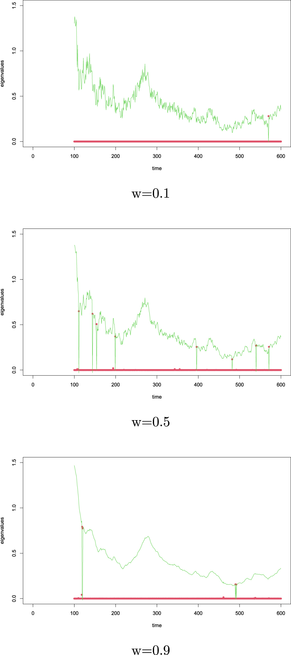
Eigenvalues of estimated information matrix: Constant a.
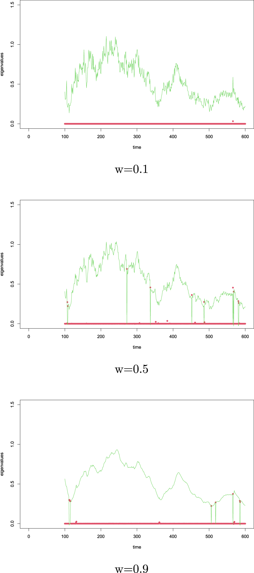
Eigenvalues of estimated information matrix: Stochastic a.
C.2 Persistence of Estimates and Stochastic Parameters
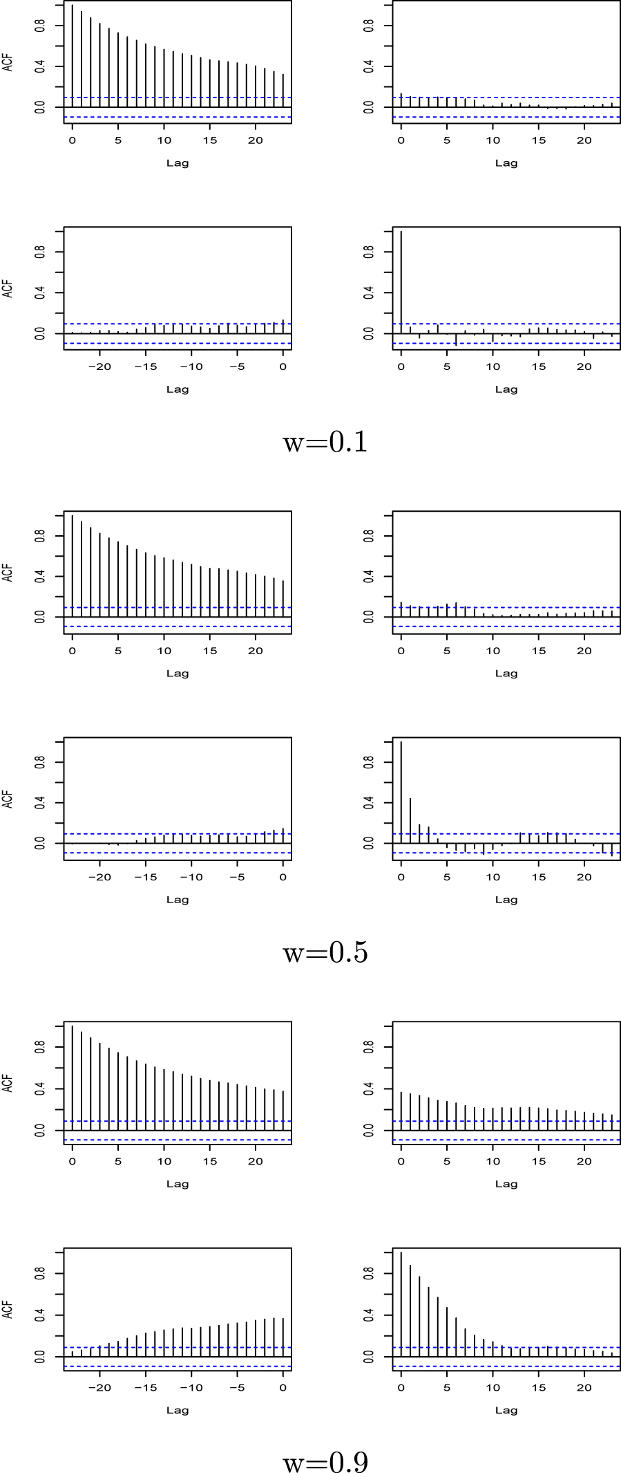
Additional summary statistics provided below concern the joint dynamics of the stochastic parameters of interest and their local estimates. They are displayed in Figures 14 and 15 for the contagion parameter and reproductive number, respectively. For each value of w considered, the diagonal panels show the autocorrelations of the estimates and of the stochastic parameters, respectively. The off-diagonal panels show the cross-correlations between the estimates and stochastic parameters.
Joint ACF of a
t
and
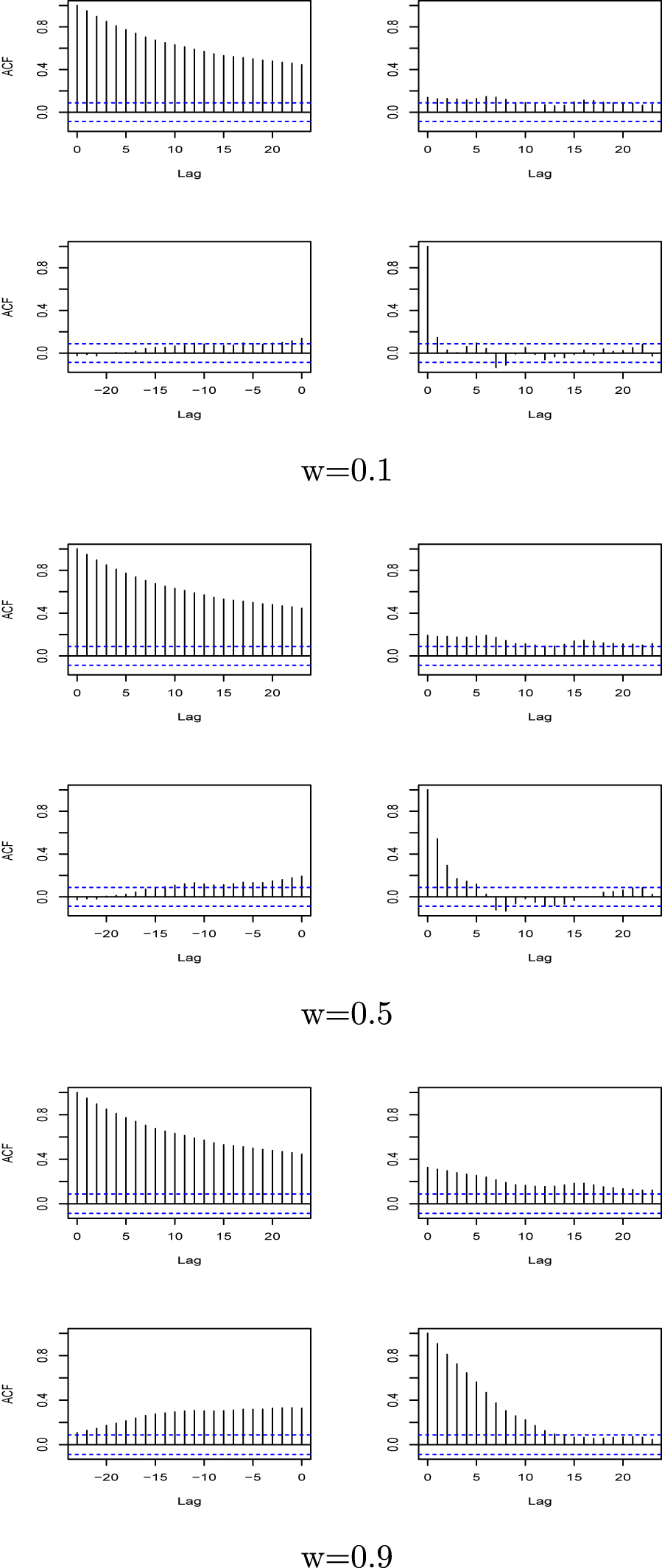
Joint ACF of R0,t and
The autocorrelation function (ACF) of a
t
and R0,t reveals the local-to-unity property of the ULR process. For w = 0.1, the weighted estimator is more global and appears almost uncorrelated with the underlying stochastic parameter. We observe that the cross-correlations, which often take small values, do not decay to zero with the lag. This is a consequence of the ULR a
t
process. For larger w, the estimates display more persistence, although the autocorrelations of
C.3 Nonlinear Prediction Performance
Under the standard maximum likelihood approach, the values of the log-likelihood at the optimum can be used to perform tests based on the likelihood ratios, especially of the time varying hypotheses H0T = {R0T > 1}. It can be used to check the “joint” accuracy of
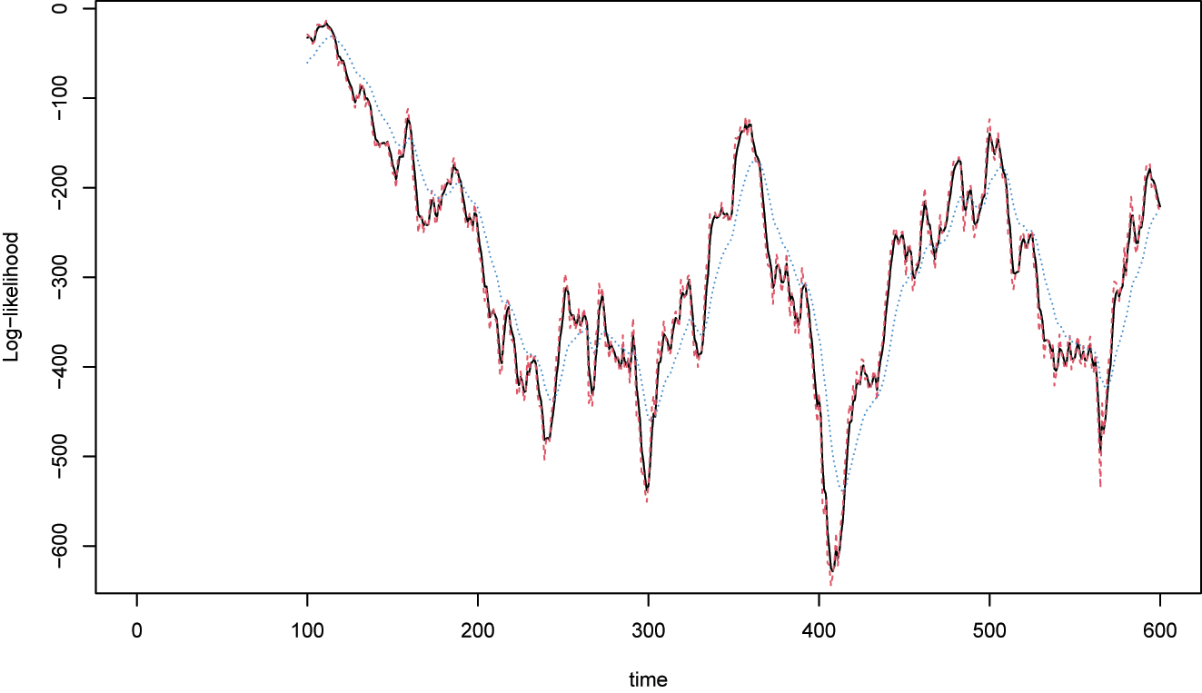
Log-likelihoods, stochastic a, red dashed line: w = 0.1, black solid line: w = 0.5 and dotted green line: w = 0.9.
This evolution has to be compared with the trajectory of counts in Figure 6. As expected, the local nonlinear fit is improved during the episodes of counts evolving without sudden jumps or “local” trends, i.e. characterized by rather stable evolution. In contrast, the values of the log-likelihood are shown to decrease in the neighbourhoods of peaks or troughs.
Alternative measures of prediction performance could also be built by comparing at each date the observed number of infected individuals N2(t) with its estimator-based prediction:
The difference
References
Anderes, E., and M. Stein. 2011. “Local Likelihood Estimation for Nonstationary Random Fields.” Journal of Multivariate Analysis 102: 506–20. https://doi.org/10.1016/j.jmva.2010.10.010.Suche in Google Scholar
Andrews, D. 1987. “Consistency in Nonlinear Econometric Models; A Generic Uniform Law of Large Numbers.” Econometrica 55: 1465–71. https://doi.org/10.2307/1913568.Suche in Google Scholar
Brauer, F., L. Allen, P. Van den Driessche, and J. Wu. 2008. Mathematical Epidemiology In Lecture Notes in Mathematics, 1945, Mathematical Biosciences Subseries. Berlin Heidelberg: Springer.10.1007/978-3-540-78911-6Suche in Google Scholar
Breto, C., D. He, E. Ionides, and A. King. 2009. “Time Series Analysis via Mechanistic Models.” Annals of Applied Statistics 3: 319–48. https://doi.org/10.1214/08-aoas201.Suche in Google Scholar
Cai, Z. 2007. “Trending Time-Varying Coefficient Time Series Models with Serially Correlated Errors.” Journal of Econometrics 136: 163–88. https://doi.org/10.1016/j.jeconom.2005.08.004.Suche in Google Scholar
Cai, Z., J. Fan, and R. Li. 2000. “Efficient Estimation and Inferences for Varying-Coefficient Models.” Journal of the American Statistical Association 95: 838–902. https://doi.org/10.1080/01621459.2000.10474280.Suche in Google Scholar
Calafiore, G., C. Novara, and C. Possieri. 2020. “A Modified SIR Model for the COVID-19 Contagion in Italy.” ArXiv 2003.14301.10.1109/CDC42340.2020.9304142Suche in Google Scholar
Canova, F., and J. P. Forero. 2015. “Estimating Overidentified Nonrecursive Time-Varying Coefficients Structural Vector Autoregressions.” Quantitative Economics 6: 359–84. https://doi.org/10.3982/qe305.Suche in Google Scholar
Carpenter, J. 1999. “Test Inversion Bootstrap Confidence Intervals.” Journal of the Royal Statistical Society - Series B 61: 159–72. https://doi.org/10.1111/1467-9868.00169.Suche in Google Scholar
Chotard, A., and A. Auger. 2019. “Verifiable Conditions for the Irreducibility and Aperiodicity of Markov Chains by Analyzing Underlying Deterministic Models.” Bernoulli 25: 112–47. https://doi.org/10.3150/17-bej970.Suche in Google Scholar
Cooke, K., and J. Yorke. 1973. “Some Equations Modelling Growth Processes and Gonorrhea Epidemics.” Mathematical Biosciences 16: 75–101. https://doi.org/10.1016/0025-5564(73)90046-1.Suche in Google Scholar
Cori, A., N. Ferguson, C. Fraser, and S. Cauchemez. 2013. “A New Framework and Software to Estimate Time Varying Reproduction Numbers during Epidemics.” American Journal of Epidemiology 178: 1505–12. https://doi.org/10.1093/aje/kwt133.Suche in Google Scholar PubMed PubMed Central
Dahlhaus, R. 2012. “Locally Stationary Processes.” In Handbook of Statistics, 30, 351–412. North Holland, Amsterdam: North Holland Publishing Company.10.1016/B978-0-444-53858-1.00013-2Suche in Google Scholar
Dahlhaus, R., S. Richter, and W. Wu. 2019. “Towards a General Theory of Nonlinear Locally Stationary Processes.” Bernoulli 25: 1013–44.10.3150/17-BEJ1011Suche in Google Scholar
Das, P., D. Mukherjee, and A. Sarkar. 2011. “Study of an SI Epidemic Model with Nonlinear Incidence Rate: Discrete and Stochastic Version.” Applied Mathematics and Computation 218: 2509–15. https://doi.org/10.1016/j.amc.2011.07.065.Suche in Google Scholar
Dureau, J., K. Kalogeropoulos, and M. Buguelin. 2013. “Capturing the Time Drivers of an Epidemic Using Stochastic Dynamical Systems.” Biostatistics 14: 541–55. https://doi.org/10.1093/biostatistics/kxs052.Suche in Google Scholar PubMed
Efron, B. 1975. “Defining the Curvature of a Statistical Problem (With Applications to Second-Order Efficiency).” Annals of Statistics 3: 1189–242. https://doi.org/10.1214/aos/1176343282.Suche in Google Scholar
Elliot, S., and C. Gourieroux. 2021. “Estimated Reproduction Ratios in the SIR Model.” Canadian Journal of Statistics 49: 992–1017. https://doi.org/10.1002/cjs.11663.Suche in Google Scholar PubMed PubMed Central
Fan, J., and I. Gijbels. 1996. Local Polynomial Modelling and its Applications. New York: Chapman and Hill.Suche in Google Scholar
Fan, J., and W. Zhang. 2000. “Simultaneous Confidence Bands and Hypothesis Testing in Varying Coefficient Models.” Scandinavian Journal of Statistics 27: 715–31. https://doi.org/10.1111/1467-9469.00218.Suche in Google Scholar
Fahrmeir, L., and H. Kauffmann. 1985. “Consistency and Asymptotic Normality of the Maximum Likelihood Estimator in the Generalized Linear Models.” Annals of Statistics 13: 342–68.10.1214/aos/1176346597Suche in Google Scholar
Firth, D. 1993. “Bias Reduction of Maximum Likelihood Estimates.” Biometrika 80: 27–38. https://doi.org/10.1093/biomet/80.1.27.Suche in Google Scholar
Francq, C., and A. Gautier. 2004. “Estimation of Time Varying ARMA Models with Markovian Changes in Regimes.” Statistics & Probability Letters 70: 243–51. https://doi.org/10.1016/j.spl.2004.10.009.Suche in Google Scholar
Froeb, L., and R. Koyak. 1994. “Measuring and Comparing Smoothness in Time Series: The Production Smoothing Hypothesis.” Journal of Econometrics 64: 97–122. https://doi.org/10.1016/0304-4076(94)90059-0.Suche in Google Scholar
Godambe, V., and C. Heyde. 1987. “Quasi-Likelihood and Optimal Estimation.” International Statistical Review 55: 231–44.10.2307/1403403Suche in Google Scholar
Gosh, J., and K. Subramanyan. 1974. “Second-Order Efficiency of Maximum Likelihood Estimators.” Sankhya, A. 36: 325–58.Suche in Google Scholar
Gourieroux, C., and J. Jasiak. 2020. “Analysis of Virus Transmission: A Transition Model Representation of Stochastic Epidemiological Models.” Annals of Economics and Statistics 140: 1–26. https://doi.org/10.15609/annaeconstat2009.140.0001.Suche in Google Scholar
Gourieroux, C., and J. Jasiak. 2022a. “Long Run Risk in Stationary Structural Vector Autoregressive Models.” ArXiv 2202.09473.Suche in Google Scholar
Gourieroux, C., and J. Jasiak. 2022b. “Long Run Predictions.” Annals of Economics and Statistics 145: 75–90. https://doi.org/10.2307/48655902.Suche in Google Scholar
Gourieroux, C., J. Kim, and N. Meddahi. 2022. Stationary Ultra Long Run Component. CREST DP.Suche in Google Scholar
Gourieroux, C., and Y. Lu. 2020. SIR Model wtih Stochastic Transmission. CREST DP.10.2139/ssrn.3730349Suche in Google Scholar
Gray, A., D. Greenhalgh, L. Hu, X. Mao, and J. Pan. 2011. “A Stochastic Differential Equation SIS Epidemic Model.” SIAM Journal on Applied Mathematics 71: 876–902. https://doi.org/10.1137/10081856x.Suche in Google Scholar
Greenberg, J., and F. Hoppensteadt. 1975. “Asymptotic Behaviour of Solutions to a Population Equation.” SIAM Journal on Applied Mathematics 28: 662–74. https://doi.org/10.1137/0128055.Suche in Google Scholar
Hansen, B. 1992. “Convergence to Stochastic Integrals for Dependent Heterogeneous Processes.” Econometric Theory 8: 489–500. https://doi.org/10.1017/s0266466600013189.Suche in Google Scholar
Hastie, T., and R. Tibshirani. 1993. “Varying Coefficient Models.” Journal of the Royal Statistical Society: Series B 55: 757–96. https://doi.org/10.1111/j.2517-6161.1993.tb01939.x.Suche in Google Scholar
Hethcote, H., and P. Van den Driessche. 1995. “An SIS Epidemic Model with Variable Population Size and a Delay.” Journal of Mathematical Biology 34: 177–94. https://doi.org/10.1007/bf00178772.Suche in Google Scholar
Hethcote, H., and J. Yorke. 1994. Gonorrhea Transmission Dynamics and Control In Lecture Notes in Biomathematics, vol. 56. Berlin: Springer-Verlag.Suche in Google Scholar
Ho, P., T. Lubik, and C. Matthes. 2023. “How to Go Viral: A COVID-19 Model with Endogenously Time Varying Parameters.” Journal of Econometrics 232: 70–86. https://doi.org/10.1016/j.jeconom.2021.01.001.Suche in Google Scholar PubMed PubMed Central
Huber, P. 1967. “The Behaviour of Maximum Likelihood Estimates under Nonstandard Conditions.” In Proceedings of the Fifth Berkeley Symposium on Mathematical Statistics and Probability, Vol. 1, 221–33.Suche in Google Scholar
Jennrich, R. 1969. “Asymptotic Properties of Nonlinear Least Squares Estimators.” The Annals of Mathematical Statistics 40: 633–43. https://doi.org/10.1214/aoms/1177697731.Suche in Google Scholar
Kim, C., and C. Nelson. 1999. State Space Models with Regime Switching. Cambridge, MA: Cambridge MIT Press.10.7551/mitpress/6444.001.0001Suche in Google Scholar
Kosmidis, I., and D. Firth. 2009. “Bias Reduction in Exponential Family Nonlinear Models.” Biometrika 96: 793–804. https://doi.org/10.1093/biomet/asp055.Suche in Google Scholar
Lambrecht, B., W. Perraudin, and S. Satchell. 1997. “Approximating the Finite Sample Bias for Maximum Likelihood Estimators Using the Score.” Econometric Theory 13: 310–2. https://doi.org/10.1017/s0266466600005806.Suche in Google Scholar
Lin, D., and Z. Ying. 2001. “Semiparametric and Nonparametric Regression Analysis of Longitudinal Data (With Discussion).” Journal of the American Statistical Association 96: 103–26. https://doi.org/10.1198/016214501750333018.Suche in Google Scholar
Matis, J., and T. Kiffe. 2000. Stochastic Population Models: A Compartmental Perspective. New-York: Springer.10.1007/978-1-4612-1244-7Suche in Google Scholar
McCullagh, P., and J. Nelder. 1989. Generalized Linear Models, 2nd ed. Chapman & Hall.10.1007/978-1-4899-3242-6Suche in Google Scholar
Nicholls, D., and B. Quinn. 1980. “The Estimation of Random Coefficient Autoregressive Model I.” Journal of Time Series Analysis 1: 37–46. https://doi.org/10.1111/j.1467-9892.1980.tb00299.x.Suche in Google Scholar
Primiceri, G. 2005. “Time Varying Structural Vector Autoregressions and Monetary Policy.” The Review of Economic Studies 72: 821–52. https://doi.org/10.1111/j.1467-937x.2005.00353.x.Suche in Google Scholar
Public Health Ontario (PHO). 2021. Enhanced Epidemiological Summary: Trends of COVID-19 Incidence in Ontario. 2021-05-23.Suche in Google Scholar
Rifhat, A., L. Wang, and Z. Teng. 2017. “Dynamics for a Class of Stochastic SIS Epidemic Models with Nonlinear Incidence and Periodic Coefficients.” Physica A 480: 176–90. https://doi.org/10.1016/j.physa.2017.04.016.Suche in Google Scholar
Rio, E. 2017. Asymptotic Theory of Weakly Dependent Random Processes In Probability Theory and Stochastic Modelling, vol. 80. Berlin Heidelberg: Springer.10.1007/978-3-662-54323-8Suche in Google Scholar
Rubio-Herrero, J., and Y. Wang. 2021. “A Flexible Rolling Regression Framework for Time-Varying SIRD Model: Application to COVID-19.” ArXiv 2103.02048.Suche in Google Scholar
Shapiro, M., F. Karim, G. Murcioni, and A. Augustine. 2020. Are We There Yet? An Adaptive SIR Model for Continuous Estimation of COViD-19 Infections Rate and Reproduction Number in the United States. DP Anthem, Inc.10.1101/2020.09.13.20193896Suche in Google Scholar
Stroock, D., and S. Varadhan. 1979. Multidimensional Diffusion Processes. Berlin Heidelberg: Springer.Suche in Google Scholar
Tweedie, R. 1975. “Sufficient Conditions for Ergodicity and Recurrence of Markov Chains on a General State Space.” Stochastic Processes and their Applications 3: 385–403. https://doi.org/10.1016/0304-4149(75)90033-2.Suche in Google Scholar
Varin, C., N. Reid, and D. Firth. 2011. “An Overview of Composite Likelihood Methods.” Statistica Sinica 21: 5–42.Suche in Google Scholar
Waqas, M., M. Farooq, R. Ahmed and A. Ahmed. 2020. “Analysis and Prediction of COVID-19 Pandemic in Pakistan Using Time Dependent SIR Model.” ArXiv: 2005.02353.Suche in Google Scholar
Wallinga, J., and P. Teunis. 2004. “Different Epidemic Curves for Severe Acute Respiratory Syndrome Reveal Similar Impacts of Control Measures.” American Journal of Epidemiology 160: 509–16. https://doi.org/10.1093/aje/kwh255.Suche in Google Scholar PubMed PubMed Central
White, H. 1982. “Maximum Likelihood Estimation of Misspecified Models.” Econometrica 50: 1–25. https://doi.org/10.2307/1912526.Suche in Google Scholar
Xu, C., and X. Li. 2018. “The Threshold of a Stochastic Delayed SIRS Epidemic Model with Temporary Immunity and Vaccination.” Chaos, Solitons & Fractals 111: 227–34. https://doi.org/10.1016/j.chaos.2017.12.027.Suche in Google Scholar
Yu, Z., L. Liu, D. Bravata, L. Williams, and R. Tepper. 2013. “A Semi-parametric Recurrent Event Model with Time-Varying Coefficients.” Statistics in Medicine 32: 1016–26. https://doi.org/10.1002/sim.5575.Suche in Google Scholar PubMed PubMed Central
Zhou, Z., and W. Wu. 2010. “Simultaneous Inference of Linear Models with Time Varying Coefficients.” Journal of the Royal Statistical Society - Series B 72: 513–31. https://doi.org/10.1111/j.1467-9868.2010.00743.x.Suche in Google Scholar
© 2023 Walter de Gruyter GmbH, Berlin/Boston