Modern and post-modern portfolio theory as applied to moneyline betting

2.1 Actual and expected net proceeds from a moneyline bet

For any particular basketball or football game (for which moneyline betting is available), a moneyline bet can be placed on the home team or alternatively on the visiting team. Let hml represent the moneyline pertaining to a moneyline bet on the home team and vml that pertaining to a moneyline bet on the visiting team. Further, let hrtn represent the winnings per dollar wagered from a successful moneyline bet on the home team and vrtn the analogous quantity for a successful moneyline bet on the visiting team, and observe that

Note that the net proceeds (per dollar wagered) from a moneyline bet, say hnet in the case of a moneyline bet on the home team and vnet in the case of a moneyline bet on the visiting team, is determined by hrtn or vrtn together with the outcome of the game as reflected in the value of the variable dif (which equals the final score of the home team minus the final score of the visiting team). Specifically,

Let us regard dif as a random variable, in which case the events defined by the inequalities dif > 0 and dif < 0 and by the equality dif = 0 are random events. Further, let p = Pr(dif > 0) (i.e., the probability of the game being won by the home team) and q = Pr(dif < 0) (i.e., the probability of the game being won by the visiting team). For the sake of simplicity, let us assume that Pr(dif = 0) = 0, as would be the case in basketball or college football;  or, alternatively, redefine p as p = Pr(dif > 0|dif ≠ 0) and q as q = Pr(dif < 0|dif ≠ 0) (and recall that the event dif = 0 results in a “push”). Then,

and the expected value of the net proceeds from a moneyline bet is

depending on whether the bet is on the home team or on the visiting team.

The moneylines hml and vml are established by the so-called sportsbook. One way to approach the establishment of hml and vml is to specify a value for p or for p/q (the odds of the game being won by the home team) and to require that

where α is a small positive constant to be specified;  α is interpretable as the fraction of the money expected to be taken in from the losing bettors that is expected to be diverted from distribution to the winning bettors and retained by the betting proprietor, and it reflects what is commonly known as the “vig” (as in vigorish) or the “juice”. Condition (2) is reexpressible in the form

where vrat = (vrtn + 1)/tot and tot = hrtn + vrtn + 2. Moreover, condition (3) is satisfied (uniquely) by taking

or equivalently by taking

and ultimately by taking the moneylines hml and vml to be those for which the corresponding hrtn and the corresponding vrtn satisfy condition (4). Clearly, the moneylines generated by this approach could vary greatly depending on how p or p/q is specified.

An alternative way of establishing hml and vml is to adopt an “empirical” approach that makes use of the relative amounts bet on the two opposing teams. Let hdol represent the total amount bet (by all bettors) on the home team and vdol the total amount bet on the visiting team, and observe that if hrtn and vrtn (and hence hml and vml) satisfy the condition formed by the two equalities

then (regardless of which team wins the game) a fraction α of the total amount wagered on the two teams is retained by the betting proprietor. Observe also that condition (5) is equivalent to the condition

where p ̃ = hdol / ( hdol + vdol ) and q ̃ = vdol / ( hdol + vdol ) = 1 − p ̃ . Moreover, condition (6) is analogous to condition (2);   p ̃ and q ̃ in condition (6) correspond to p and q in condition (2). Thus, as is evident from what is essentially the same argument that led to result (4), condition (6) is reexpressible in the form

or in the form

The betting proprietor has no direct control over p ̃ and q ̃ ;  those quantities are determined by the betting public. However, p ̃ and q ̃ can be affected indirectly through the specification of the moneylines. Based on various factors and on past results from seemingly similar situations, it may be possible to approximate hdol as a (strictly increasing) function, say hdol(hrtn), of hrtn and vdol as a (strictly increasing) function, say vdol(vrtn), of vrtn. The determination of hrtn and vrtn (and ultimately of hml and vml) could then be based on the version of condition (5) that results when hdol is taken to be the function hdol(hrtn) and vdol the function vdol(vrtn).

The implementation of such an approach is facilitated by observing that (since p ̃ + q ̃ = 1 ) condition (8) [which is equivalent to condition (5)] is reexpressible in the form

It can be shown that there exists a strictly decreasing function, say h ̃ ( vrtn ) , of vrtn such that hrtn and vrtn satisfy the first of the two equalities that form condition (9) if and only if 0 < vrtn < (1 − 2α)/α and hrtn = h ̃ ( vrtn ) ;  as vrtn increases from 0 to (1 − 2α)/α,   h ̃ ( vrtn ) decreases from (1 − 2α)/α to 0. Moreover, vdol ( vrtn ) / hdol [ h ̃ ( vrtn ) ] is a strictly increasing function of vrtn, and as vrtn increases from 0 to (1 − 2α)/α,   [ h ̃ ( vrtn ) + 1 ] / ( vrtn + 1 ) decreases from (1 − α)/α to α/(1 − α). It follows that unless vdol ( vrtn ) / hdol [ h ̃ ( vrtn ) ] ≤ α / ( 1 − α ) when vrtn = (1 − 2α)/α, the version of condition (5) in which hdol and vdol are taken to be the functions hdol(hrtn) and vdol(vrtn) can be satisfied by taking vrtn to be such that vdol ( vrtn ) / hdol [ h ̃ ( vrtn ) ] = [ h ̃ ( vrtn ) + 1 ] / ( vrtn + 1 ) and setting hrtn = h ̃ ( vrtn ) .

In practice, the moneylines appear to be established via a somewhat convoluted and competitive process undertaken by multiple sportsbooks;  the operative moneylines may be changed from time to time in response to “imbalances” in the betting pattern or to other issues. The moneylines affect the profits of the betting proprietor not only through their effect on the profit margin but also through their effect on the volume of betting. There is a tradeoff;  increasing hrtn and vrtn increases the volume at the expense of smaller margins. To the extent that the moneylines are determined by imposing condition (2) or (5), it is the choice of α that determines where the balance is struck between volume and margin. Some data-driven insights into the operations of the sportsbooks are provided by Levitt (2004).

Had the moneylines been established by imposing condition (2), the underlying p and α would have been as follows:

Alternatively (and similarly), had they been established by imposing condition (5) or equivalently condition (6), the underlying p ̃ and α would have been

In light of results (10) and (11), it could be of interest to consider the quantity p defined (in terms of hrtn and vrtn and ultimately in terms of hml and vml) by the expression

If the moneylines had been determined by the sportsbook based on the imposition of condition (2), then this quantity would represent the probablity they had used in doing so. Alternatively, if the moneylines had been determined based on the imposition of condition (5), then this quantity could be regarded as a probability that had been determined by the bettors themselves;  a probability determined in such a manner is said to have been determined by the “wisdom of the crowd”. In regard to the underlying α, it is informative [in contemplating results (10) and (11)] to consider the case of two “evenly matched” teams (where p or p ̃ equals 0.5). Assuming that hml(=vml) = −110 (as is rather typical in this case),

Now, suppose that the operative p and q are those adopted by a would-be bettor, and observe that from the perspective of a would-be bettor, the moneylines hml and vml are a given. Accordingly, what could be of some interest are the two “breakeven” points, say pmin and qmin, consisting respectively of the smallest value of p for which hmu ≥ 0 and the smallest value of q for which vmu ≥ 0. From result (1), it is evident that

Moreover, if the moneylines were those established by imposing condition (2) or condition (6), then it would be the case that

as can be readily verified. More generally, regardless of how the sportsbook may have arrived at the moneylines, it is invariably the case that

—if pmin + qmin were less than 1, there would exist fractions p* and q* such that p* > pmin, q* > qmin, and p* + q* = 1, and a bettor could achieve a profit regardless of the outcome of the game by betting a fractional amount p* on the home team and a fractional amount q* on the visiting team.

It is also the case that the probabilities pmin/(pmin + qmin) and qmin/(pmin + qmin) obtained upon normalizing pmin and qmin are equal to what would have been the underlying p and q or underlying p ̃ and q ̃ if the moneylines had been established by imposing condition (2) or condition (6). That pmin and qmin have this property is evident from the results of Berkowitz, Depken II, and Gandar (2018b) and can be readily verified by making use of results (10) and (11).

While there are some similarities between the placing of a moneyline bet on the outcome of a basketball or football game and making an investment in a financial asset, there are also a number of differences. These differences vary in their relevance and importance and include the following:

1. The net proceeds from a moneyline bet, represented herein (on a per dollar basis) by hnet or vnet, can be regarded as a binary or (if a tie is a possible outcome) trinary variable. By way of comparison, the net proceeds from an investment in a financial asset can generally be regarded as a continuous variable.

2. An investment in a financial asset may be maintained for an extensive length of time, and in the context of such an investment, the expected value of a random quantity can be interpreted as an average value over a number of time periods (e.g., Estrada 2008). In contrast, a basketball or football game (the outcome of which determines the net proceeds from a moneyline bet) is a one-time event of relatively short duration.

3. The transaction costs encountered in investing in financial assets tend to be relatively minimal and to be in the form of “add-ons”. The transaction costs encountered in moneyline betting are “built-in” and are generally more substantial;  their existence is reflected in result (14).

4. Some financial assets can be sold short;  if the net proceeds per dollar from an investment in such an asset equal x, then (aside from any transaction costs) the net proceeds per dollar from the corresponding short sale of that asset equal −x. Aside perhaps from the case of a game where the moneyline for a bet on one of the two opposing teams is the same as that for a bet on the other, there is nothing comparable to a short sale in moneyline betting.

2.2 Multiple bets

Now, suppose that one wishes to distribute a specified sum among some number, say K, of different moneyline bets. Accordingly (for i = 1, 2, …, K) let x _i represent a random variable whose value is either the winnings per dollar wagered, say r _i , from the ith bet or −1, depending on whether or not the ith bet is successful—when hml or vml equals the moneyline for the ith bet, r _i = hrtn or r _i = vrtn (where hrtn and vrtn are as defined in Subsection 2.1). Further, let w ₁, w ₂, …, w _K represent K “weights” (so that w ₁, w ₂, …, w _K are nonnegative and sum to 1), and consider a procedure for distributing the total amount in which (for i = 1, 2, …, K) a portion w _i of the total is allocated to the ith bet. Then, the net proceeds per dollar from the collection of K bets is ∑ i = 1 K w i x i or, equivalently, w′x, where w = (w ₁, w ₂, …, w _K )′ and x = (x ₁, x ₂, …, x _K )′.

For i = 1, 2, …, K, denote by p _i the probability of the ith bet being successful, and let q _i = 1 − p _i and μ _i = E(x _i ). Then, recalling result (1),

Further, let μ ̄ = E ∑ i = 1 K w i x i , and observe that

where μ = (μ ₁, μ ₂, …, μ _K )′.

Perhaps foremost among the metrics that might be used to evaluate the combination ∑ i = 1 K w i x i is the mean μ ̄ . However, as would be the case if x ₁, x ₂, …, x _K represented the returns from a portfolio of financial assets rather than from a combination of moneyline bets, one might wish to account for the “riskiness” of ∑ i = 1 K w i x i as well as its mean value in deciding on the weights. In fact, the level of risk is likely to be much more of an issue in the case of a combination of moneyline bets than in the case of a portfolio of financial assets. As in the latter case, a possible measure of risk is the variance.

Let σ ̄ 2 = v a r ∑ i = 1 K w i x i (so that σ ̄ is the standard deviation of ∑ i = 1 K w i x i ). Then, clearly,

where V is the variance-covariance matrix of x and σ _ij is the ijth element of V. Further, the ith residual x _i − μ _i equals q _i (r _i + 1) with probability p _i and equals −p _i (r _i + 1) with probability q _i . Accordingly,

More generally, denoting by p i j 11 the probability that both the ith and jth bets are successful, by p i j 00 the probability that neither is successful, by p i j 10 the probability that the ith bet is successful but the jth is not, and by p i j 01 the probability that the jth bet is successful but the ith is not,

To factor in the variance σ ̄ 2 or other measure of the risk of the combination ∑ i = 1 K w i x i (as well as the mean μ ̄ ) into the choice of the vector w of weights, it suffices to adopt the kind of approach customarily taken in what is known as modern portfolio theory. Thus, assimilating the ideas and terminology introduced by Markowitz (1952, 1959, 1987, let us restrict the choice of w to those for which the value of μ ̄ and the value of σ ̄ 2 (or other measure of risk) constitute an efficient pair;  they are said to constitute an efficient pair if there exists no choice for w for which the risk of w′x is smaller and the mean at least as large or one for which the mean of w′x is larger and the risk at least as small. Collectively, the efficient pairs constitute what in modern portfolio theory is sometimes referred to as the efficient frontier—the term efficient frontier might also be used in referring collectively to those choices for w for which the mean- and risk-values of w′x form efficient pairs or in referring to the associated choices for w′x itself. The final choice for w is made with the aim of striking a suitable balance between risk and mean.

Clearly,

Now, suppose that σ ̄ 2 is the measure of risk. Then, corresponding to any value, say μ ̈ , of μ ̄ that is represented in the efficient frontier is a solution, say w ̈ , for w to the following quadratic programming problem:  minimize w′Vw with respect to w subject to the constraints

The pair of μ ̄ - and σ ̄ 2 -values formed by taking σ ̄ 2 = w ̈ ′ V w ̈ along with μ ̄ = μ ̈ is a member of the efficient frontier. Further, among choices for w for which μ ̄ > E ( w ̈ ′ x ) , none is such that σ ̄ 2 ≤ v a r ( w ̈ ′ x ) ;  and among those for which σ ̄ 2 < v a r ( w ̈ ′ x ) , none is such that μ ̄ ≥ E ( w ̈ ′ x ) .

Let us continue to suppose that σ ̄ 2 is the measure of risk, and in addition let us suppose that the variance-covariance matrix V of the vector x is positive definite (as it is in a great many applications). Then, an algorithm that is especially well suited for generating the output needed to form the efficient frontier (and ultimately for choosing from among the pairs of μ ̄ - and σ ̄ 2 -values represented in the efficient frontier and for finding a vector w of weights corresponding to the chosen pair) is the critical line algorithm. This algorithm was developed by Markowitz and has subsequently undergone further development, perhaps most notably by Niedermayer and Niedermayer (2010), Bailey and López de Prado (2013), and Markowitz et al. (2020); and software implementations are available in various languages including R and Python. When σ ̄ 2 is the measure of risk, the efficient frontier is expressible (at least in the case where V is positive definite) in the form

where I is a subinterval of the interval (20) and σ ̈ 2 ( ⋅ ) is a continuous and increasing function. The output of the critical line algorithm includes the values, say μ ̈ 1 , μ ̈ 2 , … , μ ̈ K * of μ ̄ and the values, say σ ̈ 1 , σ ̈ 2 , … , σ ̈ K * of σ ̄ that correspond to values of w that are known as turning (or corner) points; by construction, the turning points, say w ̈ 1 , w ̈ 2 , … , w ̈ K * (when numbered so that μ ̈ 1 ≤ μ ̈ 2 ≤ … ≤ μ ̈ K * ), are such that (1)

are members of the efficient frontier (22),  (2)   μ ̈ 1 and μ ̈ K * are the end points of the subinterval I, and (3)  for i = 1, 2, …, K _* − 1, values of w that correspond to members of the efficient frontier (22) for which the value μ ̈ of μ ̄ is between μ ̈ i and μ ̈ i + 1 can be obtained by interpolating between w _i and w _i+1. The output of the critical line algorithm includes the turning points w ̈ 1 , w ̈ 2 , … , w ̈ K * as well as the quantities μ ̈ 1 , μ ̈ 2 , … , μ ̈ K * and σ ̈ 1 , σ ̈ 2 , … , σ ̈ K * .

An alternative (to the variance) measure of risk is the so-called semi-variance, which was considered early on (in the context of the allocation of funds among financial assets) by Markowitz (1959, ch. IX) and is to be denoted herein by the symbol γ ̄ 2 . The semi-variance of ∑ i = 1 K w i x i is defined as follows:

where b = μ ̄ , b = 0, or b is a nonzero “target” or “benchmark”. The semi-variance reflects only “downside risk” and hence would seem to be a more appropriate measure of risk than the variance for either investors or bettors—an investor or bettor is likely to be pleased by a deviation to the upside, whereas the variance treats a deviation (from the mean) to the upside the same as a deviation to the downside. In fact, the case for the adoption of the semi-variance (or some other measure of risk that only reflects downside risk) would seem to be even stronger for a better than an investor—in the case of financial assets with returns that are normally distributed, the use of the semi-variance (that where b = μ ̄ ) as a measure of risk results in the same weights as the use of the varinace.

It is worth noting that γ ̄ [which, by definition, is taken to be the square root of expression (23)] is sometimes referred to as the semi-deviation. It is also worth noting that

While the semi-variance may be a more suitable measure of risk than the variance, its use as a measure of risk makes the task of finding an efficient pair of mean- and risk-values and that of finding a corresponding vector of weights more challenging from a computational standpoint. That led Estrada (2008) to suggest (in the context of allocating resources among financial assets) an “approximation” for which the computational demands are similar to those incurred when the variance is adopted as the measure of risk. As reexpressed in the present context, this approximation is that obtained when the semi-variance is replaced (as the measure of risk) by a quadratic form

where Γ is the K × K matrix with ijth element γ _ij defined as follows:

Note that in the special case where w _i = 1 and w _j = 0 for j ≠ i,   γ ̄ 2 = γ i i . Further, in the present setting (where x _i equals either −1 or r _i and x _j either −1 or r _j ),

and for j ≠ i

As applied to an individual one, say the ith one, of the K moneyline bets, the two alternative measures of risk are σ _ii and γ _ii (or their square roots σ i i and γ i i ). The relative values of these two measures are reflected by their ratio σ _ii /γ _ii , and the value of their ratio is determined by the value of b. For −1 < b ≤ r _i , this ratio is expressible as

For −1 < b < ∞,  σ _ii /γ _ii is a decreasing function of b;  as b increases from −1 to ∞,  σ _ii /γ _ii decreases from ∞ to 0. More specifically, as b increaes, σ _ii /γ _ii decreases as follows:

Moreover, when μ _i > 0 (i.e., when the expected value of the net proceeds from the ith moneyline bet is positive), the decrease of σ _ii /γ _ii as b increases from −1 to μ _i can be further characterized as follows:

The mean of w′x and the different measures of the risk of w′x depend on various characteristics of the distribution of the vector x of binary random variables. Typically, the distribution of x is not known, but there exists information about this distribution, which may take the form of an N × 1 observable random vector y. In some cases, it may be possible to devise point estimators of the relevant characteristics of the distribution of x that are sufficiently accurate that they can be treated as the “true values”. More generally, a Bayesian approach could be adopted, and the distribution of x could be taken to be the conditional distribution of x given y.

2.3 Optimality

Continuing with the discussion of Section 2.2, let us consider further the choice of the vector w of weights. In doing so, let us restrict attention to situations where the choice is to be based solely on the value of μ ̄ and the value of a measure ρ of the risk (e.g., ρ = σ ̄ , ρ = γ ̄ , ρ = σ ̄ 2 , or ρ = γ ̄ 2 ). More specifically, let us suppose that the choice is to be based on the value of a function g ( μ ̄ , ρ ) of μ ̄ and ρ that is increasing in μ ̄ and decreasing in ρ. Such an approach would be in order if, for example, ρ is one of a broad class of measures of risk (that includes ρ = γ ̄ 2 ) and the bettor’s preferences are reflected by what Fishburn (1977) refers to as a mean-risk utility model.

For points on the efficient frontier, ρ can be regarded as a function, say ρ ( μ ̄ ) , of μ ̄ . Thus, when the choice of w is restricted to those values of w corresponding to points on the efficient frontier, the problem of choosing w can be regarded as one of maximizing the function f ( μ ̄ ) (of μ ̄ ) defined as follows:

There is some appeal in taking the function g ( μ ̄ , ρ ) to be of the form

where k is a (suitably chosen) strictly positive constant—the emphasis on the risk can be increased by increasing k. Clearly, when g ( μ ̄ , ρ ) is taken to be of the form (30),

Refer, for example, to Fishburn (1977) for some highly relevant discussion.

In regard to maximizing the function f ( μ ̄ ) , observe that

which [assuming that ρ ( μ ̄ ) is an increasing function of μ ̄ ] indicates that the optimal choice for μ ̄ consists of the value obtained by increasing μ ̄ until the rate of change in ρ ( μ ̄ ) reaches the threshold 1/k.

4.1 Computational considerations

Both the variance σ ̄ 2 and the semi-variance γ ̄ 2 of w′x (where x is a K × 1 vector of net proceeds per dollar and w is a K × 1 vector of weights) are expressible in the form w′Aw. In the case of σ ̄ 2 ,  A = V (the variance-covariance matrix of x)—refer to expression (17). In the case of γ ̄ 2 ,  A = E(Q), where (upon letting 1 represent a column vector of 1 s and observing that [min(w′x − b, 0)]² equals (w′x − b)² if w′x < b and equals 0 otherwise)

When A = E(Q),  A is what Estrada (2008) characterized as endogenous, meaning that it varies with the vector w of weights, whereas when A = V,  A is exogenous in the sense that it does not vary with w. There is an implication that (as noted in Section 2.2) the minimization of the variance w′Vw subject to the constraints (21) can be regarded as a quadratic programming problem and addressed accordingly and a further implication that the minimization of w′E(Q)w subject to those constraints presents a more challenging problem.

One way to deal with the problem of minimizing w′E(Q)w with respect to w subject to the constraints (21) is to adopt the alternative proposed by Estrada (in the context of devising the optimum weights for a number of financial assets). As discussed in Section 2.2, that alternative consists of minimizing the quadratic form w′Γw in lieu of the more complex entity w′E(Q)w.

In the present context, the problem of minimizing w′E(Q)w with respect to w subject to the constraints (21) can be reformulated and (at least in principle) solved as a quadratic programming problem without resort to the introduction of an approximation. A way of doing so can be devised by making use of a method (called the MTXY method) developed for situations where the returns are those of financial assets and where the expected values of the returns are taken to be historical averages. This method was described by Markowitz et al. (2020) and earlier by Markowitz et al. (1992, 1993.

For purposes of devising an MTXY-like method that is suitable for use in the present setting, let c ₁, c ₂, …, c _N represent the possible values of the K × 1 random vector x (of net proceeds per dollar), and observe that N = 2 ^K . Further, let C represent the K × N matrix whose jth column is c _j ;  and observe that corresponding to any column vector w = (w ₁, w ₂, …, w _K )′ of weights is the vector C′w, with elements c 1 ′ w , c 2 ′ w , … , c N ′ w , corresponding to the various possible net returns per dollar when a bettor’s funds are distributed among the K bets in the proportions w ₁, w ₂, …, w _K . Finally, denote by D the N × N diagonal matrix with jth diagonal element Pr ( x = c j ) .

Now, let S ₋ and S ₊ represent subsets of the first N positive integers such that j ∈ S ₋ if c j ′ w < b and j ∈ S ₊ if c j ′ w ≥ b . Further, denote by C ₋ the submatrix of C that corresponds to S ₋ and C ₊ the submatrix of C that corresponds to S ₊ (so that c _j is a column of C ₋ if j ∈ S ₋ and a column of C ₊ if j ∈ S ₊), and denote by D ₋ the diagonal matrix with diagonal elements Pr ( x = c j ) ( j ∈ S − ) and by D ₊ the diagonal matrix with diagonal elements Pr ( x = c j ) ( j ∈ S + ) —clearly, S ₋, S ₊, C ₋, C ₊, D ₋, and D ₊ vary with w. Then,

and upon substituting for E(Q) in the expression γ ̄ 2 = w ′ E ( Q ) w , we find that the semi-variance of w′x is reexpressible as

where u is the N × 1 vector whose jth elements are for j ∈ S ₋ the elements of the N ₋ × 1 vector u − = − D − C − − b 1 1 ′ ′ w and for j ∈ S ₊ equal 0—because of the minus sign, the elements of u ₋ are positive.

We have established that the semi-variance of w′x is reexpressible as the sum of squares of the elements of the vector u. Moreover, upon letting z = D(C − b 11′)′w + u, we find that (by definition)

Note that equality (34) is reexpressible in the form

and that for j ∈ S ₊ the jth elements of the N × 1 vector z are the elements of the N ₊ × 1 vector z + = D + C + − b 1 1 ′ ′ w and for j ∈ S ₋ are equal to 0 (so that the elements of z like those of u are nonnegative).

By including the elements, say u ₁, u ₂, …, u _N , of u and the elements, say z ₁, z ₂, …, z _N , of z as 2N additional variables, the problem of minimizing the semi-variance γ ̄ 2 with respect to w subject to the constraints (21) can be reformulated as a quadratic programming problem. The reformulated version consists of minimizing u′u subject to the constraints that u, z, and w satisfy equality (35), that w satisfies the conditions (21), and that u and z satisfy the nonnegativity conditions

The reformulation comes at the expense of the introduction of an additional 2N = 2 ^K+1 variables, which can be a very large number for even moderately large values of K. Nevertheless, it would seem that in many applications, the size of K is likely to be such that the computations required to solve the reformulated minimization problem are feasible. The computational feasibility could presumably be enhanced through the design of algorithms that are able to exploit features shared by multiple values of x. Moreover, if one wishes to determine how the minimum value of u′u varies with the value of the quantity μ ̈ in the constraint ∑ i = 1 K μ i w i = μ ̈ (as would be the case in determining the efficient frontier when the measure of risk is taken to be the semi-variance), then the overall computational burden could be reduced by implementing something akin to the critical line algorithm—refer, e.g., to Markowitz et al. (2020) for some discussion of a version of the critical line algorithm that is applicable when the semi-variance is the measure of risk.

A solution to the problem of minimizing the nonnegative definite quadratic form w′Vw or w′Γ w subject to the constraints (21) can be obtained by making use of any of a number of software packages, some of which may require that the quadratic form be positive definite. One such package is the R package quadprog. The minimization of u′u subject to the constraints imposed by conditions (21), (35), and (36) poses a more challenging problem. At least in principle, one of the same software packages could be used to obtain a solution to this problem—Markowitz et al. (2020) considered the use of the R package CVXR for this purpose and in their Appendix C provided the requisite inputs for this use of that package. However, since the dimensions of u and z increase exponentially (as 2 ^K ) with the value of K, it would seem that for values of K beyond a certain point (determined by the choice of software package and by the computational resources at one’s disposal), it would as a practical matter become computationally infeasible to effect the constrained minimization of u′u. One way to address this issue (when it comes into play) would be to eliminate from consideration some additional number of bets (thereby decreasing K);  the results of Section 2.3 suggest the elimination of those bets corresponding to the values of i for which g(μ _i , ρ _i ) is the smallest (where ρ _i is the risk of the ith bet as determined in isolation on the basis of the operative measure of risk).

4.2  Illustration

For purposes of illustration, the various procedures for determining the vector w of weights were applied (retrospectively) to the example introduced in Section 3. In doing so, consideration was limited to the nineteen moneyline bets for which the expected value of the net proceeds is positive. Three different measures of risk were considered:  the standard deviation σ ̄ , the semi-deviation γ ̄ , and the Estrada alternative γ ̃ . In the case of γ ̄ and γ ̃ , the target or benchmark was taken to be 0.1. When applicable, the function g ( μ ̄ , ρ ) of the mean μ ̄ and risk ρ (introduced in Section 2.3) was taken to be of the form (30) and the constant k was set equal to 1.

In the case where the measure of risk was taken to be the semi-deviation γ ̄ , the computational burden was reduced by eliminating from consideration an additional five moneyline bets. Specifically, the additional five eliminated from consideration were those on the following teams:  Colorado, Oklahoma, Marshall, Army, and Mississippi State. Of the nineteen moneyline bets with a positive expected value, those were the five for which the value of g(μ _i , ρ _i ) was the smallest. Note that their elimination from consideration is equivalent to assigning each of them a weight of 0.

The pairs of values of the mean μ ̄ and of the measure of risk σ ̄ , γ ̄ , or γ ̃ that form the efficient frontier are depicted in Figure 1 (as a plot of the measure of risk against the mean μ ̄ ). In the case of σ ̄ , what is actually displayed in Figure 1 is a plot of a “normalized” version σ ̄ / 2 of σ ̄ rather than σ ̄ itself—dividing σ ̄ by 2 serves to put it on a more comparable basis with γ ̄ .

Figure 1:

Plot of the efficient frontier (for the example) in the case where the measure of risk is taken to be the “normalized” standard deviation σ ̄ / 2 , the semi-deviation γ ̄ , or the Estrada alternative γ ̃ .

The point on the efficient frontier where g ( μ ̄ , ρ ) attains its maximum value was determined for each of the three cases ( ρ = γ ̄ , ρ = γ ̃ , and ρ = σ ̄ ). When k = 1, maximizing g ( μ ̄ , ρ ) for values of μ ̄ and ρ corresponding to points on the efficient frontier is equivalent to maximizing the function

—refer to expressions (29) and (30). This function attains its maximum value at μ ̄ = 0.591 in the case where ρ is the semi-variance γ ̄ ,  at μ ̄ = 0.179 in the case where ρ is the standard deviation σ ̄ ,  and at μ ̄ = 0.824 in the case where ρ is the Estrada alternative γ ̃ . The value of the vector w of weights associated with the point on the efficient frontier for which g ( μ ̄ , ρ ) attains its maximum value is (for each of the 3 measures of risk) as follows:

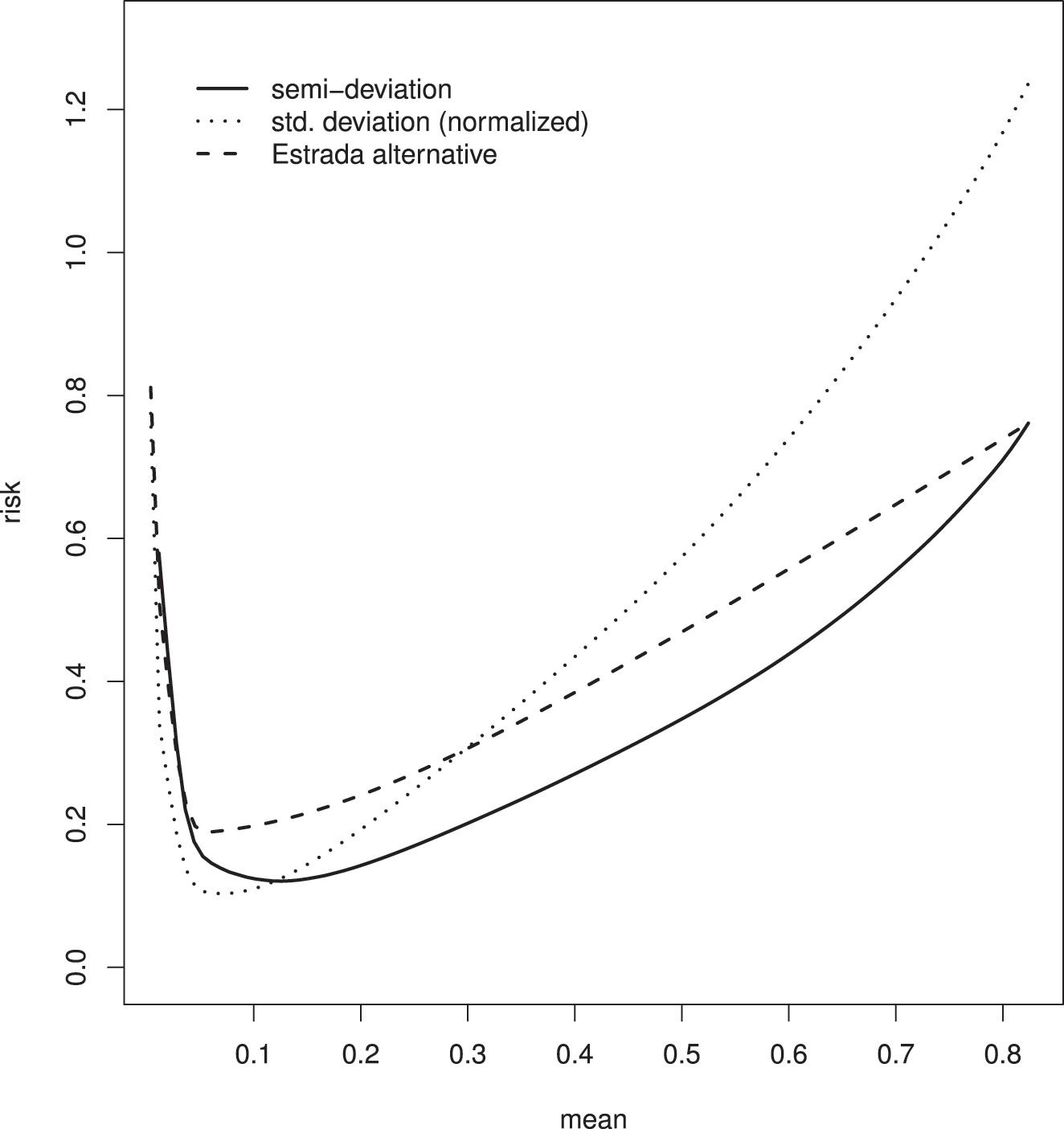
The values of the semi-deviation γ ̄ for these three vectors of weights are respectively 0.429, 0.132, and 0.761. More generally, the value of the semi-deviation γ ̄ for the vector w of weights associated with each of the points on each of the three efficient frontiers is as depicted graphically in Figure 2. Among other things, Figure 2 suggests that the values of w associated with the points on the efficient frontier pertaining to the case where the measure of risk is the standard deviation σ ̄ are similar to those associated with the efficient frontier pertaining to the case where the measure of risk is the semi-deviation γ ̄ .

Figure 2:

Plot (as a function of μ ̄ ) of the semi-deviation γ ̄ for the values of w associated with the points on the efficient frontier in each of 3 cases:  that where the measure of risk is the standard deviation σ ̄ , that where it is the semi-deviation γ ̄ itself, and that where it is the Estrada alternative γ ̃ .

References

Bailey, D. H., and M. López de Prado. 2013. “An Open-Source Implementation of the Critical-Line Algorithm for Portfolio Optimization.” Algoritnms 6: 169–96. https://doi.org/10.3390/a6010169.Suche in Google Scholar
Berkowitz, J. P., C. A. DepkenII, and J. M. Gandar. 2018a. “Exploiting the ‘Win but Does Not Cover’ Phenomenon in College Basketball.” The Financial Review 53: 185–204. https://doi.org/10.1111/fire.12155.Suche in Google Scholar
Berkowitz, J. P., C. A. DepkenII, and J. M. Gandar. 2018b. “The Conversion of Money Lines into Win Probabilities: Reconciliations and Simplifications.” Journal of Sports Economics 19: 990–1015. https://doi.org/10.1177/1527002517696957.Suche in Google Scholar
Britten-Jones, M. 1999. “The Sampling Error in Estimates of Mean-Variance Efficient Portfolio Weights.” The Journal of Finance 54: 655–71. https://doi.org/10.1111/0022-1082.00120.Suche in Google Scholar
Estrada, J. 2008. “Mean-Semivariance Optimization: A Heuristic Approach.” Journal of Applied Finance 18: 57–72.10.2139/ssrn.1028206Suche in Google Scholar
Fishburn, P. C. 1977. “Mean-Risk Analysis with Risk Associated with Below-Target Returns.” The American Economic Review 67: 116–26.Suche in Google Scholar
Harville, D. A. 2020. College Football Ratings and Predictions. Available at https://davidharville.com/collegefootballratingspredictions.Suche in Google Scholar
Lai, T. L., H. Xing, and Z. Chen. 2011. “Mean-Variance Portfolio Optimization when Means and Covariances Are Unknown.” Annals of Applied Statistics 5: 798–823. https://doi.org/10.1214/10-aoas422.Suche in Google Scholar
Levitt, S. D. 2004. “Why Are Gambling Markets Organised So Differently from Financial Markets?” The Economic Journal 114: 223–46. https://doi.org/10.1111/j.1468-0297.2004.00207.x.Suche in Google Scholar
Markowitz, H. M. 1952. “Portfolio Selection.” The Journal of Finance 7: 77–91. https://doi.org/10.1111/j.1540-6261.1952.tb01525.x.Suche in Google Scholar
Markowitz, H. M. 1959. Portfolio Selection: Efficient Diversification of Investments. New York: Wiley.Suche in Google Scholar
Markowitz, H. M. 1987. Mean-Variance Analysis in Portfolio Choice and Capital Markets. Cambridge: Basil Blackwell.Suche in Google Scholar
Markowitz, H. M., D. Starer, H. Fram, and S. Gerber. 2020. “Avoiding the Downside: A Practical Review of the Critical Line Algorithm for Mean-Semivariance Portfolio Optimization.” In Handbook of Applied Investment Research, edited by J. B. Guerard, and W. T. Ziemba, 369–415. Singapore: World Scientific Publishing Company. (Chapter 16).10.1142/9789811222634_0017Suche in Google Scholar
Markowitz, H. M., P. Todd, G. Xu, and Y. Yamane. 1992. “Fast Computation of Mean-Variance Efficient Sets Using Historical Covariances.” Journal of Financial Engineering 1: 117–32.Suche in Google Scholar
Markowitz, H. M., P. Todd, G. Xu, and Y. Yamane. 1993. “Computation of Mean-Semivariance Efficient Sets by the Critical Line Algorithm.” Annals of Operations Research 45: 307–17. https://doi.org/10.1007/bf02282055.Suche in Google Scholar
Niedermayer, A., and D. Niedermayer. 2010. “Applying Markowitz’s Critical Line Algorithm.” In Handbook of Portfolio Construction: Contemporary Application of Markowitz Techniques, edited by J. B. Guerard, 383–400. New York: Springer. (Chapter 12).10.1007/978-0-387-77439-8_12Suche in Google Scholar
© 2023 the author(s), published by De Gruyter, Berlin/Boston
This work is licensed under the Creative Commons Attribution 4.0 International License.
Artikel in diesem Heft
- Frontmatter
- Research Articles
- Predicting elite NBA lineups using individual player order statistics