Combination of PSInSAR and GPS for stress and strain tensor estimation in Afar

Andnet Nigussie; Mehdi Eshagh; Andenet Ashagrie

doi:10.1515/jogs-2022-0162

Article Open Access

Combination of PSInSAR and GPS for stress and strain tensor estimation in Afar

Andnet Nigussie , Mehdi Eshagh and Andenet Ashagrie

Published/Copyright: February 12, 2025

Published by

Become an author with De Gruyter Brill

Author Information

From the journal Journal of Geodetic Science Volume 15 Issue 1

Abstract

This article investigates the strain and stress tensors of the Afar region using the integration of global navigation satellite system (GNSS) and persistent scatterer interferometric synthetic aperture radar (PSInSAR) data. We first estimated the three-dimensional displacement field of the Afar area using combined GPS and PSInSAR data for the period 2006–2009. Secondly, the variance component estimation is applied to the heterogeneous GNSS and PSInSAR data and the displacement field is computed. Then, the behaviour of crustal movement within the study area is investigated by dividing the region into several small triangles or tetrahedrons using the Delaunay triangulation and applying the finite element method (FEM) to estimate the strain and stress tensors for each tetrahedron. The average stress tensor elements τ x x , τ y y , and τ z z of the study area are 0.067, 0.121, and 0.126 MPa in the North, East, and Up coordinates, respectively. The result also shows that the nearby post-diking deformation has been followed by the Afar Tectono-Magmatic Event that happened in September 2005.

Graphical abstract

Keywords: finite elements; global navigation satellite system; persistent scatterer interferometric synthetic aperture radar; strain; stress

MSC 2010: 65N30; 62J99; 86-08

1 Introduction

The separation of the Nubia, Arabia, and Somalia plates has created Afar 30 Ma years ago (Courtillot 1980, Ebinger et al. 2010). The East African Rift, the Red Sea, and the Gulf of Aden are major structures that make extensions along the three rift branches. The surface displacement in some parts of the Main Ethiopian Rift (MER), is due to a succession of magmatic rift segments where there is an active volcano and tectonic structure in the area, (Pagli et al. 2012, Wright et al. 2012). This surface displacement rate and strain field give an essential constraint on geodynamic models of tectonic movement and in the assessment of earthquake hazards (Walters et al. 2011). Several geodetic measurement methods including global navigation satellite system (GNSS), Interferometric synthetic aperture radar (InSAR), are currently applied to measure surface deformation (Norin et al. 2018). GNSS provides absolute three-dimensional (3D) dynamic changes of surface deformation information, considering the coordinates of surveyed points. GPS data give higher precision displacements vector at higher temporal sampling rates and a moderate spatial sampling (10 km) but it cannot describe deformation spatial variations in the near-fault area because of its sparse observations.

Surface displacement caused by landslides, glacier movements, land subsidence, earthquakes, and volcanic eruptions can be monitored using InSAR (Miao et al. 2021). InSAR performs monitoring the rate and dispersion of interseismic strain accumulation with a large number of satellite data volumes (Elliott et al. 2008, Wang and Wright 2012) in Northwestern Tibet (Tong et al. 2013, Jin and Funning 2017), the San Andreas fault system (Kaneko et al. 2013), the Anatolian Fault system (Jolivet et al. 2013, Daout et al. 2016), and the Haiyuan fault system in the north-eastern margin of the Tibetan Plateau. Both GNSS and InSAR are extremely complementary methods for monitoring crustal displacement (Wei et al. 2010).

So far a large number of researchers integrated GNSS and InSAR data for different purposes such as investigating infrastructures (Bakon et al. 2014, Tapete et al. 2015, Del Soldato et al. 2021); tectonic and seismic investigation (Farolfi et al. 2019, Wilkinson et al. 2017); uplift and subsidence monitoring (Tomás et al. 2014, Heimlich et al. 2015); seismic distractions in infrastructure and loss in human life in the urban area (Suga et al. 2001); volcanic deformation (Sandwell et al. 2008); post-seismic deformation (Johanson et al. 2006); crustal deformation velocity and strain rate field estimation (Song et al. 2019); to optimally monitor crustal deformation (Chlieh et al. 2004, Nishimura et al. 2008, Decriem and Árnadóttir 2012, Gahalaut et al. 2017).

Different models were used for estimating 3D displacement vectors from combined GNSS and InSAR data. Weighted least squares (WLS) model with variance component estimations [(VCEs) see e.g. Hu et al. (2012) or Mehrabi et al. (2019)]. Houseman and England (1986) applied the finite element method (FEM) to determine strain and stress rates in a thin viscous sheet, representing the continental lithosphere. They showed the relationship between the displacement rate field, the distribution of crustal thickness, stress, and strain rate index. Kiamehr and Sjöberg (2005) investigated the three-dimensional FEM to analyse the surface deformation patterns of the Skåne area in Sweden based on GNSS data. The existing methods, while useful, have limitations in fully capturing the intricacies of deformation patterns in the area. They do not optimally weight the data and simply using VCE and optimally reweight the data to obtain a better and more realistic optimal estimation for the displacement fields, and after that, FEM is used to estimate the stress and strain tensors incorporating geophysical information of the study area obtained from seismic data.

In this article, we apply persistent scatterer interferometric synthetic aperture radar (PSInSAR) and GNSS data for crustal deformation monitoring in the Afar region, Ethiopia. We first combine PSInSAR and GNSS displacement data using least-squares with iterative VCE. After that, the FEM is then applied to estimate the strain and stress model from the combined displacement field to analyse the deformation pattern of the study area.

2 Theory

In this section, we present the mathematical model for combining the line-of-sight (LOS) displacement of ascending and descending InSAR data with GNSS time series data to estimate the strain tensor using FEM.

2.1 GNSS and PSInSAR combination model

One-dimensional (1D) surface displacement d _los in the LOS direction can be obtained by using Permanent Scattering InSAR. In order to derive 3D displacements in the northeast-up (NEU) coordinate system, we need to use other geodetic data such as GNSS with the LOS data. The LOS displacement velocities v LOS of a point can be expressed in terms of velocity components in the NEU system by:

(1a) v LOS = [ v E v N v U ] [ e E e N e U ] T ,

where v E , v N , and v U are the eastward, northward, and upward components of the velocity vector and e E , e N , and e U are the unit vectors of the NEU system. []^T stands for the transpose operator. These unit vectors have the following relationship with θ i nc is the incidence angle of satellite sight, and α h is the heading angle, that is, the clockwise angle between the north and the flight of the satellite.

(1b) [ e E e N e U ] T = [ − sin θ i nc cos α h sin θ i nc sin α h cos θ i nc ] .

The three-dimensional displacement field is calculated using the observation equations equation (2a) of the least-squares model on the interpolated GNSS and PSInSAR observations ascending and descending observation.

(2a) A x = L + v , E { v } = 0 and E { v v T } = σ 0 2 Q = ∑ i = 1 q σ i 2 Q i ,

where E { } is the statistical expectation, v is vector of random errors, Q the co-factor matrix, σ 0 2 the a priori variance factor, σ i 2 variance component of the ith set of data with the co-factor matrix Q _i. Q is the total number of variance components. The structures of A, x, and L are:

(2b) A = − sin θ ASC cos α ASC sin θ ASC sin α ASC cos θ ASC − sin θ DES cos α DES sin θ DES sin α DES cos θ DES 1 0 0 0 1 0 0 0 1 , x = v E v N v U and L = v LOS ASC v LOS DES v E GPS v N GPS v U GPS ,

where v LOS ASC and v LOS DES are, respectively, the LOS velocities of ascending and descending tracks of the satellites. v E GPS , v N GPS , and v U GPS are the velocity of displacement derived from GNSS in the NEU system. To determine the displacement velocities, a WLS method is applied (Hu et al. 2012):

(2c) x ˆ = ( A T Q − 1 A ) − 1 A T Q − 1 L .

It is self-evident that the choice of the a priori variance factor does not affect the estimated parameters. However, the precision of the input data has a significant impact on the results of a least-squares process. Data with higher precision contribute more to the estimates than those with lower precision. The critical question is how realistic the data precision is. It can be unrealistically high, causing the solutions to be skewed towards such data, even if their inherent quality is not that high. In such cases, a reweighting scheme is necessary to balance the data precision with the precision of the least-squares process. Such methods are commonly referred to as VCE.

2.2 VCE

In this study, we divided our observations to three groups and update the weight matrix of the observations iteratively using the VCE. Assuming that L 1 , L 2 , and L 3 are, respectively, the three observation groups of the PSInSAR LOS velocities, the vertical and horizontal GNSS velocities, and P 1 , P 2 , and P 3 their corresponding weight matrices, three sets of residuals can be estimated after the solution given in equation (3a).

(3a) v ˆ i = A i x ˆ − L , i i = 1 , 2 , and 3 .

The vector of variance components can be derived by solving the following system of equations

(3b) r ˆ = S VC − 1 w R ,

where

(3c) r ˆ = σ ˆ 1 2 σ ˆ 2 2 σ ˆ 3 2 T ,

is vector of variance components and

(3d) w R = [ v ˆ 1 T P 1 v ˆ 1 v ˆ 2 T P 2 v ˆ 2 v ˆ 3 T P 3 v ˆ 3 ] T ,

(3e) S VC = m − 2 tr ( N − 1 N 1 ) + tr ( N − 1 N 1 ) 2 tr ( N − 1 N 1 N − 1 N 2 ) tr ( N − 1 N 1 N − 1 N 3 ) tr ( N − 1 N 1 N − 1 N 2 ) m − 2 tr ( N − 1 N 2 ) + tr ( N − 1 N 2 ) 2 tr ( N − 1 N 2 N − 1 N 3 ) tr ( N − 1 N 1 N − 1 N 3 ) tr ( N − 1 N 2 N − 1 N 3 ) 2 m − 2 tr ( N − 1 N 3 ) + tr ( N − 1 N 3 ) 2 ,

where

(3f) N i = A i T P i A i and N = ∑ i = 1 3 A i T P i A i ,

(3g) P = P 1 0 0 0 P 2 0 0 0 P 3 and A = A 1 A 2 A 3 ,

where A 1 , A 2 , and A 3 are, respectively, the coefficients matrices of the first, second, and third set of observations with weight matrices of P 1 , P 2 , and P 3 .

The new weight matrices are then determined from the VC.

(3h) P ˆ 1 = P 1 ,

(3i) P ˆ 2 = σ ˆ 1 2 σ ˆ 2 2 P 2 ,

(3j) P ˆ 3 = σ ˆ 1 2 σ ˆ 3 2 P 3 .

where P 1 , P 2 , and P 3 are replaced by P ˆ 1 , P ˆ 2 , and P ˆ 3 , and the WLS process and VCE are repeated until σ ˆ 1 2 = σ ˆ 2 2 = σ ˆ 3 2 .

2.3 Strain and stress

Tectono-magmatic activities exert a force on the rock of the earth causing deformation over different areas. Stress and strain are tools for studying the deformable Earth. Mathematically strain is defined as the change of the displacement with respect to its position. Consider that the displacement vector at a point with the position ( x , y , z ) in the NEU system is presented by

(4a) s ( x , y , z ) = ( α , β , γ ) ,

where ( α , β , γ ) are displacement components.

The strain tensor is defined as:

(4b) ε = ∂ s ∂ x = ∂ α ∂ x ∂ α ∂ y ∂ α ∂ z ∂ β ∂ x ∂ β ∂ y ∂ β ∂ z ∂ γ ∂ x ∂ γ ∂ y ∂ γ ∂ z .

The displacement components at the point i can be derived from the position and strain tensor by:

(4c) α i β i γ i = ε x x ε x y ε x z ε x y ε y y ε y z ε x z ε y z ε z z x i y i z i + 0 ω z ω y − ω z 0 ω x − ω y − ω x 0 x i y i z i ,

where ( ε x x , ε y y , and ε z z ) and ( ε x y , ε y z , and ε x z ) are unknown normal strain tensor and shear strain tensor deformation parameters, respectively, and ω i , i = x, y, z are the rotational deformations round x, y and z directions at each point.

Equation (4c) consists of three equations for the displacement and by considering the elements of the strain tensor are unknown at point i, equation (4c) is rearranged in the following form:

(4d) α i β i γ i = x i 0 0 y i 0 z i 0 z i y i 0 y i 0 x i z i 0 z i 0 − x i 0 0 z i 0 y i x i − y i − x i 0 ε x x ε y y ε z z ε x y ε y z ε x z ω x ω y ω z .

Equation (4d) is a system of three equations and nine unknowns and as such has infinitely many solutions. Therefore, at least two more points are needed to have nine equations and a unique solution, and in the case of having more, the least-squares method can be applied to solve the parameters. Here, the FEM is used meaning that the area or the deformable object is divided into small pieces, or finite elements (FEs), having with own strain tensors. Let us consider all points of a piece in one system of equations with the following form

(5a) d = B e ,

where d is the vector of one vertex, e is the vector matrix of deformation parameters, and B is the coefficient matrix of deformation parameters.

Assuming the strain is uniformly spread all over the deformable object, the area of study is divided into FEs where the strain components are constant. We chose triangles or tetrahedrons of geodetic benchmarks using the Delaunay triangulation. The area of interest is divided into small triangular FEs; e.g. in this study 21,070FEs of tetrahedron shape are formed. One may associate the illustrated tetrahedron in Figure 1 with any of those elements.

Figure 1

A tetrahedron as a three-dimensional FE.

In Figure 1, the vertices of the tetrahedron a, b, c, and d represent any four irregularly located points in the network, which forms an FE according to the Delaunay optimal conditions. To determine six unknown strain components three equations are formed for each vertex of the FE and since there are four vertices, 12 equations are created for solving the nine unknown strain components. Let us rewrite equation (5a) in the following form:

(5b) D + v ′ = K B e ,

where D stands for the vector of displacements of all four vertices:

(5c) D = d x a d y a d z a d x d d x d d x d T ,

is a vector observation; v′ is the residual vector, K is a design matrix element specifying which vertices should be connected to each other and since we have six lines for each FE then this design matrix has 6 × 3 rows and based on the four vertices 4 × 3 columns:

(5d) K = − 1 0 0 1 0 0 0 0 0 0 0 0 0 − 1 0 0 1 0 0 0 0 0 0 0 0 0 − 1 0 0 1 0 0 0 0 0 0 ⋮ 0 0 0 0 0 0 − 1 0 0 1 0 0 0 0 0 0 0 0 0 − 1 0 0 1 0 0 0 0 0 0 0 0 0 − 1 0 0 1 18 × 12 .

B is the coefficient matrix of the deformation model equation (4d):

(5e) B = x a 0 0 y a 0 z a 0 z a y a 0 y a 0 x a z a 0 z a 0 − x a 0 0 z a 0 y a x a − y a − x a 0 ⋮ x d 0 0 y d 0 z d 0 z d y d 0 y d 0 x d z d 0 z d 0 − x d 0 0 z d 0 y d x d − y d − x d 0 12 × 9 ,

and finally

(5f) e = ε x x ε y y ε z z ε x y ε x z ε y z ω x ω y ω z T .

The least-squares solution of equation (5d) is (Alizadeh Khameneh et al. 2018):

(5g) e ˆ = ( B T K T K B ) − 1 B T K T K D .

The variance–covariance matrix of the estimated deformation parameters for each FE is:

(5h) C e ˆ = ( B T K T K B ) − 1 B T K T K C D K T K B ( B T K T K B ) − 1 .

Finally, we estimated the strain tensor for each block element. From a linear elasticity theory, the stress tensor elements can directly be calculated from the strain tensor elements (Eshagh et al. 2020).

We have computed the divergence of the displacement vectors using the CRUST1.0 model and the given elasticity parameters determined by the seismic velocities.

The mathematical relationship is

(6a) τ i j = δ i j γ ∇ ⋅ s + μ ε i j ,

where i , j = x, y, and z. γ and μ are elasticity parameters that describe the mechanical properties of a material, δ i j is the Kronecker delta and ∇·s is the divergence of displacement vectors, and τ x x , τ y y , and τ z z are the normal stress tensor elements; and τ x y , τ x z , and τ y z are the shear stress tensor elements. The divergence of the displacement vector ( ∇ ⋅ s ) is calculated based on equation (4d) where the divergence of the displacement vector is equal to the trace of the diagonal stain tensor for normal stress components and zero for shear stress components. The γ and μ elasticity parameters are extracted from CRUST1.0 model of the top surface (Laske et al. 2013).

3 Study area and its tectonic setting

The area is located in the North-East African Rift valley and is among the seismically active regions of the earth. It covers five districts of the Afar regional states, namely Ewa, Gulina, Habru, Teru, and Yalo (Figure 2). In these areas, we found the 4 years of GNSS and PSInSAR data.

Figure 2

Map of the study area. The blue dots are GNSS stations with five districts of the Afar regional state.

In Afar, nucleation of the rock was taken place by thermal anomalies related to mantle plumes that cause weakening of the lithosphere and strain locations (Bellahsen et al. 2003). The main causes of tectonics are normal faults and open fissures (Abbate et al. 1995). These faults and volcanoes cover ∼60 km length and ∼10 km width segments with aligned chains of basaltic cones (Ayele et al. 2009). The uplift and subsidence in response to magmatic intrusions, or to the tectonic extension are spread over the area (Saria et al. 2013). The Dabbahu magmatic segment (DMS) trends NW-SE from the area of Ado’Ale and to the south, and it trends to the north, in a more northerly direction. At the northern end, there are many active volcanoes including the Dabbahu and Gab’ ho. A DMS segment is ∼60 km long and 15 km wide area which has been a place of the volcano-tectonic episode during 2005–2010 (e.g., Ebinger et al. 2010). The narrow, large faults and fissures of the rift axis are flanked on both sides by silicic volcanoes forming the Ado’Ale Volcanic Complex to the east, and the west (Ayele et al. 2009). The present study confirms that the frequency of crustal deformation of the type observed at the Dabbahutectono-magmatic activities in 2005 can create strain and stress in the area.

4 Result

In this section, the results of GNSS and PSInSAR data combination using VCE, the strain tensor element, and the stress tensor element of the Afar area obtained by integrated GNSS and PSInSAR displacement are presented.

4.1 GNSS and PSInSAR data combination using VCE

The PSInSAR and GNSS data were combined using equation (2b). Initially, it was assumed that the variance of GNSS is the same as the variance of PSInSAR for the first iteration. An algorithm was used to estimate the variance of the parameters for each GNSS station, as shown in Table 1. The results show the combined velocities in the East, North, and Up directions, revealing that land deformation is dominantly characterized by a northward movement or displacement, which can be the result of tectonic plate interactions.

Table 1

Statistics of error before and after VCE (mm/year)

GPS stations	σ _GPS			σ _PSInSAR		After
GPS stations	σ _E	σ _N	σ _U	σ _A	σ _D	σ _E	σ _N	σ _U
DA25	0.16	0.82	0.45	0.92	0.62	0.22	0.31	0.02
DA35	0.17	0.54	0.49	0.96	0.58	0.55	0.08	0.01
DA45	0.16	0.25	0.23	0.93	0.59	0.23	0.20	0.04
DA60	0.08	0.09	0.20	0.91	0.57	0.17	0.06	0.01
DABB	1.26	1.20	3.00	0.90	0.59	0.96	0.74	1.21
DABT	0.08	0.10	0.29	0.95	0.58	0.64	0.01	0.31
DATR	0.16	0.58	0.46	0.93	0.58	0.52	0.09	0.02

Table 1 provides important information regarding the estimated standard deviations for each GNSS station before and after VCE. The standard deviations of the estimated parameters are denoted by σ E , σ N , and σ U for the East, North, and Up directions, respectively. The columns σ GNSS and σ PSInSAR display the variance before the estimation process in the three directions. After VCE, the standard deviations are depicted in the last three columns, indicating smaller results compared to the standard deviation values before VCE.

The table also shows that the errors before and after a combination of InSAR and GNSS data are generally in good agreement, except for the DABB station, which has a large variation due to the unavailability of sufficient GNSS data during the study period. However, the combination of PSInSAR and GNSS data provides a reliable estimate of the velocity in most cases.

The velocity difference between the East, North, and Up directions before and after VCE was included in the table. The maximum error of 33 mm/year is observed in the DABB station, which is consistent with the large variation mentioned earlier. This indicates that the VCE method is suitable for uncertainty investigation.

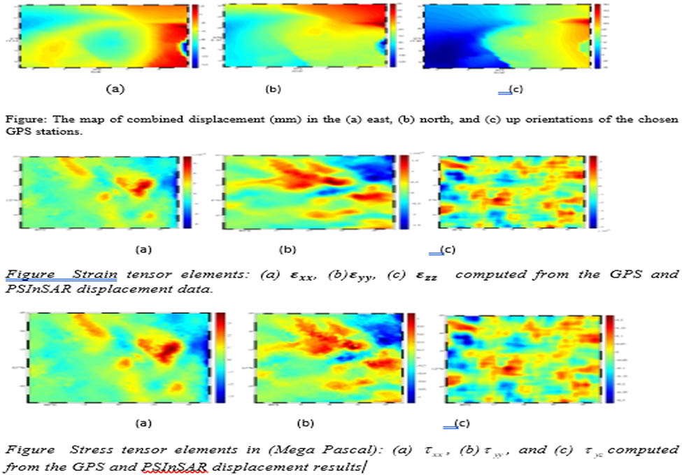
The velocities in the East, North, and Up directions, combined with the PSInSAR and GNSS data, are, respectively, displayed in Figure 3a–c. Figure 3a provides valuable insights into the combined velocity of the study area, measured in the East direction. This movement is a manifestation of tectonic processes taking place beneath the Earth’s surface, including continental drift and plate motion. The displacement, measured in millimetres, offers crucial information regarding the rate at which the land is moving and deforming over time, which can be instrumental in predicting future geological changes. The diagram displays a range of velocity between −40 and 60 mm/year, indicating that the area is experiencing a moderate level of movement and deformation.

Figure 3

The map of combined displacement (mm) in the (a) east, (b) north, and (c) up directions of the selected GNSS stations.

The observed velocity of 60 mm/year encountered around the DABB station, and the velocity of −40 mm/year, encountered around the DA25 station, can be explained by the presence of geological faults in the area. These faults are the places where the Earth’s crust has been broken, leading to the formation of blocks that can move in different directions. The differences in velocity at the DABB and DA25 stations suggest that the blocks on either side of the faults are moving relative to each other at different rates and directions.

In addition to the East direction, Figure 3b shows the combined displacement map in the North direction. The range of velocity is between 1 and 90 mm/year around DABB and DA45 GNSS stations respectively. This information can offer important clues about the tectonic processes that play in the area and the resulting deformation patterns.

Figure 3c displays the combined displacements in the Up direction, with a maximum uplift of approximately 160 mm observed around the DA25 GNSS station and a maximum subsidence of −40 mm around the DABT GNSS station. This information is crucial for understanding the vertical movement of the land and related geological processes like uplift and subsidence. Figure 3a–c offer valuable insights into the intricate tectonic processes happening beneath the Earth’s surface and can aid in predicting future geological changes. The results reveal that the movement of the land in the study area is increasing, which highlights the need for necessary precautions to mitigate the geo-hazard in the area.

Figure 4 illustrates the variance components’ ratios during the iterative VCE process. It demonstrates a descending pattern, commencing at a significant displacement variance and aligning with two iterations. The convergence of iterations occurs around the fourth iteration.

Figure 4

The plot of variance components ratios’ behaviour during the iteration and their convergence.

4.2 Strain tensor and stress tensor

Figure 5a–f illustrates the strain tensor elements computed from the combination of 3D GNSS velocities and PSInSAR LOS velocities gathered from 2006 to 2009, showing minimum values of ε x x , ε y y , and ε z z , (−6.9 × 10⁻⁶, −1.2 × 10⁻⁶, and −2.3 × 10⁻⁵) strain/year, and maximum value of ε x x , ε y y , and ε z z , (7.4 × 10⁻⁶, 1.03 × 10⁻⁶, and 5.43 × 10⁻⁵) strain/year respectively. Some residual deformation largely near Ado Ale and Dabbahu volcanoes is credited to a meshing size that is likely too large-grained to precisely repeat focused signals at volcanoes. We observed dominant strain tensor and stress tensor elements near Dabbahu, which can possibly be the occurrence of the nearby post-diking deformation of 2005. This deformation spreads up to a 200-km-wide area overlapping many rift segments as Pagli et al. (2014) also pointed out. Uplift subsidence was observed as a result of the continuous flow of magma. This is in good agreement with the previous research study results (Hamling et al. 2014, Pagli et al. 2014), indicating that the transit post-diking deformation around Dabbahu is the cause of the strain. The continuous magma flows from the distinct portion of the segment to the Ado Ale chamber in the rift also contributes to the deformation detected in the area.

$Figure 5 Strain tensor elements: (a) ε x x {\varepsilon }_{xx} , (b) ε y y {\varepsilon }_{yy} , (c) ε z z {\varepsilon }_{zz} , (d) ε x y {\varepsilon }_{xy} , (e) ε x z {\varepsilon }_{xz} , and (f) ε y z {\varepsilon }_{yz} computed from the GNSS and PSInSAR displacement results.$

Figure 5

Strain tensor elements: (a) ε x x , (b) ε y y , (c) ε z z , (d) ε x y , (e) ε x z , and (f) ε y z computed from the GNSS and PSInSAR displacement results.

As we expected our estimated displacement fields agree with those published so far, Pagli et al. (2014) used high-resolution data and employed a 3D velocity field analysis, providing extensive spatial coverage and real-time assessment of displacements. Although our research covers the same area and time frame as Pagli et al.’s (2014) studies, our investigation differs from Pagli et al.’s (2014) in several respects. We provide a clear description of the methodology for combining GNSS and PSInSAR data, utilizing variance component analysis. Additionally, we estimate the strain tensor using the finite element method and derive the stress tensor from the strain tensor, incorporating the theory of elasticity.

Furthermore, our study employs PSInSAR, emphasizing a unique methodology focused on determining three-dimensional crustal deformation through VCE to properly weigh the data. This approach, not applied by Pagli et al. (2014), has enabled us to achieve optimal estimations, capturing deformation patterns near fault areas with a level of detail that was previously challenging using conventional methods.

Most importantly, our objective is to present the stress and strain regimes over the study area. To achieve this, we have incorporated the 3D finite element method, which represents a novel approach to the study.

Figure 6a–c depicts the rotational strain elements along the tensor components ω x x , ω y y and ω z z . These rotational deformation estimates manifest the values spanning the magnitude range of −1 × 10⁻⁴ to 1.5 × 10⁻⁴, −1 × 10⁻⁴ to 1 × 10⁻⁴, and −4 × 10⁻⁴ to 2 × 10⁻⁴ within the East, North, and Up directions, respectively. This portrayal is indicative of the dynamic movement of medium tectonic plates and consequential seismic activities that transpire within the study area.

$Figure 6 Rotational Strain tensor elements (rad/year): (a) ω x x {\omega }_{xx} , (b) ω y y {\omega }_{yy} , and (c) ω z z {\omega }_{zz} , computed from the GNSS and PSInSAR displacement results.$

Figure 6

Rotational Strain tensor elements (rad/year): (a) ω x x , (b) ω y y , and (c) ω z z , computed from the GNSS and PSInSAR displacement results.

The largest value of the stress tensor is detected in Figure 7a revealing the highest magnitude of the stress tensor, while the mean stress tensor components amount to 0.121 MPa in the East, 0.067 MPa in the North, and 0.126 MPa in the Up directions. The larger expansion of the stress tensor element τ x x across the Dabbahu region can be attributed to the proximate post-diking deformation that followed the Afar Tectono-Magmatic Event of September 2005. The observations also exhibit substantial similarity to the stress analysis conducted by Gedamu et al. (2023).

$Figure 7 Stress tensor elements in (Mega Pascal): (a) τ x x {\tau }_{xx} , (b) τ y y {\tau }_{yy} , (c) τ z z {\tau }_{zz} , (d) τ x y {\tau }_{xy} , (e) τ x z {\tau }_{xz} and (f) τ y z {\tau }_{yz} computed from the GNSS and PSInSAR displacement results.$

Figure 7

Stress tensor elements in (Mega Pascal): (a) τ x x , (b) τ y y , (c) τ z z , (d) τ x y , (e) τ x z and (f) τ y z computed from the GNSS and PSInSAR displacement results.

The findings of this study indicate a predominant NW-SE orientation for the maximum horizontal stress and an NE-SW orientation for the minimum horizontal stress within the region. Moreover, the researchers also observed localised extensional deformation in the study area, proposing a likely correlation with intrusive diking activities in line with the work. Our findings harmonize with Hamling et al.’s (2009) outcomes, reinforcing the inference that stress redistribution in the study area can be attributed to the diking event.

The spatial distributions of shear strain tensor elements ( ε x x , ε y y , and ε z z ) and normal strain tensor elements ( ε x x , ε y y , and ε z z ), along with the corresponding spatial patterns of shear stress tensor elements ( τ x x , τ y y , and τ z z ) and normal stress tensor elements ( τ x x , τ y y , and τ z z ) computed from the combined 3D GNSS and PSInSAR displacement field results are illustrated in Figures 5d–f and 7d–f, respectively.

Since the area of study is small, the comparative analysis between the spatial patterns of shear strain tensor ε x y and shear stress tensor elements τ x y reveals a notable degree of similarity. However, the strain tensor elements presented in Figure 5e and f diverge from the stress tensor elements displayed in Figure 7e and f. This divergence is attributed to observed non-uniform horizontal displacement along the Dabbahu region, which gradually attenuates towards the segment boundaries.

In this experimental section, we delve into the unique findings and advantages of our research approach in the context of the Afar region’s complex geological dynamics. Our study has unveiled several key insights that contribute to a deeper understanding of crustal deformation in this region.

Firstly, by combining PSInSAR and GNSS data in a least-squares sense and using VCE we have optimally weighted data, which was not applied so far over this study area. In this case, more optimal displacements can be estimated rather than a simple combination method using an ordinary least-squares method. Having realistic and optimal displacement fields is of vital importance for deformation analysis to capture the patterns in near-fault areas with a level of detail that was challenging for previous methods. In addition, applying PSInSAR and GNSS data for determining stress and strain tensors through the FEM is a novel application over this study data. This advancement is critical for assessing earthquake hazards and understanding tectonic movements in the Afar region.

5 Discussion

In this study, the spatial trend of strain and stress tensor elements of the Afar area was determined with the combined GNSS and PSInSAR displacement results. We get maximum normal strain rate ( ε x x ) and shear strain rate ( ε x y ) respectively, 0.74 × 10⁻⁷ and 0.1 × 10⁻⁷ during the same observation time which is the result of the post-diking process. The 2005 rifting episode of Afar happened by a large magma intrusion (2–2.5 km³). Bernie et al. (2016) in their study showed that the maximum horizontal stress in the Afar region is oriented NW-SE and the minimum horizontal stress is oriented NE-SW which is similar to our study results. We suggest that a continuous superimposed accelerated spreading of magma flow from a distant part of the segment towards the Ado Ale chamber in the rift centre occurs, contributing to this strain (Hamling et al. 2014). The research work by Hamling et al. (2009) found that the intrusion of a dyke causes stress transfer to the surrounding area, leading to localised deformation and uplift. The magnitude and orientation of the stress transfer were found to vary depending on the orientation and position of the dyke relative to other dykes and faults in the region. They also identified variations in the strength and orientation of the crustal stress field over time, indicating a complex and dynamic tectonic regime in the region. Ebinger et al. (2010) showed variations in the composition and properties of magma at different stages of the rifting process, suggesting that magma evolution is influenced by changes in tectonic and thermal conditions in the crust this result to cause the stress and strain tensor in the area. Barnie et al. (2016) found that the crustal stress field in the MER is characterized by a dominant NNE-SSW compression, consistent with the regional tectonic regime.

The reason for the presence of subsidence and uplift in both the south (around Semera) and the north (around Dabbahu–Manda–Hararo) could be attributed to the existence of shallow magma chambers and a deep magma chamber in the respective areas. The stress release due to dyke intrusion resulted in the associated subsidence in one of the areas magma might be depleted from the chamber in the other area to cause uplift. The deformation pattern depicted a higher uplift in the northern part where stations DABB are found.

Overall, the findings contribute to a better understanding of the complex mechanisms of magmatic activity. This has important implications for assessing volcanic hazards and understanding the tectonic processes underlying continental rifting, as well as the mechanisms of stress transfer and deformation in the Afar region. These findings are consistent with the results of other researchers who have conducted studies in the study area.

6 Conclusion

In conclusion, the article has provided unique insights and advantages within the intricate geological dynamics of the Afar region. Through our research, we have uncovered key findings that significantly enhance our comprehension of crustal deformation in this area.

First and foremost, our innovative approach combines PSInSAR and GNSS data using a least-squares method with VCE, a technique previously unutilized in this region. This approach optimally weighs the data, resulting in more accurate displacement estimations compared to conventional methods that rely on ordinary least-squares. The significance of this lies in the capacity to capture detailed displacement patterns, especially in proximity to volcanically active areas, and fault areas, where previous methods fell short.

Furthermore, our use of PSInSAR and GNSS data to determine stress and strain tensors through finite element method (FEM) represents a ground-breaking application for this specific dataset. This advancement is pivotal in evaluating earthquake hazards and gaining insights into the complex tectonic movements occurring in the Afar region.

Overall, our research not only enhances our understanding of crustal deformation in the Afar region but also provides valuable tools and methodologies for future studies in similar geological contexts.

7 Summary

Tectonic and magmatic deformation of the crust results in the establishment of stress and strain over the area. These parameters describe the intensity of crustal deformation, which is used to monitor geodynamic processes and take the necessary precautions to mitigate geodynamic hazards. The deformation of deformable objects can be measured using geodetic measurements. GNSS and PSInSAR are the most widely used geodetic techniques to monitor the surface displacement field. The combination of the two geodetic techniques can provide a high temporal and spatial resolution to measure the three-dimensional displacement field of the ground surface deformation. The strain and stress tensors can also be calculated from the combined 3D displacement field results. This measurement of deformation parameters needs an appropriate model of deformation which must be fitted to the deformation of the area. To measure the displacements, strain, and stress fields; separate network points in different time intervals are taken. From the relationships among the displacement, strain, and stress field variations, the deformation parameters (strain and stress) were estimated.

In a global or regional network (large-scale areas), the behaviour of crustal movement is not the same within the object. Therefore, we have todiscretiseour study area into small sub-areas using FEM. In FEM the region is divided into several small triangles or tetrahedrons, and the approach is Delaunay triangulation. In this study, we first estimated the 3D displacement field of Afar areas using combined GNSS and PSInSAR data between 2006 and 2009. Then, the quality control measures of combined heterogeneous (GNSS and PSInSAR) data were estimated using the VCE method finally, applying the FEM approach, the strain and stress field tensor were calculated and the results showed that the nearby post-diking deformation followed by the Afar Tectono-Magmatic Event that happened in September 2005 mainly affected both the strain and stress tensor elements.

Acknowledgments

We would like to acknowledge ESA and UNAVCO for SAR and GNSS data provision. We appreciate Debre Berhan University for the sponsorship of the Ph.D. study. We are thankful to Doctor Daniele Perisin for providing SARPROZ software.

Funding information: Authors state no funding involved.
Author contributions: Andnet Nigussie Habte: Conceptualization, methodology, analysis, manuscript writing, and overall project supervision. Mehdi Eshagh: Overall research supervision and guidance and Interpretation of results, review, and editing of the manuscript. Andnet Ashagrie Gedamu: Interpretation of results, review, and editing of the manuscript.
Conflict of interest: Authors state no conflict of interest.
Data availability statement: The data used in this study is available from UNAVCO (https://www.unavco.org/) and can be accessed upon request. Further details regarding data sharing and access policies can be found in the Data Sharing Policy document available on the journal’s website.

References

Abbate, E., P. Passerini, and L. Zan. 1995. “Strike-slip faults in a rift area: a transect in the Afar Triangle, East Africa.” Tectonophysics 241(1–2), 67–97.10.1016/0040-1951(94)00136-WSearch in Google Scholar

Ayele, A., D. Keir, C. Ebinger, T. J. Wright, G. W. Stuart, W. R. Buck, E. Jacques, G. Ogubazghi, and J. Sholan. 2009. “September 2005 mega‐dike emplacement in the Manda‐Harraro nascent oceanic rift (Afar depression).” Geophysical Research Letters 36(20), 2–5.10.1029/2009GL039605Search in Google Scholar

Bakon, M., D. Perissin, M. Lazecky, and J. Papco. 2014. “Infrastructure non-linear deformation monitoring via satellite radar interferometry.” Procedia Technology 16, 294–300.10.1016/j.protcy.2014.10.095Search in Google Scholar

Barnie, T. D., D. Keir, I. Hamling, B. Hofmann, M. Belachew, S. Carn, D. Eastwell, J. O. Hammond, A. Ayele, C. Oppenheimer, and T. Wright. 2016. “A multidisciplinary study of the final episode of the MandaHararo dyke sequence, Ethiopia, and implications for trends in volcanism during the rifting cycle.” Special Publications 420(1), 149–63.10.1144/SP420.6Search in Google Scholar

Bellahsen, N., C. Faccenna, F. Funiciello, J. M. Daniel, and L. Jolivet. 2003. “Why did Arabia separate from Africa? Insights from 3-D laboratory experiments.” Earth and Planetary Science Letters 216(3), 365–81.10.1016/S0012-821X(03)00516-8Search in Google Scholar

Chlieh, M., J. B. De Chabalier, J. C. Ruegg, R. Armijo, R. Dmowska, J. Campos, and K. L. Feigl. 2004. “Crustal deformation and fault slip during the seismic cycle in the North Chile subduction zone, from GPS and InSAR observations.” Geophysical Journal International 158(2), 695–711.10.1111/j.1365-246X.2004.02326.xSearch in Google Scholar

Courtillot, V. E. 1980. “Opening of the Gulf of Aden and Afar by progressive tearing.” Physics of the Earth and Planetary Interiors 21(4), 343–50.10.1016/0031-9201(80)90137-5Search in Google Scholar

Daout, S., R. Jolivet, C. Lasserre, M. P. Doin, S. Barbot, P. Tapponnier, G. Peltzer, A. Socquet, and J. Sun. 2016. “Along-strike variations of the partitioning of convergence across the Haiyuan fault system detected by InSAR.” Geophysical Supplements to the Monthly Notices of the Royal Astronomical Society 205(1), 536–47.10.1093/gji/ggw028Search in Google Scholar

Decriem, J. and T. Árnadóttir. 2012. “Transient crustal deformation in the South Iceland Seismic Zone observed by GPS and InSAR during 2000–2008.” Tectonophysics 581, 6–18.10.1016/j.tecto.2011.09.028Search in Google Scholar

Del Soldato, M., P. Confuorto, S. Bianchini, P. Sbarra, and N. Casagli. 2021. “Review of works combining GNSS and InSAR in Europe.” Remote Sensing 13(9), 1684.10.3390/rs13091684Search in Google Scholar

Ebinger, C., A. Ayele, D. Keir, J. Rowland, G. Yirgu, T. Wright, M. Belachew, and I. Hamling. 2010. “Length and timescales of rift faulting and magma intrusion: The Afar rifting cycle from 2005 to present.” Annual Review of Earth and Planetary Sciences 38, 439–66.10.1146/annurev-earth-040809-152333Search in Google Scholar

Elliott, J. R., J. Biggs, B. Parsons, and T. J. Wright. 2008. “InSAR slip rate determination on the AltynTagh Fault, northern Tibet, in the presence of topographically correlated atmospheric delays.” Geophysical Research Letters 35(12), L12309.10.1029/2008GL033659Search in Google Scholar

Eshagh, M., F. Fatolazadeh, and R. Tenzer. 2020. “Lithospheric stress, strain and displacement changes from GRACE-FO time-variable gravity: case study for Sar-e-Pol Zahab Earthquake 2018.” Geophysical Journal International 223(1), 379–97.10.1093/gji/ggaa313Search in Google Scholar

Farolfi, G., A. Piombino, and F. Catani. 2019. “Fusion of GNSS and satellite radar interferometry: Determination of 3D fine-scale map of present-day surface displacements in Italy as expressions of geodynamic processes.” Remote Sensing 11(4), 394.10.3390/rs11040394Search in Google Scholar

Gahalaut, V. K., R. K. Yadav, K. M. Sreejith, K. Gahalaut, R. Bürgmann, R. Agrawal, and A. Bansal. 2017. “InSAR and GPS measurements of crustal deformation due to seasonal loading of Tehri reservoir in Garhwal Himalaya, India.” Geophysical Journal International 209(1), 425–33.10.1093/gji/ggx015Search in Google Scholar

Gedamu, A. A., M. Eshagh, and T. B. Bedada. 2023. “Lithospheric stress due to mantle convection and mantle plume over East Africa from GOCE and seismic data.” Remote Sensing 15(2), 462.10.3390/rs15020462Search in Google Scholar

Hamling, I. J., A. Ayele, L. Bennati, E. Calais, C. J. Ebinger, D. Keir, and G. Yirgu. 2009. “Geodetic observations of the ongoing Dabbahu rifting episode: new dyke intrusions in 2006 and 2007.” Geophysical Journal International 178(2), 989–1003.10.1111/j.1365-246X.2009.04163.xSearch in Google Scholar

Hamling, I. J., T. J. Wright, E. Calais, E. Lewi, and Y. Fukahata. 2014. “InSAR observations of post-rifting deformation around the Dabbahu rift segment, Afar, Ethiopia.” Geophysical Journal International 197(1), 33–49.10.1093/gji/ggu003Search in Google Scholar

Heimlich, C., N. Gourmelen, F. Masson, J. Schmittbuhl, S. W. Kim, and J. Azzola. 2015. “Uplift around the geothermal power plant of Landau (Germany) as observed by InSAR monitoring.” Geothermal Energy 3(1), 1–12.10.1186/s40517-014-0024-ySearch in Google Scholar

Houseman, G. and P. England. 1986. “A dynamical model of lithosphere extension and sedimentary basin formation.” Journal of Geophysical Research: Solid Earth 91(B1), 719–29.10.1029/JB091iB01p00719Search in Google Scholar

Hu, J., Z. W. Li, Q. Sun, J. J. Zhu, and X. L. Ding. 2012. “Three-dimensional surface displacements from InSAR and GPS measurements with variance component estimation.” IEEE Geoscience and Remote Sensing Letters 9(4), 754–8.10.1109/LGRS.2011.2181154Search in Google Scholar

Jin, L. and G. J. Funning. 2017. “Testing the inference of creep on the northern Rodgers Creek fault, California, using ascending and descending persistent scattererInSAR data.” Journal of Geophysical Research: Solid Earth 122(3), 2373–89.10.1002/2016JB013535Search in Google Scholar

Johanson, I. A., E. J. Fielding, F. Rolandone, and R. Bürgmann. 2006. “Coseismic and postseismic slip of the 2004 Parkfield earthquake from space-geodetic data.” Bulletin of the Seismological Society of America 96(4B), S269–82.10.1785/0120050818Search in Google Scholar

Jolivet, R., C. Lasserre, M. P. Doin, G. Peltzer, J. P. Avouac, J. Sun, and R. Dailu. 2013. “Spatio-temporal evolution of aseismic slip along the Haiyuan fault, China: Implications for fault frictional properties.” Earth and Planetary Science Letters 377, 23–33.10.1016/j.epsl.2013.07.020Search in Google Scholar

Kaneko, Y., Y. Fialko, D. T. Sandwell, X. Tong, and M. Furuya. 2013. “Interseismic deformation and creep along the central section of the North Anatolian Fault (Turkey): InSAR observations and implications for rate‐and‐state friction properties.” Journal of Geophysical Research: Solid Earth 118(1), 316–31.10.1029/2012JB009661Search in Google Scholar

Kiamehr, R. and L. E. Sjöberg. 2005. “Analysis of surface deformation patterns using 3D finite element method: A case study in the Skåne area, Sweden.” Journal of Geodynamics 39(4), 403–12.10.1016/j.jog.2005.03.001Search in Google Scholar

Laske, G., G. Masters, Z. Ma, and M. Pasyanos. 2013. “Update on CRUST1.0. A 1-degree global model of Earth’s crust.” In Geophysical research abstracts, Vol. 15, No. 15, p. 2658. Vienna, Austria: EGU General Assembly 2013.Search in Google Scholar

Miao, L., K. Deng, G. Feng, K. Li, Z. Xiong, Y. Wang, and S. He. 2021. “Reclaimed-airport surface-deformation monitoring by improved permanent-scattererinterferometric synthetic-aperture radar: A case study of Shenzhen Bao’an International Airport, China.” Photogrammetric Engineering & Remote Sensing 87(2), 105–16.10.14358/PERS.87.2.105Search in Google Scholar

Moayedi, H., M. Mehrabi, M. Mosallanezhad, A. S. A. Rashid, and B. Pradhan. 2019. “Modification of landslide susceptibility mapping using optimized PSO-ANN technique.” Engineering with Computers 35, 967–84.10.1007/s00366-018-0644-0Search in Google Scholar

Nishimura, T., M. Tobita, H. Yarai, S. Ozawa, M. Murakami, T. Yutsudo, and M. Tsuzawa. 2008. “Crustal deformation and a preliminary fault model of the 2007 Chuetsu-oki earthquake observed by GPS, InSAR, and leveling.” Earth, Planets and Space 60(11), 1093–8.10.1186/BF03353142Search in Google Scholar

Norin, D., A. B. Jensen, M. Bagherbandi, and M. Eshagh. 2018. National Report of Sweden to the NKG General Assembly. Geodetic activities in Sweden 2014–2018.Search in Google Scholar

Pagli, C., H. Wang, T. J. Wright, E. Calais, and E. Lewi. 2014. “Current plate boundary deformation of the Afar rift from a 3D velocity field inversion of InSAR and GPS.” Journal of Geophysical Research: Solid Earth 119(11), 8562–75.10.1002/2014JB011391Search in Google Scholar

Pagli, C., T. J. Wright, C. J. Ebinger, S. H. Yun, J. R. Cann, T. Barnie, and A. Ayele. 2012. “Shallow axial magma chamber at the slow-spreading Erta Ale Ridge.” Nature Geoscience 5(4), 284–8.10.1038/ngeo1414Search in Google Scholar

Sandwell, D. T., D. Myer, R. Mellors, M. Shimada, B. Brooks, and J. Foster. 2008. “Accuracy and resolution of ALOS interferometry: Vector deformation maps of the Father’s Day intrusion at Kilauea.” IEEE Transactions on Geoscience and Remote Sensing 46(11), 3524–34.10.1109/TGRS.2008.2000634Search in Google Scholar

Saria, E., E. Calais, Z. Altamimi, P. Willis, and H. Farah. 2013. “A new velocity field for Africa from combined GPS and DORIS space geodetic Solutions: Contribution to the definition of the African reference frame (AFREF).” Journal of Geophysical Research: Solid Earth 118(4), 1677–97.10.1002/jgrb.50137Search in Google Scholar

Song, X., Y. Jiang, X. Shan, W. Gong, and C. Qu. 2019. “A fine velocity and strain rate field of present-day crustal motion of the Northeastern Tibetan Plateau inverted jointly by InSAR and GPS.” Remote Sensing 11(4), 435.10.3390/rs11040435Search in Google Scholar

Suga, Y., S. Takeuchi, Y. Oguro, A. J. Chen, M. Ogawa, T. Konishi, and C. Yonezawa. 2001. “Application of ERS-2/SAR data for the 1999 Taiwan earthquake.” Advances in Space Research 28(1), 155–63.10.1016/S0273-1177(01)00334-9Search in Google Scholar

Tapete, D., S. Morelli, R. Fanti, and N. Casagli. 2015. “Localising deformation along the elevation of linear structures: An experiment with space-borne InSAR and RTK GPS on the Roman Aqueducts in Rome, Italy.” Applied Geography 58, 65–83.10.1016/j.apgeog.2015.01.009Search in Google Scholar

Tomás, R., R. Romero, J. Mulas, J. J. Marturià, J. J. Mallorquí, J. M. Lopez-Sanchez, and P. Blanco. 2014. “Radar interferometry techniques for the study of ground subsidence phenomena: a review of practical issues through cases in Spain.” Environmental Earth Sciences 71, 163–81.10.1007/s12665-013-2422-zSearch in Google Scholar

Tong, X., D. T. Sandwell, and B. Smith Konter. 2013. “High resolution interseismic velocity data along the San Andreas Fault from GPS and InSAR.” Journal of Geophysical Research: Solid Earth 118(1), 369–89.10.1029/2012JB009442Search in Google Scholar

Walters, R. J., R. J. Holley, B. Parsons, and T. J. Wright. 2011. “Interseismic strain accumulation across the North Anatolian Fault from EnvisatInSAR measurements.” Geophysical Research Letters 38(5), L05303.10.1029/2010GL046443Search in Google Scholar

Wang, H. and T. J. Wright. 2012. “Satellite geodetic imaging reveals internal deformation of western Tibet.” Geophysical Research Letters 39(7), L07303.10.1029/2012GL051222Search in Google Scholar

Wei, M., D. Sandwell, and B. Smith-Konter. 2010. “Optimal combination of InSAR and GPS for measuring interseismic crustal deformation.” Advances in Space Research 46(2), 236–49.10.1016/j.asr.2010.03.013Search in Google Scholar

Wilkinson, M. W., K. J. McCaffrey, R. R. Jones, G. P. Roberts, R. E. Holdsworth, L. C. Gregory, and F. Iezzi. 2017. “Near-field fault slip of the 2016 Vettore Mw 6.6 earthquake (Central Italy) measured using low-cost GNSS.” Scientific Reports 7(1), 4612.10.1038/s41598-017-04917-wSearch in Google Scholar PubMed PubMed Central

Wright, T. J., F. Sigmundsson, C. Pagli, M. Belachew, I. J. Hamling, B. Brandsdóttir, and E. Calais. 2012. “Geophysical constraints on the dynamics of spreading centres from rifting episodes on land.” Nature Geoscience 5(4), 242–50.10.1038/ngeo1428Search in Google Scholar

Received: 2023-08-10

Revised: 2023-11-23

Accepted: 2023-11-27

Published Online: 2025-02-12

This work is licensed under the Creative Commons Attribution 4.0 International License.

Articles in the same Issue

https://doi.org/10.1515/jogs-2022-0162

Keywords for this article

finite elements; global navigation satellite system; persistent scatterer interferometric synthetic aperture radar; strain; stress

Creative Commons

BY 4.0