Ray tracing-based delay model for compensating gravitational deformations of VLBI radio telescopes

Michael Lösler; Cornelia Eschelbach; Ansgar Greiwe; Rainer Brechtken; Christian Plötz; Gerhard Kronschnabl; Alexander Neidhardt

doi:10.1515/jogs-2022-0141

Article Open Access

Ray tracing-based delay model for compensating gravitational deformations of VLBI radio telescopes

, , , , , and

Published/Copyright: November 21, 2022

Published by

Become an author with De Gruyter Brill

Author Information

From the journal Journal of Geodetic Science Volume 12 Issue 1

Abstract

The precision and the reliability of very long baseline interferometry (VLBI) depend on several factors. Apart from fabrication discrepancies or meteorological effects, gravity-induced deformations of the receiving unit of VLBI radio telescopes are identified as a crucial error source biasing VLBI products and obtained results such as the scale of a realized global geodetic reference frame. Gravity-induced deformations are systematical errors and yield signal path variations (SPVs). In 1988, Clark and Thomsen derived a VLBI delay model, which was adopted by the International VLBI Service for Geodesy and Astrometry (IVS) to reduce these systematic errors. However, the model parametrizes the SPV by a linear substitute function and considers only deformations acting rotationally symmetrically. The aim of this investigation is to derive the signal path variations of a legacy radio telescope and a modern broadband VGOS-specified radio telescope and to study the effect of nonrotationally symmetric deformation patterns. For that purpose, SPVs are obtained from a nonlinear spatial ray tracing approach. For the first time, a tilt and a displacement of the subreflector perpendicular to the optical axis of the feed unit is taken into account. The results prove the commonly used VLBI delay model as a suitable first-order delay model to reduce gravity-induced deformations.

Keywords: antenna deformation; GeoMetre; radio telescope; signal path variation; spatial ray tracing; VGOS; VLBI

1 Introduction

Signal path variations (SPVs) of radio telescopes used for very long baseline interferometry (VLBI) significantly limit the achievable accuracy. These variations result from different effects. Apart from fabrication discrepancies or meteorological effects such as wind, snow, or temperature, the receiving components of VLBI radio telescopes are affected by deformations caused by gravity (Baars 2007, Ch. 4.6). In particular, thermal and gravitational deformations cause unidirectional errors and systematically bias the estimated vertical positions of the VLBI radio telescopes (Wresnik et al. 2006, Varenius et al. 2021). Hence, the estimated scale of derived global geodetic reference frames such as the International Terrestrial Reference Frame (ITRF) is affected (Altamimi et al. 2007, 2016). Thermal deformations of the monument mainly affect the vertical component of VLBI radio telescopes and are observable by direct monitoring systems such as invar wire and laser-based instruments or indirectly by temperature measurements (Wresnik et al. 2006, Song et al. 2022). This systematical error is minimized in the routine analysis of geodetic VLBI data by the global thermal expansion model of the International VLBI Service for Geodesy and Astrometry (IVS) (Nothnagel 2008, 2020). Since gravitational deformations of VLBI radio telescopes are identified as a crucial error source biasing terrestrial reference frames, working groups like the IAG/IERS Working Group on Site Survey and Co-location (Bergstrand 2018) and joint research projects such as the international GeoMetre (Pollinger et al. 2022a) project are invited to evaluate proper compensation models as well as to derive the gravitationally induced delay. However, the thermal expansion model was only derived for a few VLBI sites and finally transferred to the whole network, considering gravitational deformations is much more challenging, because current investigations imply an individual VLBI radio telescope dependent deformation behavior (see the contributions by Sarti et al. 2009a, Artz et al. 2014, Nothnagel et al. 2019). For that purpose, the IVS (2019) highlighted the importance of the gravitational deformation and recently adopted the resolution on the “surveys of radio telescopes for modeling of gravitational deformation” (IVS-Res-2019-01).

On the basis of comprehensive investigations on the impact of gravitational deformations at the 26 m VLBI radio telescope in Fairbanks, Alaska, Clark and Thomsen (1988) proposed a VLBI delay model for prime focus VLBI radio telescopes. As shown by Abbondanza and Sarti (2010), this model is readily transferable to secondary focus VLBI radio telescopes and valid for both Gregorian and Cassegrain type VLBI radio telescopes. Following the line of reasoning worked out, Artz et al. (2014) refined the model and provided a complete VLBI delay model for VLBI radio telescopes. Moreover, this model is recommended by the IVS for describing signal path variations with respect to the elevation angle ε and is applied to large VLBI radio telescopes of the legacy VLBI network (Nothnagel 2020). Lösler et al. (2019) recently adopted the VLBI delay model to investigate on the deformation behavior of the next generation of VLBI radio telescopes. These new VLBI radio telescopes are more compact in design and form the backbone of the next-generation geodetic VLBI system, which is often referred to as the VLBI Global Observing System (VGOS) (Schuh and Behrend 2012, Nothnagel et al. 2017).

According to Clark and Thomsen (1988), the VLBI delay model is given by the weighted sum:

(1) Δ L ( ε ) = α V Δ V ( ε ) + α F Δ F ( ε ) + λ α R Δ R ( ε ) ,

where λ represents the telescope design, i.e., λ = 1 for prime focus VLBI radio telescopes and λ = 2 for secondary focus VLBI radio telescopes, see also the contribution by Abbondanza and Sarti (2010). For λ = 1 , Δ R denotes the displacement of the receiver, otherwise Δ R describes the subreflector displacement along the optical axis. The focal length variation is Δ F , and Δ V is the shift of the vertex. Corresponding weights are denoted by α R , α F , and α V and depend on the intrinsic illumination function of the VLBI radio telescope aperture.

Equation (1) describes a linear SPV model and only assumes rotationally symmetric deformations (Abbondanza and Sarti 2010, Artz et al. 2014). This greatly simplifies the modeling because the spatial problem is reduced to a projected two-dimensional problem. A slightly different approach was suggested by Bergstrand et al. (2019). However, similar to equation (1), this approach is also based on geometric simplifications and assumes a rotationally symmetric deformation behavior.

This contribution investigates gravity-induced deformations of a legacy VLBI radio telescope as well as of a VGOS-specified radio telescope. For that purpose, the 20 m Radio Telescope Wettzel (RTW) and the southern 13.2 m Twin Telescope Wettzell (TTW-2) were measured by means of close-range photogrammetry at the Geodetic Observatory Wettzell (GOW). Based on these data, the signal path variations are derived including not only rotationally but also nonrotationally symmetric deformation patterns for the first time. The signal path variations for both VLBI radio telescopes are obtained from spatial ray tracing because the commonly used VLBI delay model represented by equation (1) assumes only a rotationally symmetric deformation behavior. Ray tracing is also applied by Artz et al. (2014) to validate the VLBI delay model of the 100 m Effelsberg VLBI radio telescope. However, due to the rotationally symmetric assumption, the authors simplified the spatial problem to a projected two-dimensional problem, and the ray tracing was only applied to a single meridian. Spatial ray tracing is strongly recommended, whenever the rotationally symmetric assumption is unfounded. For instance, Lösler et al. (2018) successfully applied spatial ray tracing to derive the confidence region of the estimated focal area by bootstrapping and kernel density estimation of an elliptical formed ring-focus paraboloid. Following this line of reasoning worked out, ray tracing is applied to the whole receiving unit of VLBI radio telescopes in this investigation.

In Section 2, the spatial ray tracing is introduced. Performing a spatial ray tracing requires a geometrical parameterization of the feed unit of the VLBI radio telescope as well as the telescope-specific illumination function. The mathematical models of the main reflector and the subreflector of the RTW and the TTW-2 are presented in Sections 2.1 and 2.2, respectively. Section 3 deals with the illumination function, which serves as weighting function. The analysis of the data and the obtained results are presented and are discussed in Section 4. The resulting deformations of the main reflectors and the variations of the subreflectors are presented in Sections 4.1 and 4.2, respectively. Finally, the signal path variations are derived in Section 4.3, using the telescope-specific illumination and the measured deformations. Section 5 concludes this investigation.

2 Spatial ray tracing

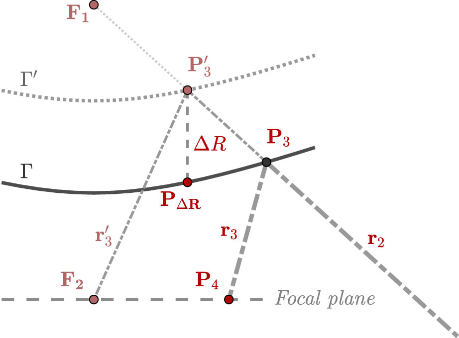
The signal path variations are derived by spatial ray tracing taking not only rotationally but also nonrotationally symmetric deformation patterns into account in this contribution. As shown in Figure 1(a), a rotationally symmetric deformation pattern represents a homologous deformation that only affects datum-independent parameters or shifts along the optical axis. For instance, a uniformly applied scaling of components belongs to this deformation pattern. Applying equation (1) considers only these deformations.

$Figure 1 Comparison of rotationally symmetric and nonrotationally symmetric deformation patterns and their impact on the ray path, which is segmented in the segment lengths D i {D}_{i} and the corresponding normalized direction vectors r i {{\bf{r}}}_{i} . Deformed components are shown in solid black lines. (a) Symmetric deformations caused by a displacement of the vertex and a vertical shift of the subreflector along the optical axis as well as a variation of the focal length of the main reflector. (b) Asymmetric deformations caused by a horizontal shift and a tilting of the subreflector.$

Figure 1

Comparison of rotationally symmetric and nonrotationally symmetric deformation patterns and their impact on the ray path, which is segmented in the segment lengths D i and the corresponding normalized direction vectors r i . Deformed components are shown in solid black lines. (a) Symmetric deformations caused by a displacement of the vertex and a vertical shift of the subreflector along the optical axis as well as a variation of the focal length of the main reflector. (b) Asymmetric deformations caused by a horizontal shift and a tilting of the subreflector.

Nonrotationally symmetric deformation patterns occur whenever the optical axis of the whole feed unit is not identical to the axis of symmetry of each single component of the feed unit and are depicted in Figure 1(b). This deformation involves, for instance, a displacement or a tilting of a single component. In either case, the form type of the components remains unchanged.

Figure 1 compares rotationally symmetric and nonrotationally symmetric deformation patterns as well as their impact on the ray path. Neuralgic points such as the focal points F 1 and F 2 , the vertex P v , and the mounting points P m of the main reflector are shown for the nondeformed case. A certain signal ray path is segmented in the segment lengths D i and the corresponding normalized direction vectors r i . The reference plane and the focal plane define the start point and the end point of the ray path, respectively.

For the sake of completeness, there is a third class of deformation pattern that unpredictably deforms the form of components such as local fabrication discrepancies of the reflector surface. Due to their unpredictable character, these deformations are not taken into account in this analysis. It is assumed that this kind of deformation is small and not affecting the SPV significantly. In particular, the panels of the main reflector are stiff designed, and their positions have been validated by the manufacturer at GOW.

The signal path variation is evaluated by numerical integration. Using appropriate step sizes, the SPV is obtained from

(2) Δ L ( ε ) = ∑ ϕ = 0 2 π ∑ r = 0 R I n ( γ ϕ , r ) r Δ D ϕ , r ( ε ) ∑ ϕ = 0 2 π ∑ r = 0 R I n ( γ ϕ , r ) r ,

where I n is the intrinsic normalized illumination function of the VLBI radio telescope, r is the distance between the axis of symmetry of the main reflector and the incoming ray, γ is the aperture angle with respect to the optical axis, and Δ D denotes the change of the path length. The inner sum corresponds to radial distances r along the ϕ th meridian. The outer sum relates to the number of pie slices covering the full circle.

To derive the SPV, the geometries of the main reflectors as well as the geometries of the subreflectors have to be parameterized. Sections 2.1 and 2.2 present the basic equations to parametrize the main reflector and the subreflector of the RTW and the TTW-2, respectively. Section 2.3 deals with the change Δ D of the ray path length introduced in equation (2).

2.1 Radio telescope Wettzell

The 20 m Radio Telescope Wettzell was constructed in the early 1980s and has been in operation since 1983 (Schüler et al. 2015). The RTW is part of the legacy VLBI network and is one of the VLBI radio telescopes with the longest history in geodetic VLBI as well as one of the most engaged station with geodetic VLBI sessions (Neidhardt et al. 2007). The RTW contributes to the IVS and partly other partners such as the European VLBI network (EVN) (Neidhardt et al. 2021).

The main reflector is parameterized by a rotationally symmetric paraboloid, having only one datum-independent form parameter a . The canonical form is given by (Lösler et al. 2017)

(3) a 2 ( x i 2 + y i 2 ) = z i ,

where vector p i T = ( x i y i z i ) contains the coordinates of an arbitrary surface point. In the canonical form, the paraboloid opens upward and the axis of symmetry is identical to the z -axis. The scale parameter a widens the opening of the paraboloid and relates to the focal length via

(4) F = 1 4 a 2 .

Introducing five additional isometric parameters, i.e., three translation parameters P 0 T = ( X 0 Y 0 Z 0 ) as well as two Euler angles ω x and ω y yield an arbitrarily orientated paraboloid in space. The common rigid transformation considering the rotational symmetry is given by

(5) p i = R x ( ω x ) R y ( ω y ) ( P i − P 0 ) ,

where R are orthogonal matrices and denote basic rotations around the subindexed axis of the (co-rotated) frame. The translation vector P 0 is identical with the three coordinate components of the vertex position P v . The surface point P i relates to the arbitrarily orientated frame of the paraboloid and corresponds to the canonical frame position p i .

The RTW is a Cassegrain type VLBI radio telescope, i.e., the subreflector is located in front of the primary focal point F 1 . The subreflector is parameterized by a rotaionally symmetric hyperboloid of two sheets. The canonical form reads (Bronshtein et al. 2007, p. 220):

(6) − x i 2 + y i 2 A 1 2 + z i 2 A 2 2 = 1 ,

where A 1 and A 2 denote the semi-axes. Substituting equation (5) into equation (6) yields an arbitrarily orientated hyperboloid in space. A point P i lying on the surface of the subreflector fulfills the following condition:

(7) ∣ ‖ F 2 P i ‖ 2 − ‖ F 1 P i ‖ 2 ∣ = 2 A 2 ,

where F 1 and F 2 are the focal points.

Figure 2 depicts a cross-sectional view of a Cassegrain type radio telescope. The incoming ray is reflected by the main reflector toward the subreflector, i.e., in the direction of the joint focal point F 1 . The second reflection occurs at the subreflector, where the ray is reflected into the system focal point F 2 of the feed unit. The incidence angle at F 2 with respect to the axis of symmetry is γ . Each ray path can be divided into three segments of length D i . In case of a nondeformed VLBI radio telescope, the sum of these segment lengths is identical for all rays. Nominal values of the RTW are summarized in Table 1.

$Figure 2 A cross-sectional view of a Cassegrain-type VLBI radio telescope with ray paths. The subreflector is implied by a hyperbola, and the main reflector is drawn as a parabola. Physical parts of both reflectors are shown in solid black lines. F 1 {{\bf{F}}}_{1} is the joint focal point of both reflectors, F 2 {{\bf{F}}}_{2} is the unique system focal point, and γ \gamma is the aperture angle of the feed unit. The vertex of the paraboloid is denoted by P v {{\bf{P}}}_{{\rm{v}}} . The distances D i {D}_{i} and the corresponding normalized direction vectors r i {{\bf{r}}}_{i} are segments of a ray path. Mounting points are indicated by P m {{\bf{P}}}_{{\rm{m}}} .$

Figure 2

A cross-sectional view of a Cassegrain-type VLBI radio telescope with ray paths. The subreflector is implied by a hyperbola, and the main reflector is drawn as a parabola. Physical parts of both reflectors are shown in solid black lines. F 1 is the joint focal point of both reflectors, F 2 is the unique system focal point, and γ is the aperture angle of the feed unit. The vertex of the paraboloid is denoted by P v . The distances D i and the corresponding normalized direction vectors r i are segments of a ray path. Mounting points are indicated by P m .

Table 1

Nominal values of the feed unit of the RTW antenna (DOMES: 14201S004)

Component	Description	Value
Main reflector	Focal length	9 m
	Radius (physical)	10 m
	Separation of mount points	4.4 m
Subreflector	Distance from vertex to system focal	2.55 m
	Radius (physical)	1.35 m
	Radius (illuminated)	1.32 m
Aperture	Maximum aperture angle	13.2 ∘

2.2 Twin telescope Wettzell

The Global Geodetic Observing System (GGOS) aims for an accuracy of 1 mm in the position on a global scale, which has not been achieved yet (Rothacher et al. 2009, Plag et al. 2010). To meet these requirements, among others, the existing VLBI network is being extended by a new generation of VLBI radio telescopes (Niell et al. 2006). These telescopes are referred to as VGOS radio telescopes. They are characterized by a more compact and stiffer construction and are designed for broadband reception. As shown in Figure 2, the subreflector of legacy VLBI radio telescopes shadows the surface of the main reflector and, hence, induces a field of decreased intensity (Cutler 1947). To increase the sensitive area of the main reflector, most of the VGOS-specified radio telescopes make use of an improved reflector design known as ring-focus paraboloid.

Since 2013, the GOW operates two VGOS-specified radio telescopes. Both VLBI radio telescopes are identical in construction and are referred to as Twin Telescopes Wettzell (TTW). The northern twin VLBI radio telescope (TTW-1) acts as a legacy S/X station, and the southern TTW-2 contributes to the VGOS network and participates in almost all VGOS and EU-VGOS sessions (Neidhardt et al. 2021). The TTW antennas make use of the improved main reflector design, and both VLBI radio telescopes are equipped with a ring-focus paraboloid.

A rotationally symmetric ring-focus paraboloid integrates a circular cylinder into a rotationally symmetric paraboloid. According to Lösler et al. (2017), the canonical form is expressed by

(8) a 2 { ( x i − r c n x , i ) 2 + ( y i − r c n y , i ) 2 } = z i .

Here, r c is the radius of the cylinder and

(9a) n x , i = x i x i 2 + y i 2 ,

(9b) n y , i = y i x i 2 + y i 2

are the components of the normalized normal vector n i T = ( n x , i n y , i 0 ) , which shifts the i th position p i to the surface of the paraboloid. The datum-independent form parameter a relates to the focal length via equation (4). Substituting equation (5) into equation (8) yields an arbitrarily orientated ring-focus paraboloid in space. For r c = 0 , equation (8) parametrizes a rotationally symmetric paraboloid. For that reason, equation (8) is applicable not only for most of the legacy VLBI radio telescopes but also for a large number of VGOS-specified radio telescopes.

The TTW antennas are Gregorian type VLBI radio telescopes, and the subreflector is located behind the primary focal points F 1 , as shown in Figure 3. The main reflector reflects the incoming ray, and the reflected ray passes through a primary focal point toward the subreflector. Due to the ring-focus design, the main reflector has an infinite number of focal points F 1 forming a focal circle or ring having radius r c . The subreflector is parameterized by an elliptic spindle torus depicted in Figure 4. This form results from a rotation of a tilted ellipse around the axis of symmetry of the main reflector.

$Figure 3 Cross-sectional view of a Gregorian type VLBI radio telescope with ring-focus paraboloid. The subreflector is implied by two tilted ellipses. The main reflector consists of two shifted parabolic arcs. Physical parts of both reflectors are shown in solid black lines. F 1 {{\bf{F}}}_{1} is a point of the joint focal ring, F 2 {{\bf{F}}}_{2} depicts the unique system focal point, and γ \gamma is the aperture angle of the feed unit. The vertex is denoted by P v {{\bf{P}}}_{{\rm{v}}} . The distances D i {D}_{i} and the corresponding normalized direction vectors r i {{\bf{r}}}_{i} are segments of a ray path. Mounting points are indicated by P m {{\bf{P}}}_{{\rm{m}}} .$

Figure 3

Cross-sectional view of a Gregorian type VLBI radio telescope with ring-focus paraboloid. The subreflector is implied by two tilted ellipses. The main reflector consists of two shifted parabolic arcs. Physical parts of both reflectors are shown in solid black lines. F 1 is a point of the joint focal ring, F 2 depicts the unique system focal point, and γ is the aperture angle of the feed unit. The vertex is denoted by P v . The distances D i and the corresponding normalized direction vectors r i are segments of a ray path. Mounting points are indicated by P m .

Figure 4

Cut open spatial wire-frame model of an elliptic spindle torus. The physical part of the torus corresponding to the subreflector of VGOS-specified radio telescopes is depicted in solid.

The first focal point F 1 lies on a circle, which is identical with the focal circle of the main reflector, and the second focal point F 2 is fixed at the axis of symmetry. This point corresponds to the system focal point and receives the ray with angle γ . Nominal values of the twin VLBI radio telescopes are summarized in Table 2.

Table 2

Nominal values of the feed unit of the TTW antennas (DOMES: 14201S043, 14201S044)

Component	Description	Value
Main reflector	Focal length	3.7 m
	Radius (physical)	6.6 m
	Radius (illuminated)	6.4 m
	Ring radius	0.74 m
	Separation of mount points	3.92 m
Subreflector	Distance from vertex to system focal	3.60296 m
	Radius (physical/illuminated)	0.74 m
Aperture	Maximum aperture angle	65 ∘

Let B 1 and B 2 be the semi-axes and θ be the tilting angle of the ellipse with respect to the axis of symmetry, and the canonical form describing the subreflector geometry reads (Lösler 2021, p. 112) as follows:

(10) ζ 1 2 B 1 2 + ζ 2 2 B 2 2 = 1 ,

where R θ = B 2 2 − B 1 2 sin θ is the radius with respect to the center of the ellipse, and

(11a) ζ 1 = z i sin θ + ( x i 2 + y i 2 − R θ ) cos θ ,

(11b) ζ 2 = z i cos θ − ( x i 2 + y i 2 − R θ ) sin θ .

Substituting equation (5) into equation (10) yields an arbitrarily orientated elliptical torus in space. A point P i lying on the surface of the subreflector fulfills the condition:

(12) ∣ ‖ F 2 P i ‖ 2 + ‖ F 1 P i ‖ 2 ∣ = 2 B 2 .

Therefore, the sum of the segment lengths D i is identical for all rays, if the VLBI radio telescope is not deformed.

2.3 Ray path segments

The total path length of a certain ray is obtained by summing up the segment lengths D i , as indicated by Figure 1. For that purpose, the segments are parameterized by spatial straight lines. The well-known parametric equation of a line through the point P i reads

(13) P ( D i ) = P i + D i r i ,

where r i is the normalized normal vector, and D i is the distance between P ( D i ) and P i .

According to Figure 1, the first segment corresponds to the distance between P 1 lying at the reference plane and P 2 at the main reflector. The normal vector of the reference plane is identical with the axis of symmetry of the main reflector and, thus, parallel to the incoming rays r 1 The distance between the reference plane and the mounting points P m of the main reflector is constant, as indicated in Figure 1(a). The first segment reads

(14a) P 2 = P 1 + D 1 r 1 .

The second segment describes the distance between the main reflector and the subreflector. The starting point P 2 of this segment is the intersection point of the incoming ray and the main reflector. The normal vector of the tangent plane at the specific position P 2 corresponds to the gradient vector to the surface of the main reflector. Applying the law of reflection using, for instance, the Householder transformation yields the direction r 2 of the reflected ray. The intersection point of the resulting straight line and the subreflector defines the end point P 3 of the second segment, i.e.,

(14b) P 3 = P 2 + D 2 r 2 .

P 3 is the starting point of the third segment, which describes the distance between the subreflector and the feed horn. As mentioned earlier, the gradient vector to the surface of the subreflector defines the tangent plane at the specific position P 3 , and the direction r 3 towards the feed horn results from the law of reflection. In case of a nondeformed VLBI radio telescope, the end point is identical with the system focal point F 2 . However, if components of the feed unit are deformed, the ray does not pass F 2 . According to Artz et al. (2014), the intersection point P 4 of the segment’s straight line and the focal plane defines the end of the ray path and reads

(14c) P 4 = P 3 + D 3 r 3 .

In Figure 1, the feed horn position indicated by the focal plane is assumed to be fixed with respect to the elevation axis. This is the case for the VLBI radio telescopes at Wettzell. However, if the feed horn is fixed to the vertex, the variation between the feed horn and the elevation axis has to be taken into account by a further segment according to equation (13).

The variation of a certain ray path is given by

(15) Δ D = ∑ i D i − D ˜ ,

where D ˜ is the total reference path length obtained from the nondeformed VLBI radio telescope. By applying equation (2), the SPV results from the evaluation of the weighted sum of these variations.

3 Illumination function

The illumination describes the exploited intensity of the areas of the aperture. This telescope-specific function is usually rotationally symmetric and introduced as a zonal weighting scheme. The illumination function reduces the influence of errors by down weighting regions of low intensity in the outer aperture area (Baars 2007, Ch. 4.2). The normalized illumination function I n is directly introduced in equation (2) to weigh the variations Δ D of the ray paths. In equation (1), the deformation components Δ R , Δ V , and Δ F are weighted by the corresponding weighting coefficients α R , α V , and α F . As shown by Clark and Thomsen (1988), these weighting coefficients are linear dependent, i.e.,

(16a) α F = λ ( 1 − α R ) ,

(16b) α V = − λ α R , if λ ′ = λ = 2 , − 1 − λ α R , otherwise .

The mounting of the feed horn of secondary focus VLBI radio telescopes affects the resulting SPV and is parametrized by λ = 2 , see equation (1). Depending on the mount, the feed horn has a fixed distance to the vertex, indicated by λ ′ = 1 , or a fixed distance to the elevation axis, indicated by λ ′ = 2 (Nothnagel et al. 2019).

As already mentioned, the mount of the feed horn is fixed with respect to the elevation axis, i.e., λ ′ = 2 , for the VLBI radio telescopes at Wettzell. Integrating the individual ray paths, which are weighted by the normalized telescope-specific illumination function I n over the entire aperture, yields (Lösler et al. 2019):

(16c) α R = ∫ γ min γ max I n ( γ ) h ( γ ) d γ .

Here, γ min and γ max denote the integration limits, and h is a function modeling the γ -dependent extra path length on the subreflector due to a vertical deformation Δ R .

The resulting extra path length caused by a displacement Δ R of the subreflector along the optical axis can be appropriately approximated by utilizing the geometric property of the subreflector. According to equation (7), for Cassegrain type VLBI radio telescopes, the extra path length results from (Lösler 2021, p. 116)

(17a) h ( γ ) = 1 2 Δ R ( ∣ ‖ P 4 P 3 ‖ 2 − ‖ F 1 P 3 ‖ 2 ∣ − 2 A 2 ) .

As shown in Figure 5, the subreflector is displaced by Δ R . The incoming ray is reflected at P 3 instead of P 3 ′ , and the ray achieves the focal plane at P 4 , see also Figure 1. The downward induced vertical displacement Δ R shortens the ray path length modeled by h . Following the same line of reasoning and in compliance with equation (12), the extra path length of Gregorian type VLBI radio telescopes is given by (Lösler et al. 2019)

(17b) h ( γ ) = 1 2 Δ R ( ∣ ‖ P 4 P 3 ‖ 2 + ‖ F 1 P 3 ‖ 2 ∣ − 2 B 2 ) .

The angle of incidence γ with respect to the optical axis can readily be obtained from the direction of the incoming ray path r 1 and the received ray path r 3 , i.e.,

(18) cos γ = r 1 T r 3 .

The factor 1 2 in equation (17) ensures the consistency with the common definition of α R derived by Abbondanza and Sarti (2010).

$Figure 5 Cross-sectional view of a part of the subreflector of a Gregorian type VLBI radio telescope. The unshifted subreflector Γ ′ \Gamma ^{\prime} is shown as a hyperbola with focal points F 1 {{\bf{F}}}_{1} and F 2 {{\bf{F}}}_{2} in dotted style. The solid hyperbola represents the subreflector Γ \Gamma shifted vertically by Δ R \Delta R . The quantities of the reference state are denoted by an apostrophe. The signal ray path is depicted for the deformed as well as the nondeformed case, where r {\bf{r}} are normalized direction vectors.$

Figure 5

Cross-sectional view of a part of the subreflector of a Gregorian type VLBI radio telescope. The unshifted subreflector Γ ′ is shown as a hyperbola with focal points F 1 and F 2 in dotted style. The solid hyperbola represents the subreflector Γ shifted vertically by Δ R . The quantities of the reference state are denoted by an apostrophe. The signal ray path is depicted for the deformed as well as the nondeformed case, where r are normalized direction vectors.

Especially for legacy VLBI radio telescopes, the illumination function is often undocumented and has to be reconstructed from discrete samples. Samples can be determined, for instance, by discrete measurements, by simulations, or by beam diagrams. Suitable functions to model the illumination are evaluated by Abbondanza and Sarti (2010). Since the best approximation of the field radiated by a circular feed horn is a Gaussian beam, the authors highly recommend a Gaussian function, see the contribution by Abbondanza and Sarti (2010) and the references inside.

Figure 6 depicts the discrete amplitude sample points of the RTW and the TTW-2, respectively. According to the recommendation given by Abbondanza and Sarti (2010), a common Gaussian function, i.e.,

(19) I ( γ ) = g 0 exp − ( γ − g 1 ) 2 g 2 2 ,

with coefficients g 0 , g 1 , and g 2 is used to derive the telescope-specific illumination functions. Here, the height and the position of the curve’s peak are parametrized by g 0 and g 1 . The width of the bell-shaped curve is controlled by g 2 (Carlton and Devore 2017, p. 172). Numerical values of the determined coefficients are summarized in Table 3, and the resulting functions are shown in red in Figure 6.

Figure 6

Estimated amplitude functions. Red dots denote the amplitude samples of the RTW (a) and the TTW-2 (b), respectively. The related Gaussian functions are depicted in red.

Table 3

Estimated coefficients of the telescope-specific illumination functions as well as the integration limits for the RTW and the TTW-2

Parameter	RTW	TTW-2
g 0	− 30.56 dB ± 6.89 dB	− 34.59 dB ± 4.60 dB
g 1	23.2 5 ∘ ± 3.2 2 ∘	125.3 9 ∘ ± 9.4 5 ∘
g 2	10.5 4 ∘ ± 1.9 7 ∘	61.6 6 ∘ ± 5.0 9 ∘
γ min	1.8 ∘	0.0 ∘
γ max	13.2 ∘	65.0 ∘

To serve as a weighting function of the full aperture, the illumination function has to be transferred to decimal units and to be normalized using the normalization factor k g . This factor results from (Abbondanza and Sarti 2010, Artz et al. 2014)

(20) 1 k g = 2 π ∫ γ min γ max 1 0 g 0 exp − ( γ − g 1 ) 2 g 2 2 10 d γ ,

where γ min and γ max denote the integration limits that correspond to the illuminated part of the aperture, see Table 3. These integration limits result from the nominal values given in Tables 1 and 2. Finally, the normalized illumination function reads

(21) I n ( γ ) = k g 1 0 g 0 exp − ( γ − g 1 ) 2 g 2 2 10 ,

and the weights of the VLBI delay model given by equation (1) are obtained from equation (16).

Table 4 summarizes the resulting weighting coefficients for both VLBI radio telescopes under investigation. The largest weights α V can be found for variations of the vertex Δ V . Therefore, even small variations Δ V contribute significantly to the SPV (Artz et al. 2014).

Table 4

Weights of the VLBI delay model for the RTW and the TTW-2

Telescope	DOMES	α V	α F	α R
RTW	14201S004	− 2.11	− 0.11	+1.05
TTW-2	14201S044	− 1.27	+0.73	+0.64

The focal length variation Δ F itself is a descriptive parameter commonly associated with gravitational deformation of VLBI radio telescopes. For legacy VLBI radio telescopes, this variation has only a minor impact on the SPV because Δ F is down-weighted by α F , see also the contribution by Bergstrand et al. (2019). However, this conclusion cannot be generalized because the effect of focal length variations can be significant for VGOS-specified radio telescopes as shown by Lösler et al. (2019).

4 Analysis and results

To measure deformations at VLBI radio telescopes, several methods have been evaluated, especially in the last decade. Holography (Nikolic et al. 2007, Hunter et al. 2011), close-range photogrammetry (Shankar et al. 2009, Lösler et al. 2019), and polar measurement systems such as laser scanners (Bleiders 2020, Salas et al. 2022) or laser trackers (Fu et al. 2015) have been successfully applied to investigate gravitational deformations of VLBI radio telescopes. For a survey of techniques, the interested reader is referred to Baars (2007, Ch. 6). Regardless of the used measurement method, the observed points as well as the related dispersion matrix are treated as incoming data to study the deformation behavior of VLBI radio telescopes.

In this contribution, data sets obtained from close-range photogrammetry using an unmanned aerial vehicle (UAV) are investigated. The data were acquired during a measurement campaign at GOW in the fall of 2021. The RTW and the TTW-2 were measured from 10° to 90° in elevation using a step-size of 10°. For the RTW, an additional experiment was performed at ε = 5°. Each data set refers to a specific elevation position and consists of observed points located at the main reflector, at the backside of the subreflector, and at construction elements such as the tube or the support struts, see Table 5. The number of glued targets depends on the dimension of the components of the receiving unit (see Tables 1 and 2), and, therefore, varies between both telescopes under investigation. Figure 7 shows the prepared TTW-2 that was equipped with discrete black and white coded targets. The UAV carrying the photogrammetric camera is visible in front of the TTW-2 main reflector.

Figure 7

Unmanned aerial vehicle in front of the prepared VGOS radio telescope TTW-2, which is equipped with photogrammetric targets at the receiving unit.

Table 5

Number of observed points at the RTW and the TTW-2

Component	RTW	TTW-2
Main reflector	169	112
Subreflector	6	10
Tube	16	36
Support struts	44	0

The observed points and the related fully populated dispersion matrix are obtained from a bundle adjustment using the in-house software package JAiCov (JAiCov 2021). During the bundle adjustment, the data sets were scaled uniformly to the reference temperature T ₀ = 7.8°C used in VLBI data analysis (Nothnagel 2008), to obtain comparable and combinable results.

The deformations of the main reflectors and the subreflectors are addressed in Sections 4.1 and 4.2. The resulting signal path variations are presented in Section 4.3. Hereafter, subscripts R and T indicate the results of the RTW and the TTW-2, respectively.

4.1 Main reflector deformations

The ten data sets acquired at the RTW as well as the nine data sets from the TTW-2 are analyzed individually. The parameters of the main reflector are adjusted by means of least-squares treating the points observed at the main reflector surface as observations. The functional model introduced for the RTW and TTW-2 is given by equations (3) and (8), respectively. The stochastic model results from the fully populated dispersion matrix of the observed surface points. Since the points were marked by glued-on targets, the thickness of the targets w = 80 μ m and the corresponding uncertainty σ w = 15 μ m have to be taken into account during the adjustment. For that purpose, the gradient vector to the surface at each point is determined and the observed position corrected for the target thickness. Since the gradient vectors are unknown beforehand, this compensation must be applied iteratively.

The estimated focal lengths F R of the RTW are depicted in Figure 8. The error bars indicate the 95% confidence interval of a single measurement value. The curvature of the main reflector decreases, the surface becomes flatter and the estimated focal length increases while the telescope rotates upwards from 0 ° to 9 0 ° . The variation of the estimated focal length is about 10 mm and is comparable to values reported for legacy VLBI radio telescopes having a similar dimension (see the contributions by Sarti et al. 2009b, Holst et al. 2017).

$Figure 8 Estimated focal lengths F R {F}_{{\rm{R}}} and corresponding prediction function of the RTW. The error bars and the error band indicate the 95% confidence interval of a single measured value (red dots) and the prediction function (black line), respectively.$

Figure 8

Estimated focal lengths F R and corresponding prediction function of the RTW. The error bars and the error band indicate the 95% confidence interval of a single measured value (red dots) and the prediction function (black line), respectively.

These discrete focal lengths are adapted by a common sine function given by

(22) F R ( ε ) = 8.9890 m + 11.83 mm ⋅ sin ( 0.641 ε ) ,

which is depicted in black together with the related 95% confidence interval in Figure 8. The standard deviations of the coefficients, i.e., the shift, the amplitude, and the damping factor, are 0.9 mm, 4.6 mm, and 0.37, respectively.

For ε = 9 0 ° , the focal length is F R ( 9 0 ° ) = 8.9990 m . Assuming that the nominal values given in Table 1 are referred to 20 ° C commonly used in mechanical engineering, the adapted nominal focal length is F ˜ R ( 7.8 ° C ) = 8.9987 m and deviates only by about 0.3 mm. Moreover, Dutescu et al. (1999) applied a terrestrial laser scanner at the RTW to derive the focal length of the main reflector, and reported a deviation from the nominal focal length of about 13 mm at the lowest elevation position. This value is confirmed in this investigation, see Figure 8.

Figure 9 depicts the estimated focal lengths F T of the TTW-2 as well as the related 95% confidence intervals. The estimate deviates clearly at ε = 5 0 ° . Due to the tilt of the camera mounted at the UAV, it is more challenging to take images of the main reflector surface than, for instance, in a configuration close to the nadir, because the orientation of the UAV has to be taken into account (Greiwe et al. 2020). Due to this discrepancy, the data set at 50 ° is excluded from further analyses, and is depicted in gray.

$Figure 9 Estimated focal lengths F T {F}_{{\rm{T}}} and corresponding prediction function of the TTW-2. The error bars and the error band indicate the 95% confidence interval of a single measured value (blue dots) and the prediction function (black line), respectively. The grayed out value at 50 ° {50}^{^\circ } is shown for completeness, but it is not used within the analysis.$

Figure 9

Estimated focal lengths F T and corresponding prediction function of the TTW-2. The error bars and the error band indicate the 95% confidence interval of a single measured value (blue dots) and the prediction function (black line), respectively. The grayed out value at 50 ° is shown for completeness, but it is not used within the analysis.

An adapted cosine function is applied to predict the focal length variations of the TTW-2. The determined prediction function reads

(23) F T ( ε ) = 3.6998 m − 1.07 mm ⋅ cos ε

and is depicted in black together with the related 95% confidence interval in Figure 9. The standard deviations of the coefficients, i.e., the shift and the amplitude, are 0.3 mm and 0.4 mm, respectively.

Similar to the RTW, the focal length increases with the increasing elevation. However, the maximum variation of about 1 mm is considerably smaller than for the RTW, but is comparable to the value reported for a VGOS-specified radio telescope at the Onsala Space Observatory (Lösler et al. 2019). The estimated focal length at ε = 9 0 ° is F T ( 9 0 ° ) = 3.6998 m and differs from the nominal value F ˜ T ( 7.8 ° C ) = 3.6995 m by about 0.3 mm.

As indicated in Figure 1(a), the vertex position Δ V is affected by a change Δ F in the focal length due to the position of the main reflector mount P m (Nothnagel et al. 2019). In virtue of equations (3), (8), and (4), the resulting shift can readily be expressed by

(24) Δ V ( ε ) = ( s m − r c ) 2 4 1 F ( 9 0 ° ) − 1 F ( ε ) ,

where F ( 9 0 ° ) is the reference focal length, r c is the ring radius, and s m is the radial distance from the mount to the axis of symmetry of the main reflector, which is known from the structural design of the telescope construction. For the RTW, the radial distance is s m = 4.4 m 2 and the ring radius is omitted by r c = 0 , see Table 1. For the TTW-2, the radial distance is s m = 3.92 m 2 and the ring radius is r c = 0.74 m , see Table 2. The maximum shift Δ V ( 0 ° ) of the RTW and the TTW-2 is − 0.3 mm and − 0.1 mm , respectively. These values are quite small but are scaled by α V within the VLBI delay model, which are by far the largest weights, as shown in Table 4.

4.2 Subreflector variations

The variations of the subreflector are investigated using the positions of targets glued on the backside of the subreflector, see Table 5. The subreflector itself is assumed to be stiff and untwisted due to its small size compared to the main reflector.

The mounting of the subreflector differs for both telescopes. Although the quadrupod of the RTW holding the subreflector is fixed in construction, the subreflector of the TTW-2 is equipped with a so-called hexapod. The hexapod mechanically compensates for defocused optics caused by gravitational deformations by spatially shifting and rotating the subreflector (Schüler et al. 2015). In geodetic VLBI, the subreflector is kept fixed, and the hexapod of the TTW-2 is set to inactive. To verify the consistency of the mechanical compensation with respect to the VLBI delay model, the TTW-2 was observed with active hexapod and with fixed hecapod.

4.2.1 RTW subreflector variations

Beside the focal length F , isometric parameters describing the position and the orientation of the main reflector are estimated. The position is defined by the vertex P v and the orientation corresponds to r 1 . These parameters define the axis of symmetry by a spatial straight line, defined by equation (13). To obtain the variations of the subreflector Δ R along the axis of symmetry, the positions of the six targets mounted at the backside of the subreflector are orthogonally projected onto this axis. The variations of the relative distances between the vertex and the projected positions indicate the subreflector variations and are shown in Figure 10.

$Figure 10 Estimated distances between the vertex of the main reflector and the projected position of the mounted targets at the subreflector with respect to 90 ° {90}^{^\circ } . Error bars indicate 95% confidences.$

Figure 10

Estimated distances between the vertex of the main reflector and the projected position of the mounted targets at the subreflector with respect to 90 ° . Error bars indicate 95% confidences.

The variations clearly depend not only on the elevation angle but also on the target position. Almost identical values can be found for the points 459 and 460, for the points 427 and 455, as well as for the points 428 and 454. Moreover, the variations of the points 428 and 454 are negative but almost identical in magnitude to those of the points 427 and 455.

Figure 11 shows the configuration of the six targets at the backside of the subreflector. The points 427, 428, 454, and 455 are symmetrically distributed with respect to the horizontal central axis. Although positive variations are obtained for the points that are located below this axis, negative values result from the points located above this axis. For that reason, the variations depicted in Figure 10 result from a small shift overlaid by an additional tilt of the subreflector. Moreover, the horizontal central axis is close to the tiling axis.

$Figure 11 Target positions at the backside of the subreflector of the RTW. The center of the subreflector is indicated by P c {{\bf{P}}}_{{\rm{c}}} .$

Figure 11

Target positions at the backside of the subreflector of the RTW. The center of the subreflector is indicated by P c .

The center of the subreflector P c can easily be reconstructed from the image data and is (almost) unaffected by a subreflector tilt. The shift values of the subreflector Δ R depicted in Figure 12 are obtained from the relative distances between the projected position of P c onto the axis of symmetry and the vertex position P v of the main reflector. The error bars indicate the 95% confidence interval of a single measurement value. The maximum shift of the subreflector is about 1 mm and, thus, 10 times smaller compared to the maximum focal length variation. In contrast to the focal length variations depicted in Figure 8, which decrease, while the curvature of the main reflector increases, the subreflector shifts along the optical axis in the opposite direction. The estimated distances between the subreflector and the vertex decrease, while the telescope rotates from 0 ° to 9 0 ° . The adapted prediction function reads

(25) Δ R R ( ε ) = 0.96 mm ⋅ ( 1 − sin ε )

and is depicted in black together with the related 95% confidence interval. The estimated standard deviation of the amplitude is 0.2 mm.

$Figure 12 Estimated shift values Δ R R \Delta {R}_{{\rm{R}}} of the subreflector and corresponding prediction function of the RTW. The error bars and the error band indicate the 95% confidence interval of a single measured value (red dots) and the prediction function (black line), respectively.$

Figure 12

Estimated shift values Δ R R of the subreflector and corresponding prediction function of the RTW. The error bars and the error band indicate the 95% confidence interval of a single measured value (red dots) and the prediction function (black line), respectively.

A tilt of the subreflector describes the vertical angular deviation between the symmetry axes of the subreflector and the main reflector. It belongs to the class of nonrotationally symmetric deformation patterns. For the Medicina VLBI radio telescope, a tilt of the quadrupod holding the subreflector was reported by Sarti et al. (2009a). However, the tilt was not considered within the VLBI delay model by the authors.

Assuming an untwisted subreflector, the normal vector of the plane defined by the six targets at the backside is an appropriate approximation of the axis of symmetry of the subreflector to investigate the relative tilt of the subreflector. Figure 13 depicts the derived angular deviations Δ τ R with respect to 90 ° . Error bars indicate the related 95% confidences. From these measured values, a cosine function is adapted to predict the tilt of the subreflector with respect to the axis of symmetry of the main reflector. The prediction function reads

(26) Δ τ R ( ε ) = − 0.2 9 ° ⋅ cos ε

and is depicted in black together with the related 95% confidence interval. The estimated standard deviation of the amplitude is 0.02 ° . The maximum tilt in magnitude is about Δ τ R ( 0 ° ) = − 0 . 3 ° and leads to a nonrotationally symmetric signal path variation as indicated in Figure 1(b).

$Figure 13 Estimated tilts Δ τ R \Delta {\tau }_{{\rm{R}}} of the subreflector and corresponding prediction function of the RTW. The error bars and the error band indicate the 95% confidence interval of a single measured value (red dots) and the prediction function (black line), respectively.$

Figure 13

Estimated tilts Δ τ R of the subreflector and corresponding prediction function of the RTW. The error bars and the error band indicate the 95% confidence interval of a single measured value (red dots) and the prediction function (black line), respectively.

Another nonrotationally symmetric deformation pattern results from a shift Δ S of the subreflector perpendicular to the optical axis. To investigate this deformation behavior, the vertical distances from P c to the optical axis are derived. The shift values and the adapted prediction function, i.e.,

(27) Δ S R ( ε ) = 3.25 mm ⋅ ( 1 − sin ε ) ,

are shown in Figure 14. The estimated standard deviation of the amplitude is 3.4 mm.

$Figure 14 Estimated shift values Δ S R \Delta {S}_{{\rm{R}}} of the subreflector and corresponding prediction function of the RTW. The error bars and the error band indicate the 95% confidence interval of a single measured value (red dots) and the prediction function (black line), respectively.$

Figure 14

Estimated shift values Δ S R of the subreflector and corresponding prediction function of the RTW. The error bars and the error band indicate the 95% confidence interval of a single measured value (red dots) and the prediction function (black line), respectively.

The displacement Δ S R of the subreflector varies in a range of about 3 mm and, thus, is three times larger than the estimated shift along the optical axis Δ R R shown in Figure 12. Moreover, the subreflector shifts upwards with respect to the optical axis while the telescope rotates downwards from 9 0 ° to 0 ° . The uncertainties are quite large because smallest deviations in the estimated axis of symmetry bias the results. For that reason, further investigations are recommended to verify this deformation behavior.

4.2.2 TTW-2 subreflector variations

The TTW-2 is equipped with a movable hexapod holding the subreflector to mechanically compensate for gravity-induced deformations. For that reason, the variations of the subreflector are investigated for the case of a fixed subreflector as well as for the case of an active subreflector. Hereafter, superscripts f and a indicate the configuration with fixed and active subreflector, respectively.

Similar to the RTW, the variations are obtained from mounted targets at the backside of the subreflector. These targets are symmetrically distributed at the subreflector. A best-fit plane is adjusted, and the intersection point of the plane and the axis of symmetry of the main reflector is determined. The variation Δ R along the optical axis is obtained from the distance between the intersection point and the vertex position.

Figure 15 depicts the estimated shift values Δ R T and the related 95% confidence intervals for both configurations under consideration. The adapted prediction functions read

(28a) Δ R T f = 1.16 mm ⋅ ( 1 − sin ε ) ,

(28b) Δ R T a = − 0.41 mm ⋅ ( 1 − sin ε ) ,

and are shown in black. Here, Δ R T f corresponds to the measurement configuration with a fixed subreflector shown in Figure 15(a), and Δ R T a depicted in Figure 15(b) is the prediction function of the configuration with an active subreflector. The standard deviation of the estimated amplitudes is almost identical and reads 0.7 mm. Similar to the RTW, the shift of the fixed subreflector along the optical axis is opposite with respect to the focal length variations. If the hexapod is active and compensates for gravitational inducted deformations, the shift of the subreflector along the optical axis is clearly reduced. The maximum value is reduced from 1.2 to − 0.4 mm .

$Figure 15 Estimated shift values Δ R T \Delta {R}_{{\rm{T}}} of the subreflector and corresponding prediction function of the TTW-2 for (a) a fixed subreflector and (b) an active subreflector. The error bars and the error band indicate the 95% confidence interval of a single measured value (blue and orange dots) and the prediction function (black line), respectively. The grayed out values at 50 ° {50}^{^\circ } are shown for completeness, but are not used within the analysis.$

Figure 15

Estimated shift values Δ R T of the subreflector and corresponding prediction function of the TTW-2 for (a) a fixed subreflector and (b) an active subreflector. The error bars and the error band indicate the 95% confidence interval of a single measured value (blue and orange dots) and the prediction function (black line), respectively. The grayed out values at 50 ° are shown for completeness, but are not used within the analysis.

The normal vector of the estimated plane is an appropriate approximation of the axis of symmetry of the subreflector and indicates the relative tilt of the subreflector with respect to the axis of symmetry. The angular derivations Δ τ T are determined for the case of a fixed subreflector as well as for the case of an active subreflector, and depicted in Figure 16. The deformation behavior of the fixed subreflector of the TTW-2 is similar to the RTW, see Figure 13. The prediction functions given by

(29a) Δ τ T f = − 0.0 2 ° ⋅ cos ε ,

(29b) Δ τ T a = 0.0 1 ° ⋅ cos ε

are depicted in black together with the related 95% confidence interval. The standard deviation of the estimated amplitudes is almost identical and reads 0.07 ° .

$Figure 16 Estimated tilts Δ τ T \Delta {\tau }_{{\rm{T}}} of the subreflector and corresponding prediction function of the TTW-2 for (a) a fixed subreflector and (b) an active subreflector. The error bars and the error band indicate the 95% confidence interval of a single measured value (blue and orange dots) and the prediction function (black line), respectively. The grayed out values at 50 ° {50}^{^\circ } are shown for completeness, but are not used within the analysis.$

Figure 16

Estimated tilts Δ τ T of the subreflector and corresponding prediction function of the TTW-2 for (a) a fixed subreflector and (b) an active subreflector. The error bars and the error band indicate the 95% confidence interval of a single measured value (blue and orange dots) and the prediction function (black line), respectively. The grayed out values at 50 ° are shown for completeness, but are not used within the analysis.

In case of a fixed subreflector, the amplitude is only about − 0.02 ° . Compared to the maximum tilt of the subreflector of the RTW, this value is more than 10 times smaller. If the hexapod actively compensates for the deformation, the amplitude is reduced to 0.01 ° .

The tilt of the subreflector belongs to the class of nonrotationally symmetric deformation patterns. Due to the small angles and the short distance between the subreflector and the system focal point F 2 , the tilt has only a minor contribution to the total SPV.

A further nonrotationally symmetry deformation pattern is the displacement Δ S of the subreflector perpendicular to the optical axis, see Figure 1(b). The displacement can readily be obtained from the vertical shift between the geometric centroid of the subreflector plane and the axis of symmetry of the main reflector. The estimated shift values as well as the adapted prediction functions given by

(30a) Δ S T f = − 2.21 mm ⋅ cos ε ,

(30b) Δ S T a = 0.94 mm ⋅ cos ε ,

are depicted in Figure 17. The standard deviation of the estimated amplitudes reads 0.7 mm. The dependency between Δ S T and the elevation position is clearly visible. The magnitude of the shift Δ S T perpendicular to the symmetry axis of the main reflector is larger by a factor of about two than the shift Δ R T along this symmetry axis. The maximum value is − 2 mm and 1 mm for the configuration using a fixed subreflector and an active subreflector, respectively. In contrast to the results obtained from the RTW, the fixed subreflector of the TTW-2 shifts downwards with respect to the optical axis, while the telescope rotates downwards from 9 0 ° to 0 ° .

$Figure 17 Estimated shift values Δ S T \Delta {S}_{{\rm{T}}} of the subreflector and corresponding prediction function of the TTW-2 for (a) a fixed subreflector and (b) an active subreflector. The error bars and the error band indicate the 95% confidence interval of a single measured value (blue and orange dots) and the prediction function (black line), respectively. The grayed out values at 50 ° {50}^{^\circ } are shown for completeness, but are not used within the analysis.$

Figure 17

Estimated shift values Δ S T of the subreflector and corresponding prediction function of the TTW-2 for (a) a fixed subreflector and (b) an active subreflector. The error bars and the error band indicate the 95% confidence interval of a single measured value (blue and orange dots) and the prediction function (black line), respectively. The grayed out values at 50 ° are shown for completeness, but are not used within the analysis.

4.2.3 Verification of TTW-2 subreflector variations

The detected variations Δ R , Δ τ , and Δ S are reduced, if the hexapod actively compensates for gravitationally induced deformations. However, by comparing the measured values of the configuration with a fixed subreflector and an active subreflector in Figures 15–17, an overcompensation is discernible. The introduced corrections are larger than the gravitationally induced deformations. The magnitude of the deviations is reduced, but the sign of the remaining deviations has changed.

These obtained variations strongly depend on the reliability of the derived axis of symmetry of the main reflector. In this investigation, the axis results from the adjustment of the main reflector, and is the best approximation of the true optical axis from the available data. The realized optical axis can be different from the reference axis used by the manufacturer and explains the overcompensation. For instance, the reference axis can also be defined by other construction elements of the feed unit like the tube axis, and, thus, may differ from the estimated axis of symmetry of the main reflector.

Independently of the reference axis used, the differences between the measured values of both configurations can be compared to the induced correction values of the manufacturer. The applied correction functions are industrial secret, but the resulting function values are available from the control panel of the TTW-2.

Figure 18 depicts the estimated variations obtained from the differences between the configuration with active and fixed subreflector by green dots. These differences are unaffected by gravitational deformations and describe the changes in position and orientation of the subreflector induced by the manufacturer. The related 95% confidence intervals result from the propagation of uncertainty. The applied correction values of the manufacturer with respect to 90 ° are indicated by the black dash-dotted curves. The induced correction values of the manufacturer coincide with the estimated values very well. This independent verification highlights the suitability of UAV for detecting smallest deformations not only at the feed unit of VLBI radio telescopes.

$Figure 18 Verification of the estimated variations (green dots) of the subreflector of the TTW-2 with respect to the correction values applied by the manufacturer (black dash-dotted line). (a) Verification of the shift values Δ R \Delta R along the optical axis. (b) Verification of the shift values Δ S \Delta S perpendicular to the optical axis. (c) Verification of the tilt Δ τ \Delta \tau with respect to the optical axis. The error bars indicate the 95% confidence interval of an estimate.$

Figure 18

Verification of the estimated variations (green dots) of the subreflector of the TTW-2 with respect to the correction values applied by the manufacturer (black dash-dotted line). (a) Verification of the shift values Δ R along the optical axis. (b) Verification of the shift values Δ S perpendicular to the optical axis. (c) Verification of the tilt Δ τ with respect to the optical axis. The error bars indicate the 95% confidence interval of an estimate.

4.3 Signal path variations

The aim of this investigation is to derive the signal path variations of a legacy VLBI radio telescope and a VGOS-specified radio telescope and to study the effect of nonrotationally symmetric deformation patterns. The common VLBI delay model derived by Clark and Thomsen (1988) parametrizes the SPV by a linear substitute function and considers only rotationally symmetric acting deformations. For that reason, we resort to the spatial ray tracing approach, which allows a rigorous combination of any kind of modelable deformation behavior.

According to equation (2), the SPV is evaluated by numerical integration, where Δ D takes the focal length variation Δ F , the shift of the vertex position Δ V , the displacements Δ R and Δ S of the subreflector along as well as perpendicular to the optical axis, respectively, and the tilt Δ τ of the subreflector into account. The changes Δ D of individual signal path lengths are determined for discrete positions. These positions result from 100 equidistantly distributed meridians over the entire area of the main reflector. Each meridian is sampled by 80 equidistantly distributed distances. Due to shadowing and deformations, some of the rays do not reach the main reflector or the subreflector. These rays are excluded from the analysis. Moreover, all values are referred to elevation 90 ° because we are only interested in the signal path variations. In this position, VLBI radio telescopes are assumed to be unaffected by gravity deformations.

The determined prediction functions and also the spatial ray tracing itself are nonlinear problems. Applying a linearized substitute problem to the nonlinear problem biases the estimates, because the statistical properties of linear models cannot be passed to the nonlinear case as shown by Lösler et al. (2021). The Monte-Carlo simulation is known to be an asymptotically unbiased estimator as the sample size m gets large (Rubinstein and Kroese 2017, p. 108). For that reason, a Monte-Carlo simulation is performed to estimate the SPV, using m = 50,000 samples per elevation position. In each simulation step, ray tracing is applied to a randomly deformed receiving unit. For that purpose, the components of the receiving unit are deformed using the derived predicting functions, and are overlaid by additional noise with respect to the dispersion of the predicting function coefficients.

Applying spatial ray tracing yields the red colored signal path variations of the RTW depicted in Figure 19. The light red colored error band indicates the 95% confidence interval. For comparison, the result of the VLBI delay model given by equation (1) is presented in dash-dotted style and light gray colored error band.

$Figure 19 Estimated signal path variations Δ L R \Delta {L}_{{\rm{R}}} of the RTW obtained from spatial ray tracing using equation (2) (red line with dots) and the common VLBI delay model given by equation (1) (black dash-dotted line). The corresponding 95% confidence interval is indicated by an error band in light red and in light gray, respectively. The estimates result from a Monte-Carlo simulation.$

Figure 19

Estimated signal path variations Δ L R of the RTW obtained from spatial ray tracing using equation (2) (red line with dots) and the common VLBI delay model given by equation (1) (black dash-dotted line). The corresponding 95% confidence interval is indicated by an error band in light red and in light gray, respectively. The estimates result from a Monte-Carlo simulation.

The tilt of the subreflector and the displacement of the subreflector perpendicular to the optical axis have only a minor impact onto the SPV, because both approaches yield comparable results, and the deviations are less than 0.2 mm. The maximum signal path variation is about 3.5 mm and corresponds to a time delay of about 12 ps. The maximum standard deviation is about 0.6 mm.

The signal path variations of the TTW-2 are determined for both the configuration with a fixed subreflector and the configuration with an active subreflector and are shown in Figure 20. Figure 20(a) depicts the results of the estimated SPV for the configuration with a fixed subreflector as used in regular geodetic VLBI. The result of the spatial ray tracing is given by a blue line with dots. The corresponding light blue error band indicates the 95% confidence interval. The results of the VLBI delay model are depicted by a black dash-dotted curve. The corresponding 95% confidence interval is given by the light gray colored error band. The difference between the results is less than 0.2 mm, and both approaches yield almost comparable results. Thus, the SPV is less affected by a tilt of the subreflector or a displacement of the subreflector perpendicular to the optical axis. The range of the signal path variations is about 0.9 mm and corresponds to a time delay of about 3 ps. The maximum standard deviation is 0.7 mm.

$Figure 20 Estimated signal path variations Δ L T \Delta {L}_{{\rm{T}}} of the TTW-2 obtained from spatial ray tracing using equation (2) and the common VLBI delay model given by equation (1) (black dash-dotted line); the blue line with dots corresponds to the configuration with fixed subreflector (a), and the orange line with dots corresponds to the configuration with active subreflector (b). Error bands depicted in corresponding colors indicate the 95% confidence intervals. All estimates result from Monte-Carlo simulations.$

Figure 20

Estimated signal path variations Δ L T of the TTW-2 obtained from spatial ray tracing using equation (2) and the common VLBI delay model given by equation (1) (black dash-dotted line); the blue line with dots corresponds to the configuration with fixed subreflector (a), and the orange line with dots corresponds to the configuration with active subreflector (b). Error bands depicted in corresponding colors indicate the 95% confidence intervals. All estimates result from Monte-Carlo simulations.

The resulting SPV of the TTW-2 for the configuration with active subreflector is shown in Figure 20(b). The result of the spatial ray tracing is shown in orange. The black dash-dotted curve depicts the SPV of the VLBI delay model. Error bands indicate the related 95% confidence intervals. The maximum standard deviation is 0.7 mm.

The differences between the SPV obtained from the spatial ray tracing and the SPV derived from the VLBI delay model are quite small. Both approaches yield almost comparable results. The tilt of the subreflector and the displacement of the subreflector perpendicular to the optical axis have only a minor impact onto the SPV. Therefore, the commonly used VLBI delay model is a suitable first-order delay model for legacy VLBI radio telescopes as well as for VGOS-specified radio telescopes and reduces the impact of the main gravitational-related error sources.

The maximum signal path variation of the active subreflector configuration is about − 1.4 mm and, thus, is larger in magnitude as for the configuration with fixed subreflector. The active hexapod mainly compensates for gravitationally induced deformations of the subreflector. Further deformation patterns such as the displacement of the vertex position are not considered. Therefore, the active subreflector is a subcomponent optimization. Overlaying deformation patterns can lead not only to amplification but also to attenuation and are not addressed by subcomponent optimizations. In contrast to a subcomponent optimization, the VLBI delay model and the spatial ray tracing take the interdependencies of overlaying deformations into account. For that reason, the manufacturer-specific compensation is not consistent with the VLBI delay model. Although the VLBI delay model and the spatial ray tracing compensate the elevation depended time delay of the signal, the correction introduced by the manufacturer is designed to optimize the signal strength. Both approaches compensate gravitationally inducted deformations but are incompatible.

Varenius et al. (2021) studied the impact of signal path variations onto the station coordinates of the legacy 20 m VLBI radio telescope and the 13.2 m VGOS-specified twin radio telescopes at the Onsala Space Observatory. Although the horizontal components of the station coordinates are almost unaffected, the changes in the vertical component coincide with the obtained signal-path variations. According to this finding, the difference of about 0.2 mm between the SPV obtained from spatial ray tracing and the SPV derived from the VLBI delay model affects the vertical component of the station coordinate within the same order of magnitude.

5 Conclusion

The deformation behavior of the feed unit of radio telescopes used for VLBI affects the signal path length and limits the achievable accuracy in VLBI products. Apart from fabrication discrepancies or meteorological effects, gravitationally induced deformations are identified as a crucial error source that systematically distorts the estimated vertical position of VLBI radio telescopes and, hence, biases the scale of the derived global geodetic reference frame (Altamimi et al. 2016). For that reason, working groups such as the IAG/IERS Working Group on Site Survey and Co-location (Bergstrand 2018) or joint research projects like the international GeoMetre (Pollinger et al. 2022b) project have been encouraged to investigate on gravitational deformations of VLBI radio telescopes to compensate for the systematic errors. Investigations on the deformations caused by gravity performed at several VLBI radio telescopes imply an individual VLBI radio telescope-dependent deformation behavior (see the contributions by Sarti et al. 2009a, Artz et al. 2014, Nothnagel et al. 2019). For that reason, each VLBI radio telescope or at least each type of VLBI radio telescope has to be investigated individually (Lösler et al. 2019).

The data sets used in this investigation were obtained during a measurement campaign in the fall of 2021. Mounted targets at the main reflector surface and the backside of the subreflector of the legacy 20 m VLBI Radio Telescope Wettzell as well as the southern 13.2 m Twin Telescope Wettzell were measured in several elevation positions by means of close-range photogrammetry using an unmanned aerial vehicle. Each data set consisting of the target positions and the related fully populated dispersion matrix was treated as incoming data to determine the elevation dependent path lengths.

The aim of this contribution was to study the SPV of the legacy 20 m VLBI Radio Telescope Wettzell as well as the southern 13.2 m Twin Telescope Wettzell. For the first time, the impact of nonrotationally symmetric deformation patterns onto the signal path variations were investigated. For that purpose, a spatial ray tracing procedure was introduced because the commonly used linear VLBI delay model considers only rotationally symmetric deformations. Spatial ray tracing is strongly recommended, whenever the rotationally symmetric assumption is unfounded (Lösler et al. 2018). The focal length variation Δ F , the displacement of the vertex Δ V , and the shift of the subreflector Δ R along the optical axis belong to the class of rotationally symmetric deformation patterns. Apart from that, the effect of nonrotationally symmetric deformation patterns such as the tilt of the subreflector Δ τ and the displacement Δ S of the subreflector perpendicular to the optical axis were considered for the first time.

The maximum signal path variation of the RTW obtained from spatial ray tracing is about 3.5 mm and corresponds to a time delay of about 12 ps. Although the RTW is equipped with a fixed quadrupod holding the subreflector, the TTW-2 has a movable hexapod that allows for a mechanical compensation of gravitationally induced deformations. To validate the compatibility of the mechanical compensation with the VLBI delay model, the TTW-2 was measured in two configurations. In the first configuration, the subreflector was kept fixed as it is used in regular geodetic VLBI. In the second configuration, the hexapod actively compensated for deformations caused by gravity and the subreflector was moved with respect to the elevation position of the TTW-2. Due to the compact and stiffer design of VGOS-specified radio telescopes, the SPV of these telescopes are less affected by gravitationally induced deformations. For the configuration with fixed subreflector, the range of the signal path variation is about 0.9 mm and corresponds to a time delay of about 3 ps. However, the maximum signal path variation increases, if the hexapod actively compensates for deformations. Although the active hexapod mainly compensates for gravitationally induced deformations of the subreflector, the intent of the VLBI delay model as well as the spatial ray tracing is to model the total SPV of the feed unit taking interdependencies of overlaying deformations into account. For that reason, both approaches have different intents and are incompatible.

The SPV obtained from spatial ray tracing was opposed to the results derived from the VLBI delay model. Both approaches yield almost comparable results. For that reason, the tilt of the subreflector and the displacement of the subreflector perpendicular to the optical axis have only a minor impact onto the SPV. The commonly used VLBI delay model is a suitable first-order delay model for legacy VLBI radio telescopes as well as for VGOS-specified radio telescopes and reduces the impact of the main gravitational related error sources.

# Dedicated to Prof. Dr.-Ing. Dr. H.C. Harald Schuh.

Funding information: This project 18SIB01 GeoMetre (2020) has received funding from the EMPIR programme co-financed by the Participating States and from the European Union’s Horizon 2020 research and innovation programme.
Conflict of interest: The authors declare no conflict of interest.
Data availability statement: The data sets analyzed during the current study are available from the repository at https://doi.org/10.5281/zenodo.7110033.

References

Abbondanza, Z. and X. Sarti. 2010. “Effects of illumination functions on the computation of gravity-dependent signal path variation models in primary focus and Cassegrainian VLBI telescopes.” Journal of Geodesy 84(8), 515–25, https://doi.org/10.1007/s00190-010-0389-z. Search in Google Scholar

Altamimi, Z., X. Collilieux, J. Legrand, B. Garayt, and C. Boucher. 2007. “ITRF2005: A new release of the international terrestrial reference frame based on time series of station positions and Earth orientation parameters.” Journal of Geophysical Research 112(B09401), 1–19, https://doi.org/10.1029/2007jb004949. Search in Google Scholar

Altamimi, Z., P. Rebischung, L. Métivier, and X. Collilieux. 2016. “ITRF2014: A new release of the International Terrestrial Reference Frame modeling nonlinear station motions.” Journal of Geophysical Research: Solid Earth 121(8), 6109–31, https://doi.org/10.1002/2016jb013098. Search in Google Scholar

Artz, T., A. Springer, and A. Nothnagel. 2014. “A complete VLBI delay model for deforming radio telescopes: the Effelsberg case.” Journal of Geodesy 88(12), 1145–61, https://doi.org/10.1007/s00190-014-0749-1. Search in Google Scholar

Baars, J. W. M. 2007. “The paraboloidal reflector antenna in radio astronomy and communication - theory and practice.” Number 348 in Astrophysics and Space Science Library. New York: Springer, https://doi.org/10.1007/978-0-387-69734-5. Search in Google Scholar

Bergstrand, S. 2018. “Working group on site survey and co-location.” In: IERS Annual Report 2017, edited by W. R. Dick and D. Thaller, International Earth Rotation and Reference Systems Service (IERS), Frankfurt am Main, pp. 160–1. Search in Google Scholar

Bergstrand, S., M. Herbertsson, C. Rieck, J. Spetz, C.-G. Svantesson, and R. Haas. 2019. “A gravitational telescope deformation model for geodetic VLBI.” Journal of Geodesy 93(5), 669–80, https://doi.org/10.1007/s00190-018-1188-1. Search in Google Scholar

Bleiders, M. 2020. “Electromagnetic model of dual reflector radio telescope based on laser scanning survey.” In: 2020 IEEE Microwave Theory and Techniques in Wireless Communications (MTTW), pp. 217–21, vol. 1, Riga, Latvia: IEEE. https://doi.org/10.1109/mttw51045.2020.9245071. Search in Google Scholar

Bronshtein, I. N., K. A. Semendyayev, G. Musiol, and H. Muehlig. 2007. Handbook of mathematics. 5th ed. Berlin, Heidelberg: Springer. https://doi.org/10.1007/978-3-540-72122-2. Search in Google Scholar

Carlton, M. A. and J. L. Devore. 2017. Probability with Applications in Engineering, Science, and Technology. 2nd ed, Cham: Springer. https://doi.org/10.1007/978-3-319-52401-6. Search in Google Scholar

Clark, T. A. and P. Thomsen. 1988. Deformations in VLBI Antennas. Techreport NASA-TM-100696, NASA, NASA Goddard Space Flight Center, Greenbelt, MD, United States. Search in Google Scholar

Cutler, C. C. 1947. “Parabolic-Antenna design for microwaves.” Proceedings of the IRE 35(11), 1284–94. https://doi.org/10.1109/jrproc.1947.233571. Search in Google Scholar

Dutescu, E., O. Heunecke, and K. Krack. 1999. “Formbestimmung bei Radioteleskopen mittels Terrestrischem Laserscanning.” avn 106(6), 239–45. Search in Google Scholar

Fu, L., G. Liu, C. Jin, F. Yan, T. An, and Z. Shen. 2015. “Surface accuracy analysis of single panels for the Shanghai 65-M radio telescope.” WSEAS - Transactions on Applied and Theoretical Mechanics 10(6), 54–61. Search in Google Scholar

GeoMetre. 2020. Large-Scale Dimensional Measurements for Geodesy - A Joint Research Project within the European Metrology Research Programme EMPIR, Grant Number: 18SIB01. https://doi.org/10.13039/100014132. Search in Google Scholar

Greiwe, A., R. Brechtken, M. Lösler, C. Eschelbach, and R. Haas. 2020. “Erfassung der Hauptreflektordeformation eines Radioteleskops durch UAV-gestützte Nahbereichsphotogrammetrie.” In: 40. Wissenschaftlich-Technische Jahrestagung der DGPF, vol. 29 of Wissenschaftlich-Technische Jahrestagung der DGPF, edited by T. P. Kersten, Deutsche Gesellschaft Photogrammetrie, Fernerkundung und Geoinformation e.V. pp. 346–57. Search in Google Scholar

Holst, C., D. Schunck, A. Nothnagel, R. Haas, L. Wennerbäck, H. Olofsson, R. Hammargren, and H. Kuhlmann. 2017. “Terrestrial laser scanner two-face measurements for analyzing the elevation-dependent deformation of the onsala space observatory 20-m radio telescopeas main reflector in a bundle adjustment.” Sensors 17(8, 1833), 1–21. https://doi.org/10.3390/s17081833. Search in Google Scholar PubMed PubMed Central

T. R. Hunter, F. R. Schwab, S. D. White, J. M. Ford, F. D. Ghigo, R. J. Maddalena, B. S. Mason, J. D. Nelson, R. M. Prestage, J. Ray, P. Ries, R. Simon, S. Srikanth, and P. Whiteis. 2011. “Holographic measurement and improvement of the green bank telescope surface.” Publications of the Astronomical Society of the Pacific 123(907), 1087–99. https://doi.org/10.1086/661950. Search in Google Scholar

IVS. 2019. Surveys of radio telescopes for modeling of gravitational deformation (IVS-Res-2019-01). https://ivscc.gsfc.nasa.gov/about/resolutions/IVS-Res-2019-01-TelescopeSurveys.pdf. Search in Google Scholar

JAiCov. 2021. Java Aicon Covariance matrix - Bundle Adjustment for Close-Range Photogrammetry. https://github.com/applied-geodesy/bundle-adjustment. Search in Google Scholar

Lösler, M. 2021. Modellbildungen zur Signalweg- und in-situ Referenzpunktbestimmung von VLBI-Radioteleskopen. PhD thesis, Technische Universitüt Berlin, Institute of Geodesy and Geoinformation Science, Geodesy and Adjustment Theory, Berlin. https://doi.org/10.14279/depositonce-11364. Search in Google Scholar

Lösler, M., C. Eschelbach, and R. Haas. 2017. “Unified model for surface fitting of radio telescope reflectors.” In: Proceedings of the 23rd European VLBI for Geodesy and Astrometry (EVGA) Working Meeting, edited by R. Haas and G. Elgered, Gothenburg, pp. 29–34. Search in Google Scholar

Lösler, M., C. Eschelbach, and R. Haas. 2018. “Bestimmung von Messunsicherheiten mittels Bootstrapping in der Formanalyse.” zfv 143(4), 224–32, https://doi.org/10.12902/zfv-0214-2018. Search in Google Scholar

Lösler, M., R. Haas, C. Eschelbach, and A. Greiwe. 2019. “Gravitational deformation of ring-focus antennas for VGOS - first investigations at the Onsala twin telescopes project.” Journal of Geodesy 93(10), 2069–87. https://doi.org/10.1007/s00190-019-01302-5. Search in Google Scholar

Lösler, M., R. Lehmann, F. Neitzel, and C. Eschelbach. 2021. “Bias in least-squares adjustment of implicit functional models.” Survey Review 53(378), 223–34. https://doi.org/10.1080/00396265.2020.1715680. Search in Google Scholar

Neidhardt, A., G. Kronschnabl, and R. Schatz. 2007. “Fundamentalstation Wettzell - 20m Radiotelescope.” In: 2006 Annual Report, International VLBI Service for Geodesy and Astrometry, edited by D. Behrend and K. D. Baver, vol. 143, pp. 114–7. NASA/TP-2007-214151, NASA. Search in Google Scholar

Neidhardt, A., C. Plötz, G. Kronschnabl, M. Hohlneicher, and T. Schüler. 2021. “Geodetic observatory Wettzell: 20-m radio telescope and twin radio telescopes.” In: International VLBI Service for Geodesy and Astrometry 2019+2020 Biennial Report, edited by D. Behrend, K. L. Armstrong, and K. D. Baver, pp. 120–4. NASA/TP-20210021389, NASA. Search in Google Scholar

Niell, A., A. Whitney, B. Petrachenko, W. Schlöter, N. Vandenberg, H. Hase, et al. 2006. “VLBI2010: Current and future requirements for geodetic VLBI systems.” In: IVS Annual Report 2005, edited by D. Behrend and K. D. Baver, pp. 13–40. NASA/TP-2006-214136, NASA. Search in Google Scholar

Nikolic, B., R. M. Prestage, D. S. Balser, C. J. Chandler, and R. E. Hills. 2007. “Out-of-focus holography at the green bank telescope.” Astronomy and Astrophysics 465(2), 685–93. https://doi.org/10.1051/0004-6361:20065765. Search in Google Scholar

Nothnagel, A. 2008. “Conventions on thermal expansion modelling of radio telescopes for geodetic and astrometric VLBI.” Journal of Geodesy 83(8), 787–92. https://doi.org/10.1007/s00190-008-0284-z. Search in Google Scholar

Nothnagel, A. 2020. “Very long baseline interferometry.” In: Mathematische Geodäsie/Mathematical Geodesy, Springer Reference Naturwissenschaften, edited by W. Freeden and R. Rummel, pp. 1257–314 Berlin, Heidelberg: Springer. https://doi.org/10.1007/978-3-662-55854-6_110. Search in Google Scholar

Nothnagel, A., T. Artz, D. Behrend, and Z. Malkin. 2017. “International VLBI service for Geodesy and Astrometry: Delivering high-quality products and embarking on observations of the next generation.” Journal of Geodesy 91(7), 711–21. https://doi.org/10.1007/s00190-016-0950-5. Search in Google Scholar

Nothnagel, A., C. Holst, and R. Haas. 2019. “A VLBI delay model for gravitational deformations of the Onsala 20 m radio telescope and the impact on its global coordinates.” Journal of Geodesy 93(10), 2019–36. https://doi.org/10.1007/s00190-019-01299-x. Search in Google Scholar

Plag, H.-P., C. Rizos, M. Rothacher, and R. Neilan. 2010. “The global geodetic observing system (GGOS): Detecting the fingerprints of global change in geodetic quantities.” In Advances in Earth Observation of Global Change, edited by E. Chuvieco, J. Li, and X. Yang, pp. 125–43 Heidelberg: Springer. https://doi.org/10.1007/978-90-481-9085-0_10. Search in Google Scholar

Pollinger, F., S. Baselga, C. Courde, C. Eschelbach, L. García-Asenjo, P. Garrigues, J. Guillory, P. O. Hedekvist, T. Helojärvi, J. Jokela, U. Kallio, T. Klügel, P. Köchert, M. Lösler, R. Luján, T. Meyer, P. Neyezhmakov, D. Pesce, M. Pisani, M. Poutanen, G. Prellinger, A. Röse, J. Seppä, D. Truong, R. Underwood, K. Wezka, J.-P. Wallerand, and M. Wiśniewski. 2022a. “The European GeoMetre project - developing enhanced large-scale dimensional metrology for geodesy.” In: 5th Joint International Symposium on Deformation Monitoring (JISDM). Valencia, Spain. 10.1007/s12518-022-00487-3Search in Google Scholar

Pollinger, F., C. Courde, C. Eschelbach, L. V. García-Asenjo, J. Guillory, P. O. Hedekvist, U. Kallio, T. Klügel, P. Neyezhmakov, D. Pesce, M. Pisani, J. Seppä, R. Underwood, K. Wezka, and M. Wiśniewski. 2022b. “Large-scale dimensional metrology for geodesy - first results from the European GeoMetre project.” In: Proceedings of the 2021 IAG Symposium on Geodesy for a Sustainable Earth, edited by J. T. Freymueller and L. Sánchez, International Association of Geodesy Symposia, Heidelberg, Berlin: Springer. 10.1007/1345_2022_168.Search in Google Scholar

Rothacher, M., G. Beutler, D. Behrend, A. Donnellan, J. Hinderer, C. Ma, C. Noll, J. Oberst, M. Pearlman, H.-P. Plag, B. Richter, T. Schöne, G. Tavernier, and P. L. Woodworth. 2009. “The future global geodetic observing system.” In: Global Geodetic Observing System - Meeting the Requirements of a Global Society on a Changing Planet in 2020, pp. 237–72, edited by H.-P. Plag and M. Pearlman, Berlin, Heidelberg: Springer. https://doi.org/10.1007/978-3-642-02687-4_9. Search in Google Scholar

Rubinstein, R. Y. and D. P. Kroese. 2017. Simulation and the Monte Carlo Method. 3rd ed. Wiley Series in Probability and Statistics. Hoboken, New Jersey: John Wiley & Sons, Inc., https://doi.org/10.1002/9781118631980. Search in Google Scholar

Salas, P., P. Marganian, J. Brandt, J. Shelton, N. Sharp, L. Jensen, M. Bloss, C. Beaudet, D. Egan, N. Sizemore, D. T. Frayer, A. Seymour, F. R. Schwab, and F. J. Lockman. 2022. “Evaluating a strategy for measuring deformations of the primary reflector of the Green Bank telescope using a terrestrial laser scanner.” Advanced Control for Applications 4(1), 1–16, https://doi.org/10.1002/adc2.99. Search in Google Scholar

Sarti, P., C. Abbondanza, and L. Vittuari. 2009a. “Gravity-dependent signal path variation in a large VLBI telescope modelled with a combination of surveying methods.” Journal of Geodesy 83(11), 1115–26, https://doi.org/10.1007/s00190-009-0331-4. Search in Google Scholar

Sarti, P., L. Vittuari, and C. Abbondanza. 2009b. “Laser scanner and terrestrial surveying applied to gravitational deformation monitoring of large VLBI telescopes’ primary reflector.” 135(4), 136–48, https://doi.org/10.1061/(asce)su.1943-5428.0000008. Search in Google Scholar

Schüler, T., G. Kronschnabl, C. Plötz, A. Neidhardt, A. Bertarini, S. Bernhart, L. Porta, S. Halsig, and A. Nothnagel. 2015. “Initial results obtained with the first TWIN VLBI radio telescope at the geodetic observatory Wettzell.” Sensors 15(8), 18767–800, https://doi.org/10.3390/s150818767. Search in Google Scholar PubMed PubMed Central

Schuh, H. and D. Behrend. 2012. “VLBI: A fascinating technique for geodesy and astrometry.” Journal of Geodynamics 61, 68–80, https://doi.org/10.1016/j.jog.2012.07.007. Search in Google Scholar

Shankar, N. U., R. Duraichelvan, C. M. Ateequlla, A. Nayak, A. Krishnan, M. K. S. Yogi, C. K. Rao, K. Vidyasagar, R. Jain, P. Mathur, K. V. Govinda, R. B. Rajeev, and T. L. Danabalan. 2009. “Photogrammetric measurements of a 12-metre preloaded parabolic dish antenna.” In: National Workshop on the Design of Antenna & Radar Systems (DARS), ISRO Telemetry Tracking and Command Network (ISTRAC), Bengaluru, pp. 1–12. Search in Google Scholar

Song, S., Z. Zhang, G. Wang, and Y. Zheng. 2022. “Investigations of thermal deformation based on the monitoring system of Tianma 13.2 m VGOS telescope.” Research in Astronomy and Astrophysics 22(9), 095003, https://doi.org/10.1088/1674-4527/ac7af8. Search in Google Scholar

Varenius, E., R. Haas, and T. Nilsson. 2021. “Short-baseline interferometry local-tie experiments at the Onsala space observatory.” Journal of Geodesy 95(5), https://doi.org/10.1007/s00190-021-01509-5. Search in Google Scholar PubMed PubMed Central

Wresnik, J., R. Haas, J. Boehm, and H. Schuh. 2006. “Modeling thermal deformation of VLBI antennas with a new temperature model.” Journal of Geodesy 81(6–8), 423–31, https://doi.org/10.1007/s00190-006-0120-2. Search in Google Scholar

Received: 2022-05-05

Revised: 2022-09-25

Accepted: 2022-10-25

Published Online: 2022-11-21

This work is licensed under the Creative Commons Attribution 4.0 International License.

Articles in the same Issue

https://doi.org/10.1515/jogs-2022-0141

Keywords for this article

antenna deformation; GeoMetre; radio telescope; signal path variation; spatial ray tracing; VGOS; VLBI

Creative Commons

BY 4.0