Wet tropospheric correction for satellite altimetry using SIRGAS-CON products

Anderson Prado; Telmo Vieira; Nelson Pires; Maria Joana Fernandes

doi:10.1515/jogs-2022-0146

Article Open Access

Wet tropospheric correction for satellite altimetry using SIRGAS-CON products

Anderson Prado , Telmo Vieira , Nelson Pires and Maria Joana Fernandes

Published/Copyright: December 23, 2022

Published by

Become an author with De Gruyter Brill

Author Information

From the journal Journal of Geodetic Science Volume 12 Issue 1

Abstract

The wet tropospheric correction (WTC) is a required correction to satellite altimetry measurements, mainly due to the atmospheric water vapor delay. On-board microwave radiometers (MWR) provide information for WTC estimation but fail in coastal zones and inland waters. In view to recover the WTC in these areas, the Global Navigation Satellite System (GNSS)-derived Path Delay Plus (GPD+) method, developed by the University of Porto, uses Zenith Tropospheric Delays from GNSS global and regional networks’ stations combined with other sources of information, providing a WTC solution for all along-track altimeter points. To densify the existing dataset used by GPD+, it is necessary to add new GNSS stations, mainly in the southern hemisphere, in regions such as South America, Africa and Oceania. This work aims to exploit the SIRGAS-CON data and its potential for densification of the GPD+ input dataset in Latin America and to improve GPD+ performance. The results for the three analyzed satellites (Sentinel-3A, Sentinel-3B and CryoSat-2) show that, when compared with the WTC from GNSS and radiosondes, the densified GPD+ WTC leads to a reduction in the RMS of the WTC differences with respect to the non-densified GPD+ solution, up to 2 mm for the whole region and up to 5 mm in some locations.

Keywords: coastal zones; CryoSat-2; GNSS; Latin America; microwave radiometer; radiosonde; Sentinel-3; troposphere; water vapor

1 Introduction

In the last 30 years, satellite altimetry has contributed to many advances in ocean and climatology studies. This technique is widely used to measure sea level and other oceanographic phenomena, such as ocean circulation and surface wind speed, through a combination of radar and positioning techniques, and contributes to the knowledge of different systems and their variables, on a global and regional scale (Chelton et al. 2001).

To measure sea level, altimetry satellites use an instrument called radar altimeter, which sends microwave pulses toward the ocean surface and receives back part of the reflected echo. Knowing the propagation speed of the electromagnetic wave and the time between the emission of the pulse and the reception of the echo, it is possible to calculate the distance between the satellite and the ocean surface, the so-called Range. However, the microwave pulse is delayed when crossing the atmosphere, due to the constituent components of this medium. This causes the propagation speed to be slower than the speed known for vacuum. Therefore, to have a measure closer to the real distance between the satellite and the surface, it is necessary to correct the range for these effects (Chelton et al. 2001).

The delays caused by the atmosphere are related to the properties of its layers. The troposphere is the closest atmosphere layer to the surface and its delay has two components: the dry path delay (DPD), caused by the hydrostatic component, also known as the dry component, which is due to the pressure caused by atmospheric gases, and the wet path delay (WPD), caused by the wet component, which is related mainly with the presence of water vapor in the atmosphere. Because of these delays, two corrections are necessary: the dry tropospheric correction (DTC) and the wet tropospheric correction (WTC), respectively.

The DPD corresponds to about 90% of the tropospheric delay and is modelled with high accuracy, since the gases have an almost constant distribution throughout the atmosphere. The WPD corresponds to the remaining 10% delay, but it is much more difficult to model due to the irregularity in the spatial and temporal distribution of water vapor (Fernandes et al. 2015, 2021a). For this reason, altimetry satellites are equipped with an instrument called microwave radiometer (MWR), which measures the amount of water vapor in the atmosphere throughout the path of the altimeter satellite and provides the necessary information for the calculation of the WTC.

Satellite altimetry is widely used in ocean studies, including coastal areas, and several studies have also been carried out on applications in inland waters. Due to the particularities of each region, there are differences in the handling of these data. Altimeter and MWR measurements in coastal areas and inland waters are strongly affected by the presence of land in their footprints. The ocean surface is the one that best reflects the altimeter radar signal and the ocean waveforms follow a curve known as the Brown curve (Brown 1977). When approaching coastal zones, the altimeter signal is degraded by the presence of land since the waveform of these measurements does not fit the Brown curve like pure open ocean measurements. Due to this particularity, it is necessary to treat these measurements with specific retracking algorithms (Gommenginger et al. 2011).

In addition to the altimeter, there is contamination in the MWR measurements, which have even larger footprints than the first one. Therefore, corrections referring to the wet component of the troposphere are also degraded, being invalid in coastal regions. This problem also extends to inland waters, such as rivers and lakes, which are surrounded by land. MWR operate in the bands between 18 and 40 GHz and the size of the footprint depends on the characteristics of the instrument, the altitude of the satellite orbit and the frequency at which they operate. As the footprints have a diameter in the order of 10–40 km², when the satellite approaches coastal areas, part of the footprint is contaminated by land. This land contamination causes degradation in the WTC retrieved from the on-board MWR algorithm, which is usually tuned for open-ocean conditions, leading to incorrect values and making the MWR measurements invalid in these regions (Fernandes et al. 2010, 2021a). A large part of these measurements is rejected, which leads to a decrease in their quantity for studies in these areas. (Fernandes et al. 2013a, 2021a). Other types of surfaces also cause degradation in MWR measurements, such as the presence of ice, in addition to other phenomena, such as very intense rain, that occur particularly in equatorial regions (Lázaro and Fernandes 2015).

Several studies have been carried out with the aim of modelling tropospheric delays from Global Navigation Satellite Systems (GNSS) and improving their accuracy, for example, Niell (1996), Mendes (1999), Boehm and Schuh (2004), Boehm et al. (2006a, 2006b), Tregoning and Herring (2006), Kouba (2008), Ghoddousi-Fard (2009) and Yang et al. (2011). GNSS-derived tropospheric delays have been used in a large number of applications, such as the calibration of Synthetic Aperture Radar images (Notarpietro et al. 2011) and climate research and meteorology, for example, in the estimation of integrated water vapor (Camisay et al. 2020). In the context of satellite altimetry, Vieira et al. (2018) used them for the monitoring of MWR on board altimeter satellites.

Aiming at improving the WTC of satellite altimetry observations in regions where the MWR fail, the GPD+ (GNSS-derived Path Delay Plus) method was developed by Fernandes et al. (2010), which explores the use of tropospheric delays derived from GNSS coastal stations and near inland water bodies. The tropospheric delays that affect the altimeter signal are the same that also affect GNSS signals. The atmosphere is a non-dispersive medium for frequencies below 20 GHz (Thayer 1974), which comprises the wavelengths of both signals. Through the processing of GNSS data, the Zenith Tropospheric Delays (ZTD) are estimated, which are the sum of the delays caused by the hydrostatic component, the zenith hydrostatic delay (ZHD), equivalent to DPD, and by the wet component, the zenith wet delay (ZWD), equivalent to WPD (Fernandes et al. 2013a). When referring to the delay, the values are positive, as the propagation speed of the electromagnetic wave is slower in the atmosphere than in the vacuum, which makes the range measured by the altimeter larger than it actually is. Therefore, the correction to the range values is negative, to subtract the delay in the range measurement. DTC and WTC are, respectively, symmetrically equivalent to ZHD/DPD and to ZWD/WPD.

GNSS-derived ZWD are useful for estimating the WTC in regions close to the GNSS stations. By using these GNSS-derived ZWD, GPD+ is capable of estimating the WTC with high accuracy over coastal zones and inland waters (Fernandes et al. 2013a, 2021a).

GPD+ uses stations from global networks such as International GNSS Service (IGS) and regional networks such as EUREF Permanent Network (EPN) from Europe and SuomiNet from North America (Fernandes and Lázaro 2016). In addition, over specific periods, stations from other regional networks such as the German Bight or from Indonesia are also incorporated. However, there are regions where there are still few stations, especially in the southern hemisphere. For this reason, it is necessary to densify the GNSS network used by GPD+, with regional and local networks, which can compensate the lack of information in these regions.

South America is covered by the SIRGAS (Geodetic Reference System for the Americas) network, which has an intercontinental network of continuous monitoring GNSS stations, called SIRGAS Continuously Operating Network (SIRGAS-CON). This network also has many stations in the northern hemisphere, over Mexico, Central America and Caribbean, covering all Latin America (SIRGAS 2021).

Since tropospheric corrections play a major role in Satellite Altimetry, it is necessary to have as much useful information as possible to estimate these corrections in areas where MWR measurements are invalid. The focus of this article is the exploitation of SIRGAS-CON to densify the set of GNSS stations used in GPD+ over Latin America and improve algorithm performance over this region.

In addition to the current section, this article has seven sections. Section 2 describes the methods used for the estimation of WPD/ZWD from different sources. Section 3 comprises a comparison between SIRGAS-CON ZWD and IGS ZWD common stations to evaluate the accuracy and stability of SIRGAS-CON products in relation to other GNSS network, already used as input in GPD+. Section 4 comprises a comparison between SIRGAS-CON ZWD and ERA5 model ZWD for all stations, which allows selecting stations with good precision and stability within the defined criteria. Section 5 describes a comparison between the GPD+ WTC before and after the inclusion of SIRGAS-CON stations with GNSS-derived WTC. Section 6 refers to the GPD+ WTC validation using radiosondes. Section 7 consists in a discussion about the results and the main conclusions.

2 WPD estimation from different sources

The WPD can be estimated by different sources, as from instruments such as MWR, GNSS and radiosondes and from atmospheric models. This section describes the characteristics and particularities of each source, as well as the WPD computation methods suitable for each one.

2.1 WPD from GNSS

In recent years, the ZTD estimated by GNSS have been calculated and provided by the analysis centers of the global and regional permanent station networks. The calculation is performed systematically and operationally, by different methods, and the results reach an accuracy of a few millimeters (Niell et al. 2001), (Pacione et al. 2011).

The quantity estimated by GNSS is the total delay caused by the troposphere in the zenith direction, the ZTD, the sum of the hydrostatic and wet delays, according to the following equation (Fernandes et al. 2013a):

(1) ZTD = ZHD + ZWD .

ZTD can be estimated by GNSS data processing, as the troposphere affects the propagation of GNSS signals and consequently degrades the measured values. The removal of tropospheric delay is necessary to obtain GNSS measurements with high accuracy, and this effect is modelled according to equation (2), where STD is the slant total delay, the tropospheric delay suffered by the GNSS signal when crossing the atmosphere at different angles of inclination, which is different from the ZTD, the latter given at the zenith. This transformation is performed by the mf h and mf w mapping functions as functions of the inclination angle (E) of the GNSS satellites.

(2) STD ( E ) = ZHD mf h ( E ) + ZWD m f w ( E ) .

The DPD (or ZHD) has the highest absolute value among the sources of error for altimetric measurements. Its mean value at sea level is 2.3 m, corresponding to 90% of the total tropospheric delay, and it has a very smooth variation over the ocean, with an amplitude up to 20 cm, which makes this error not difficult to model on this type of surface. Unlike the ocean, the continent has significant and abrupt altitude variations, which makes more difficult to model the DTC over these regions, depending on an accurate Digital Elevation Model such as the Altimeter Corrected Elevations 2 (Fernandes et al. 2014).

There is a strong relationship between DPD and altitude, as it depends on the total atmospheric density vertical distribution, total pressure and temperature along the trajectory. Its value is about 2.3 m at sea level and decreases by about 2.5 cm for each 100 m the altitude increases, reaching a value of about 1.4 m at 4000 m of altitude (Fernandes et al. 2021a). The DPD can be calculated with an error of less than 1 centimeter from ECMWF Sea Level Pressure (SLP) fields, using the modified Saastamoinen model (Davis et al. 1985), according to the following equation, described in Fernandes et al. (2014):

(3) DPD = 0 . 0022768 p s 1 − 0 . 00266 cos 2 φ − 0 . 28 × 10 − 6 h s .

In equation (3), the DPD results in meters, φ is the geodetic latitude, h _s is the surface height over the geoid, p _s is the surface pressure, calculated by the surface pressure at sea level p ₀, by the following equation, which denotes the pressure variation with altitude (Hopfield 1969):

(4) p s = p 0 exp − g ( h s − h 0 ) R 0 T m .

In equation (4), T _m is the mean temperature value in Kelvin (K) of the layer between heights h ₀ and h _s and can be estimated as the mean value between T ₀ and T _s temperatures at heights h ₀ and h _s, respectively, from T ₀ values at mean sea level from global pressure and temperature models (Böhm et al. 2007). R ₀ is the specific dry air constant and g is the mean gravity, resulting from the following equation:

(5) g = 9 . 784 ( 1 − 0 . 00266 cos 2 φ − 0 . 28 × 10 − 6 h s ) .

The WPD (or ZWD) has an absolute value much smaller than the DPD. These values vary with altitude, with most of the water vapor present in the atmosphere concentrated close to the surface, becoming smaller as altitude increases, and also with latitude, with minimum absolute values of a few centimeters at polar regions and maximum values reaching up to 0.5 m at equatorial regions, which corresponds to about 10% of the total tropospheric delays. Despite having smaller absolute values, the delay caused by this component is much more variable in space and time, which makes it much more difficult to model (Fernandes et al. 2021a).

An alternative to overcome the WPD modelling problem is the implementation of MWR in altimetric satellites, whose main function is to measure the amount of water vapor under the satellite path, providing the correction for each point measured by the altimeter. The retrieval algorithms of these instruments are tuned for open-ocean conditions and fail in regions such as coastal zones, over inland waters and polar zones, requiring other methodologies to estimate this correction, as mentioned in the previous sections. Therefore, other sources of information are used, such as ZTD derived from GNSS stations spread across continents and numeric weather models (NWM) (Fernandes et al. 2021a).

2.2 WPD from NWM

The WPD calculated from single-layer parameters provided by the ECMWF models, as presented in equation (6), described in Fernandes et al. (2021a), is obtained using two parameters: total column water vapor (TCWV), given in mm or the equivalent, kg/m², and T₀, which is the air temperature close to the surface T₀ (Bevis et al. 1992, 1994).

(6) WPD ( h 0 ) = 0 . 101995 + 1725 . 55 T m TCWV 1000 .

T _m is the mean temperature of the troposphere, which can be computed from T₀, also in K. There are different models to calculate T _m, most of them based on equation (7). The coefficients a and b were obtained empirically from radiosondes measurements (Mackern et al. 2021)

(7) T m = a + b T 0 .

The coefficients used in this work are found in Mendes et al. (2000) and Mendes (1999), where a = 50.440 and b = 0.789.

The WPD obtained by equations (6) and (7) are given at the same level as the atmospheric parameters, the orography level. The orography model heights can differ from the actual heights by up to hundreds of meters, depending on the region, which makes the WPD obtained through the previous equations a first approximation, containing errors due to incorrect heights. Therefore, it is necessary to perform a reduction to the surface height. WPD has a more complex altitude variation than DPD, so their variation with height needs to be modelled in different ways. The DPD height variation is modelled according to equations (4) and (5), already presented, and the WPD altitude dependence is modelled according to the following equation (Kouba, 2008):

(8) WPD ( h s ) = WPD ( h ₀ ) e h 0 − h s 2000 .

In equation (8), h ₀ and h s correspond to the orography and surface models orthometric heights in meters, respectively. This height reduction is important mainly over coastal zones and inland waters, but it has limitations due to its complexity. It is not recommended for altitudes above 1,000 m (Kouba 2008) and improvements in its modelling are needed (Vieira et al. 2019a).

2.3 WPD from radiosondes

The WPD derived from the radiosonde data can be calculated using precipitable water (PW) data from sounding-derived parameters that are available for a subset of the soundings in the Integrated Global Radiosonde Archive (IGRA), operated by the National Oceanic and Atmospheric Administration (NOAA). The radiosonde parameters include PW between the surface and 500 hPa, the refractive index, vertical gradients of several variables, and various measures of boundary-layer characteristics and stability. The derived parameters are updated once a day in the early morning United States Eastern Time. Each file contains a series of multiline sounding records, each of which consists of a header record followed by one line of data for each pressure level in the sounding (NOAA 2022).

Since radiosonde temperature observations are not always complete, it is more appropriate to calculate WPD using equation (9), deduced by Stum et al. (2011), which establishes a direct relationship between TCWV (equivalent to PW) and WPD, in which the temperature dependence of the WPD is partially modelled by a polynomial function, where a ₀ = 6.8544, a ₁ = −0.4377, a ₂ = 0.0714 and a ₃ = −0.0038:

(9) WPD = ( a 0 + a 1 TCWV + a 2 TCW V 2 + a 3 TCW V 3 ) TCWV × 10 − 2 .

2.4 ZWD calculation and analysis

Before including the data from the SIRGAS-CON stations in the GPD+ estimations, the calculation and analysis of the ZWD from these stations were performed to select the good data.

The SIRGAS-CON ZTD are generated weekly and available with a latency of approximately 30 days on the SIRGAS webpage. They have a 1 h temporal resolution and are available in SINEX TRO files since January 2014. They can be freely downloaded from the webpage ftp://ftp.sirgas.org/pub/gps/SIRGAS-ZPD/ (SIRGAS, 2021).

SIRGAS-CON tropospheric products provide highly reliable combined weekly estimates for each SIRGAS station (Mackern et al. 2020). All ZTD available from January 2014 to December 2020 were analyzed, forming a time series of 7 years of data. During this period, stations were added and removed, which makes the number of stations in the network not constant, but all available stations may contain useful information and were analyzed.

The potential for densification of the dataset used in GPD+ in Latin America with the stations of the SIRGAS-CON is shown in Figure 1b. This figure shows that SIRGAS-CON fills the lack of information in the Latin America region shown in Figure 1a, with many of these stations located in coastal zones. The current GPD+ network is represented by the yellow points and the SIRGAS-CON network is represented by the blue points. The stations in common between the SIRGAS-CON and IGS networks are shown in red points, which can be used for comparison and validation.

Figure 1

(top) Current GPD+ network. (bottom) GPD+ network densification with SIRGAS-CON. Current GPD+ stations are in yellow, SIRGAS-CON stations are in blue and common stations between the two previous networks are in red.

Currently, the SIRGAS-CON network has a total of more than 560 stations in the historical series and a set of 467 stations with available ZTD for the period analyzed in this work. From these ZTD, the ZWD is calculated by equation (1) presented in Section 2.1, using the ZHD from NWM calculated by equations (3)–(5) presented in Section 2.1. The ZWD from NWM is calculated by equations (6)–(8) in Section 2.2.

To calculate the ZWD for each station, the ZHD from the ERA5 NWM need to be computed first. This component is modelled with high accuracy by NWM and calculated from pressure values p ₀ from SLP fields, at sea level, which means that the pressure p _s at station height must be computed from p ₀ using equation (4). Then, the value p _s is used in equation (3), as well as the value of g_m obtained by equation (5), to obtain the ZHD value at station height, in meters. The ZHD must be subtracted from ZTD to obtain ZWD.

In the analyzed period, IGS Network has 63 stations in common with the SIRGAS-CON, allowing a direct comparison for two ZWD solutions at the same exact location.

Stations that are not part of at least two networks also need to be evaluated. The NWM are a source of information that makes possible to analyze all stations in the SIRGAS network as they are given in global grids with a long temporal coverage.

The available NWM are the Operational ECMWF (ECMWF-Op) (Miller et al. 2010), given at 6 h intervals, on grids with spatial resolution of 0.125° × 0.125° (16 km × 16 km), the ERA-Interim (Dee et al. 2011), reanalysis model, more stable than the first one, available at 6 h intervals, on 0.75° × 0.75° (80 km × 80 km) grids and ERA5 (Hersbach et al. 2018), currently the best reanalysis model, available at 1 h intervals, in grids of 0.25° × 0.25° (30 km × 30 km). ERA5 replaced ERA-Interim, which stopped being produced on August 31, 2019 (ECMWF, 2021). Since it is the best model and with the most complete time series, ERA5 is the model chosen for this study.

The NWM are available in single-level variables, given at surface level, representative of the total atmospheric column (integrated variables) or vertical levels (3D), with atmospheric variables given at different pressure levels. Among the useful products for computing tropospheric corrections, the ECMWF offers single-layer parameters of sea level pressure, surface pressure, TCWV and 2 m temperature (T ₀) that allow the estimation of DPD and WPD with the same spatial and temporal resolution, but just at one single vertical level (NWM orography height). Alternatively, ERA5 is available in 137 model levels for some variables, such as temperature and specific humidity, from the surface up to 0.01 hPa (around an altitude of 80 km), and also interpolated to standard levels, such as pressure levels, at 37 levels with constant pressure, from the surface (1000 hPa) to 1 hPa (around an altitude of 45–50 km), (Vieira et al. 2019b), which allows the computation of WPD at vertical levels.

For this work, the WPD from NWM has been computed from single-layer fields (Vieira et al. 2019b). To extract ZWD model values for the same instant and location from the GNSS measurements, an interpolation in space and time was performed, following the methodology presented in Vieira et al. (2019b). These authors estimated ZWD from ERA5 at different temporal samplings and concluded that ERA5 cannot map ZWD short space and time scales and that a temporal resolution of 3 h is high enough for this application. Since the parameters used to calculate the ZWD by the NWM are given at the level of model orography, this must also be reduced to the height of each station.

The difference between the SIRGAS-CON stations ZWD and the other sources (IGS and ERA5) was calculated, thus allowing to evaluate the accuracy of these products. The mean and standard deviation (StD) of the differences between the SIRGAS-CON ZWD and the corresponding ZWD from the other sources were analyzed, which allowed to select the stations that have the precision and stability required to be used by GPD+.

3 Comparison between SIRGAS-CON ZWD and IGS ZWD

The comparison between the SIRGAS-CON ZWD with the corresponding IGS ZWD, for each of the 63 stations common to both networks was performed. As the SIRGAS products’ temporal resolution is 1 h, different from the IGS products, which is 5 min, and considering the temporal variation of the ZWD, the comparison is conducted for the instants with coincident measurements.

Considering the whole set of 63 stations, the mean of the mean values and the mean of the StD values of the ZWD differences are 1 and 7 mm, respectively. Figure 2 shows the means and the StD for these stations.

Figure 2

(top) Mean and (bottom) StD of the differences between SIRGAS-CON ZWD and IGS ZWD.

The graphical analysis shows data behaviors that may not be detected by simple statistical parameters and that can lead to different conclusions. Analyzing Figure 3b, it is possible to notice a discontinuity in the POVE station data, from the first semester of 2018 to the beginning of 2020, when the differences are significantly lower than for the rest of the series. Differently, for PDEL station, shown in Figure 3a, it is possible to see the stability in the series of the ZWD differences, with values well distributed around zero and without any gross discontinuities.

Figure 3

ZWD differences between SIRGAS and IGS for (top) PDEL and (bottom) POVE stations.

The GOLD station is another example where graphical analysis shows unusual data behavior. From the end of 2016 to mid-2018, there is a considerable increase in the dispersion of the differences, as it can be seen in Figure 4a, which indicates the presence of some systematic error. To find out from which solution (SIRGAS-CON or IGS) the error comes from, it is necessary to make a comparison with other data sources, such as NWM. The ZWD differences for this station between the IGS ZWD solution and ERA5 ZWD are shown in Figure 4b and between the SIRGAS-CON ZWD solution and ERA5 ZWD are shown in Figure 4c. When comparing the two plots, it is clear that the high dispersion in the differences for the aforementioned period is present in the SIRGAS ZWD but not on the corresponding IGS ZWD. It can be inferred that, in this case, the dispersion comes from the SIRGAS ZTD.

Figure 4

ZWD differences between (top) SIRGAS-CON and IGS, (middle) IGS and ERA5 and (bottom) SIRGAS-CON and ERA5 for GOLD station.

Despite the discontinuities and highly dispersed differences, the ZWD sets of both networks present a high correlation between them, ranging from 0.93 to 1. The POVE station has a correlation of 0.99 as it can be observed in the scatter plot (Figure 5a), despite the discontinuity observed in Figure 3b. This may happen because the differences remain stable even during the whole period of discontinuity. On the other hand, the GOLD station has a correlation of 0.97, but it is possible to see some dispersed points in the scatter plot (Figure 5b), corresponding to the highly dispersed points in Figure 4a. This shows that the correlation index is not sensible to the instabilities in the ZWD differences time series.

Figure 5

Scatter plots of SIRGAS-CON ZWD and IGS ZWD for (top) POVE and (bottom) GOLD stations.

4 Comparison between SIRGAS-CON ZWD and ERA5 ZWD

This section analyzes the whole set of 467 SIRGAS network stations ZWD, derived from the available ZTD, by comparison with the NWM-derived ZWD. Since this comparison can be performed for all stations, this analysis allows selecting stations with good precision and stability within the defined criteria.

As mentioned in Section 2.2, NWM-derived tropospheric corrections are usually given at the orography level, while GNSS data are given at station level. Therefore, to compare GNSS and NWM-derived ZWD, these data have to be given at the same reference height, which in this study is the station height. Both model orography and station heights must be given at the same reference level, which in this study is the mean sea level. The ZWD height reduction proposed by Kouba (2008), using a constant decay coefficient, is widely used, but it has limitations due to the complexity of the ZWD variation with altitude and is not recommended for altitudes above 1,000 m (Kouba, 2008) and improvements in its modeling are needed (Vieira et al. 2019a). Furthermore, the decay coefficient 2000 proposed by Kouba may not be suitable for different parts of the planet. There are zones where other coefficients present better results, but it is still difficult to determine specific values for each zone. A methodology proposed by Vieira et al. (2019a) models the vertical variation of the WPD as time and space varying reduction coefficients (exponential functions). Although this approach provides a better climatology of the WPD vertical variation, it is found to cause significant errors in some regions, particularly in the reduction from station height to sea level required in GPD+ (Fernandes and Lázaro 2016).

A new methodology for WPD height reduction, proposed by Fernandes et al. (2021b) (personal communication), implements a dynamical modelling of the WPD vertical variation using WPD vertical profiles from ERA5 pressure levels (3D). Instead of trying to model the complex vertical variation of the WPD using a mathematical function, the WPD vertical gradient is directly determined from the ERA5 vertical profiles. For this purpose, the closest vertical profile satisfying a set of conditions (e.g. having the lowest orography) is selected.

For each altimeter along-track point at height h _a, each model and observation at height h ₀ are converted to height h _a, by using the WPD difference between the corresponding heights in the closest ERA5 profile as mentioned above.

For each station, the mean and StD of the differences between the SIRGAS ZWD and the ERA5 ZWD were calculated for the two types of height reduction: the Kouba Reduction (KR), proposed by Kouba (2008), and the Vertical Profiles Reduction (VPR) proposed by Fernandes et al. (2021b).

Figure 6 shows the mean of the mean values and the mean of the StD values of the differences between SIRGAS-CON ZWD and ERA5 ZWD, respectively. These have been grouped into classes of 250 m in absolute values of differences between SIRGAS-CON GNSS heights and ERA5 orography height, using KR (orange curve) and VPR (blue curve). The number of stations in each class is also shown. It is noticed that the means and StDs of differences have lower values when reduced with VPR for all classes.

Figure 6

(top) Mean of the means and (bottom) mean of the StDs of the differences between SIRGAS-CON ZWD and ERA5 ZWD, grouped into classes of 250 m in absolute values of differences between SIRGAS-CON GNSS heights and ERA5 orography height, using KR (orange curve) and VPR (blue curve), and the number of stations in each class. All heights refer to mean sea level.

Following these results, VPR was chosen as the reduction method for the selection of SIRGAS-CON stations for use in GPD+, since it showed to have better results than KR.

For the station selection, the following criteria were used: stations with at least 800 continuous observations (approximately 1 month), mean of differences with ERA5 less than 2.5 cm, StD of differences with ERA5 less than 2.5 cm and no discontinuities in time series. Note that this is a pre-selection of stations, as GPD+ algorithm also does a data filtering and selection before computing the combined WTC (Lázaro et al. 2020). This pre-selection aims to eliminate stations with gross errors to reduce the computational effort of the algorithm.

5 GPD+ WTC comparison before and after inclusion of SIRGAS-CON data

After selecting the stations and defining the processing conditions, 38 stations were rejected and, subtracting the 63 stations in common with IGS already in GPD+, the 366 remaining SIRGAS-CON stations were included. The GPD+ WTC were recomputed for Sentinel-3A (S3A), Sentinel-3B (S3B) and CryoSat-2 (CS2) satellites cycles, shown in Table 1, for the period covered by the SIRGAS-CON ZTD (2014–2020). The recomputed corrections were compared with the already existing GPD+ corrections before the introduction of the SIRGAS-CON stations.

Table 1

CS2, S3A and S3B cycles

Years	CS2 cycles	S3A cycles	S3B cycles
2014	50–62	—	–
2015	62–74	—	—
2016	74–87	1–12	—
2017	87–100	12–26	—
2018	100–113	26–39	1–20
2019	113–126	39–53	20–34
2020	126–139	53–67	34–47

Both GPD+ solutions were compared to GNSS-derived WTC stations from GPD+ dataset and SIRGAS-CON network, only for points in the satellite tracks up to 100 km away from the coast in which GNSS information was used. This means that this is a non-independent assessment, as the GNSS-derived ZWD are used as input in GPD+. However, since the output is a combination of various WTC sources (valid MWR measurements, SI-MWR, GNSS and, for points without valid observations, ERA5 NWM) this comparison still provides valid information about the GNSS data. From here after, the GPD+ solution before the addition of SIRGAS-CON stations will be called GPD+ 1 and the solution with SIRGAS-CON stations will be called GPD+ 2.

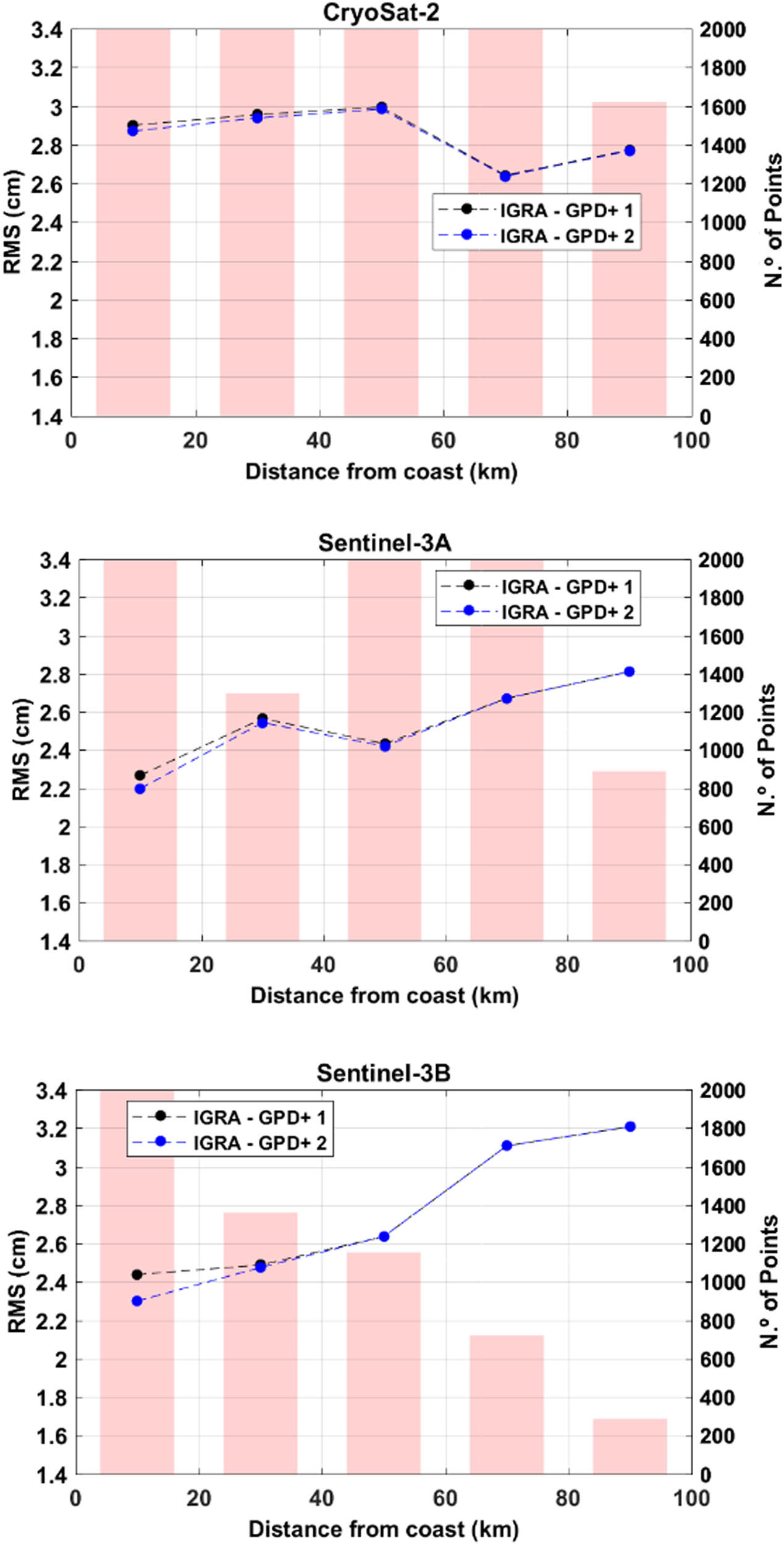
Figure 7a shows the RMS of the differences between WTC from GNSS and each of the two GPD+ solutions for CS2, in centimeters (left axis), and the number of points used (right axis), function of the distance from the coast. This is a non-collocated comparison, which means that the points of interest (points measured by the altimeter) are not located at a single coordinate but are compared with values referring to a single coordinate (GNSS station). This is possible due to the variation of the WTC in space, which extends over a radius of tenths of kilometers (less than 100 km) depending on the variation in each zone (Fernandes and Lázaro, 2016). Then, the GPD+ WTC for altimeter points are compared to the interpolated WTC from GNSS stations for the same time, if they are within a radius of up to 100 km away from the coast, grouped into classes of 5 km (Vieira et al. 2019a).

Figure 7

RMS of differences between GNSS-derived WTC and GPD+ 1 (black) and GPD+ 2 (blue) WTC for (top) CS2, (middle) S3A and (bottom) S3B altimetry points.

It is noticed that the RMS curve of the differences between GNSS and GPD+ 2, in blue, has lower values than the curve of the differences between GNSS and GPD+ 1, in black, up to 70 km from the coast, from which the curves start to overlap. In the opposite direction, the difference between the curves becomes larger as the distance to the coast approaches zero. GPD+ 1 and GPD+ 2 have RMS values around 1.8–2.2 and 1.6–2.2 cm, respectively, from the coast up to a distance of 70 km. This shows that the addition of SIRGAS stations had a positive impact in CS2 estimated WTC, mainly for points close to the coast, achieving a decrease of up to 2 mm in the RMS of the differences with respect to GNSS measurements.

The same analysis was carried out for S3A and S3B with the assessment stations for these satellites, shown in Figure 7b and c, respectively. S3A uses fewer stations in the assessment than CS2, due to the size of its time series and the characteristics of its orbit, and S3B has even fewer points, with even shorter time series than the first two.

For S3A and S3B, it is noticed that the RMS curve of the differences between GNSS and GPD+ 2, in blue, has also lower values than the curve of the differences between GNSS and GPD+ 1, in black, but for both satellites, up to 25 km away from the coast, from which curves start to overlap. This happens because, from this distance on, the GPD+ solution for these satellites already uses valid on-board MWR measurements, which makes the GNSS to have a lower weight on the final estimated value.

It is also noted that the curves of the solutions for S3A and S3B follow the same trend, since these satellites have identical orbital characteristics, but 140° out of phase. The biggest difference is the number of points evaluated, as the S3A was launched two years before S3B.

GPD+ 1 and GPD+ 2 have RMS values around 1.8–2 and 1.6–2 cm, respectively, from the coast up to a distance of 25 km. The impact is mainly for points close to the coast, where GPD+ 1 has values around 1.8 cm, while GPD+ 2 has values around 1.6 cm, achieving a decrease of almost 2 mm in the RMS of the differences with respect to GNSS measurements.

Table 2 shows the number of stations from each network used in the assessment for each satellite. For all satellites, more GPD+ 1 stations were used than SIRGAS-CON stations, which shows that, even with a smaller number of stations, it is already possible to prove the impact of a decrease in the RMS of the WPD differences after using the ZTD from SIRGAS network in GPD+.

Table 2

Number of GNSS stations used in the GPD+ WTC assessment for CS2, S3A and S3B altimetry points

Satellite	Number of IGS and SuomiNet GNSS stations used in the assessment	Number of SIRGAS-CON GNSS stations used in the assessment
CS2	217	144
S3A	200	111
S3B	169	103

In summary, a decrease in the RMS of the differences between GNSS-derived WTC and the GPD+ 2 in relation to the differences with GPD+ 1 was verified for the three satellites, impacting mainly on coastal areas, which are the main target of this study.

6 GPD+ WTC validation with radiosondes

The validation of the densified GPD+ WTC was carried out with radiosondes, which is an external and independent source of information, since it is not an input for GPD+. The radiosondes data are from IGRA, operated by NOAA, and they can be freely downloaded from the webpage https://www.ncei.noaa.gov/products/weather-balloon/integrated-global-radiosonde-archive (NOAA 2022). Radiosondes have a global coverage, as shown in Figure 8 as purple points, and decades of available data.

Figure 8

IGRA network.

The radiosonde observations have a temporal resolution of 24, 12 or 8 h, unlike the SIRGAS-CON ZTD, which have a temporal resolution of 1 h. For this reason, the interpolation for the time of the altimetry points is not adequate, since the radiosonde measurements have a large time gap between them, greater than the WTC variability temporal scale (Vieira et al. 2019c). The altimetry measurements were then selected in a range from −1 to +1 h from each radiosonde measurement instant.

The altimetry points within a distance up to 100 km from the radiosonde were selected. Thus, 78, 13 and 11 radiosondes were selected for the validation of the GPD+ WTC for the altimetry points of CS2, S3A and S3B, respectively. CS2 has a considerably greater number of radiosondes available for the validation due to its orbit, which means that there are more altimetry points within the defined radius. The radiosondes used in the validation for each satellite are shown in Figure 9 represented by different colors: blue points for CS2, red diamonds for S3A and yellow points for S3B.

Figure 9

Radiosondes used in the validation of GPD+ WTC for CS2 (blue points), S3A (red diamonds) and S3B (yellow points).

The same analysis was conducted for radiosondes as in the non-independent assessment with GNSS. The RMS of the differences between WTC from radiosondes and each of the two GPD+ solutions was calculated for CS2, S3A and S3B as a function of distance from the coast. This is also a non-collocated comparison. Then, the GPD+ WTC for altimeter points were compared to the WTC from radiosondes for which the altimeter point was selected, but this time grouped in classes of 20 km to obtain more robust statistics, since there are far fewer radiosondes measurements than GNSS.

Figure 10 shows that the RMS curve of the differences between radiosonde and GPD+ 2, in blue, has lower values than the curve of the differences between GNSS and GPD+ 1, in black, up to 20 km away from the coast for S3A and S3B, from which the curves start to overlap, but not for CS2, for which there is almost no difference between the two curves. The biggest difference is for S3B, which achieves a decrease of 2 mm; however, for S3A and CS2, the difference between the curves is almost zero. This may be related to the distribution of radiosondes used in the validation; since within the study area (area covered by SIRGAS-CON), there is a very large number of radiosondes in the south of the United States, where there was already a high density of GNSS stations in the GPD+ dataset and few SIRGAS-CON stations were added. On the other hand, there is a lower number of radiosondes in South America, mainly on the west coast, where there were few stations in the GPD+ and many SIRGAS-CON stations were added. This softens the impact, especially for CS2, which used more radiosondes located in the northern hemisphere for the validation.

Figure 10

RMS of differences between radiosonde-derived WTC and GPD+ 1 (black) and GPD+ 2 (blue) WTC for (a) CS2, (b) S3A and (c) S3B altimetry points.

For this reason, a local analysis for each radiosonde was carried out to assess which of them had for the selected altimetry points any difference in the RMS of the GPD+ WTC after the inclusion of SIRGAS-CON stations. Figure 11 shows the radiosondes used for CS2 GPD+ WTC validation, in which the radiosondes that had a lower RMS difference after the inclusion of SIRGAS-CON stations, represented by the green diamonds, are mostly located on the east coast of South America, precisely the area where more SIRGAS-CON stations were added and where there are more radiosondes with data available to be used in validation in the southern hemisphere. Oppositely, in the south of the United States, Central America and the Caribbean, there is a lot of blue diamonds, which represent radiosondes where no difference was verified. This is expected, as it was an area already densely covered by IGS and SuomiNet stations, which means that the information added is most of the time redundant. Only one radiosonde had a higher RMS of differences after the inclusion of SIRGAS-CON, located in the Brazilian northeast coast, represented by the red diamond in Figure 11.

Figure 11

Radiosondes with RMS improvement (green diamonds), with no RMS change (blue diamonds) and with RMS degradation (red diamond) for GPD+ 2 WTC in relation to GPD+ 1 WTC for CS2.

To go further into this analysis, the number of former GNSS stations in the GPD+ dataset before the inclusion of SIRGAS-CON stations and the number of SIRGAS-CON stations that were added within a 100 km radius of each radiosonde were counted. Thus, it is possible to analyze the relationship between the behavior of the RMS of the differences with each radiosonde considering the number of former GPD+ stations and the number of added stations.

To perform this analysis, an index was created to measure the impact of SIRGAS-CON stations on the RMS of ZWD differences with radiosondes, where the index value is a ratio given by the number of SIRGAS-CON stations added to GPD+ divided by the number of former GPD+ stations, within a radius of 100 km from the radiosonde. When the number of former GPD+ stations is equal to zero, it is not possible to calculate the ratio, then, particularly in this case, the index assumes the number of added SIRGAS-CON stations (i.e. equivalent to the number of former GPD+ stations equal to 1).

Three cases are possible: (1) index values between 0 and 1 indicate radiosonde locations that have more GPD+ stations than SIRGAS-CON stations in their surroundings; (2) for radiosondes that have more SIRGAS-CON stations added than former GPD+ stations, the index assumes a value greater than 1; or (3) in cases where the number of stations from both networks is the same, the index assumes the value of 1.

In case (1), the difference of RMS does not change or decrease at most 0.1 cm. In case (2), the impact ranges from zero (no impact) to a decrease of up to 0.5 cm. In case (3), the differences of RMS ranges from −0.1 cm (for the only one station represented by the red diamond in Figure 11) to 0.3 cm.

The same analysis was performed for S3A and S3B and shows similar results. Although the number of radiosondes used in the validation of the GPD+ WTC for the altimetry points of these two satellites is about 7 times lower than for CS2, they show similar trends. Only one radiosonde, used in the validation of S3B, had a degradation in the RMS of differences after the inclusion of the SIRGAS-CON stations, corresponding to an RMS increase of 0.1 cm.

Out of a total number of 78 radiosondes for CS2, 13 for S3A and 11 for S3B, 30 had a decrease and only 2 had an increase in the RMS values after the inclusion of SIRGAS-CON stations. It is important to highlight that the majority of the radiosondes that did not have any changes in the RMS are located in areas that are already highly densified in the GPD+ network, making the SIRGAS-CON stations information redundant or not impactful.

The results show that the more SIRGAS-CON stations are added, the lower RMS of the differences with radiosondes than without them. It is also shown that the more GPD+ stations already exist at a given location where SIRGAS-CON stations are added, the less impact the SIRGAS-CON stations have on the WTC GPD+ calculation, and vice versa.

7 Discussion

The main objective of this work was to exploit the GNSS-derived ZWD from SIRGAS-CON, to select and include these stations in the database used by the GPD+ algorithm for the estimation of the WTC for satellite altimetry observations, to improve this correction for the Latin America coastal zones and inland waters.

Considering this purpose, it was expected that the SIRGAS-CON ZWD, derived from their ZTD, would have a good accuracy and stability, compatible with the ZWD derived from IGS network and from ERA5 NWM.

The assessment of the SIRGAS-CON ZWD was carried out by comparisons with the corresponding ZWD from the IGS common stations and with the ZWD computed from the ERA5 model.

Regarding the first comparison, between SIRGAS-CON ZWD and IGS ZWD, a set of 63 stations common to both networks was analyzed. The means of the differences between the two solutions are in a range from −1 to 6 mm, which can be considered an indicator of the good overall quality of the SIRGAS-CON ZWD. Results for the StD of the ZWD differences show values between 3 and 16 mm, with only six of them having values greater than 1 cm. These results are in line with previous studies with similar goals. Fernandes et al. (2013a), aiming to use GNSS-derived tropospheric products in coastal altimetry, performed an analysis of ZTD products using a 7 year time series of 51 IGS and EPN common stations and obtained 2.9 mm in mean and 5.2 mm in StD of the ZTD differences. Mackern et al. (2020) analyzed a 5-year time series of 15 IGS and SIRGAS-CON common stations and obtained a mean bias of −1.5 mm and a mean RMS of 6.8 mm. The same authors obtained similar results in a comparison with radiosondes data, obtaining a mean bias of −2 mm and a mean RMS of 7.5 mm.

The selection of stations to be added to GPD+ was based on a detailed analysis of the differences between SIRGAS-CON ZWD and ERA5 ZWD both computed at the station level.

A total of 366 stations were selected as eligible to be included in GPD+. From a total number of 467 stations with available ZTD, 38 stations were rejected and 63 were not considered in the selection because they are already included in the GPD+ estimations since they are part of the IGS network.

Results show that, overall, there is a decrease in the RMS of the differences between GNSS-derived WTC and the GPD+ solution after the addition of the SIRGAS-CON stations when compared to the differences with the previous solution, for the three evaluated satellite altimetry points. The impact is greater at the points closer to the coast, reaching a 2 mm decrease in RMS, extending up to 25 km away from the coast for points in S3A and S3B, while for CS2, this impact is up to 70 km. This happens due to the characteristics of GPD+ processing for CS2, which does not use on-board MWR measurements as input. MWR start to fail when they reach approximately 30 km away from the coast, therefore, for longer distances, valid MWR measurements are already used for S3A and S3B, reducing the weight of GNSS observations in the GPD+ estimations for these satellites.

An independent validation with radiosondes was also carried out and the results show an improvement for the study region, especially for S3B, for altimetry points up to 20 km away from the coast. The RMS analysis of the points grouped in categories of distance away from the coast did not present significant results for the S3A and CS2 satellites; therefore, a local analysis, just for the points within a radius of 100 km of distance from each radiosonde, was performed.

In this analysis, it is possible to notice that there is an improvement in the RMS values, especially in the points around radiosondes where more SIRGAS-CON stations were added and where there were fewer former GPD+ stations. The decrease in RMS reaches up to 0.5 cm for some radiosondes. The results of this validation are in agreement with the GNSS non-independent assessment performed previously and reinforce the conclusion that SIRGAS-CON stations improve GPD+, thus achieving the proposed objective of this work.

The intention is to continue the exploitation of other regional networks in the future, in regions of the planet that still lack WTC observations, to improve the GPD+ performance also in these regions. Southeast Asia, Japan and Oceania, regions characterized by the presence of many islands, are prone to MWR failure and still have few GNSS stations in the GPD+ database; thus, a densification in these regions is needed to improve WTC in their coastal zones. The African continent, in addition to having one of the most extensive coast in the world, has large inland water bodies, such as Lake Victoria and Lake Tanganyika, but it has very few GNSS stations in its territory.

It is also expected that more stations will be added to existing networks and that new networks will be created in the future; then, there will be a good coverage of GNSS stations in all regions of the planet, which will provide more information to improve the WTC estimation and consequently satellite altimetry products.

Acknowledgements

The authors would like to thank two anonymous reviewers for their constructive comments and discussions. We thank ESA’s HYDROCOASTAL project for providing the funding for this work. We acknowledge the data from IGS, SIRGAS, ECMWF and NOAA IGRA.

Conflict of interest: Authors state no conflict of interest.

References

Bevis, M., S. Businger, S. Chiswell, T. A. Herring, R. A. Anthes, C. Rocken, et al. 1994. “GPS meteorology: Mapping zenith wet delays onto precipitable water.” Journal of Applied Meteorology and Climatology 33(3), 379–386. http://www.jstor.org/stable/26186685.10.1175/1520-0450(1994)033<0379:GMMZWD>2.0.CO;2Search in Google Scholar

Bevis, M., S. Businger, T. A. Herring, C. Rocken, R. A. Anthes, and R. H. Ware. 1992. “GPS meteorology: Remote sensing of atmospheric water vapor using the Global Positioning System.” Journal of Geophysical Research: Atmospheres 97(D14), 15787–15801. 10.1029/92JD01517.Search in Google Scholar

Boehm, J. and H. Schuh. 2004. “Vienna mapping functions in VLBI analyses.” Geophysical Research Letters 31, L01603. 10.1029/2003GL018984.Search in Google Scholar

Boehm, J., B. Werl, and H. Schuh. 2006a. “Troposphere mapping functions for GPS and very long baseline interferometry from European Centre for Medium-Range Weather Forecasts operational analysis data.” Journal of Geophysical Research 111, B02406, 10.1029/2005JB003629.Search in Google Scholar

Boehm, J., A. Niell, P. Tregoning, and H. Schuh. 2006b. “Global Mapping Functions (GMF): A new empirical mapping function based on numerical weather model data.” Geophysical Research Letters 33, L07304, 10.1029/2005GL025546.Search in Google Scholar

Böhm, J., R. Heinkelmann, and H. Schuh. 2007. “Short note: a global model of pressure and temperature for geodetic applications.” Journal of Geodesy 81(10), 679–683. 10.1007/s00190-007-0135-3.Search in Google Scholar

Brown G. 1977. “The average impulse response of a rough surface and its applications.” IEEE Transactions on Antennas and Propagation 25(1), 67–74. 10.1109/TAP.1977.1141536.Search in Google Scholar

Camisay M. F., J. A. Rivera, M. L. Mateo, P. V. Morichetti, and M. V. Mackern. 2020, Estimation of integrated water vapor derived from Global Navigation Satellite System observations over Central-Western Argentina (2015–2018). Validation and usefulness for the understanding of regional precipitation events. Journal of Atmospheric and Solar-Terrestrial Physics 197, 105143. 10.1016/j.jastp.2019.105143.Search in Google Scholar

Chelton D. B., J. C. Ries, B. J. Haines, L. L. Fu, and P. S. Callahan. 2001. Satellite altimetry. In Satellite Altimetry and Earth Sciences: A Handbook of Techniques and Applications, edited by L. L. Fu, A. Cazenave. San Diego, CA, USA: Academic, Vol. 69, p. 1–131.10.1016/S0074-6142(01)80146-7Search in Google Scholar

Davis, J. L., T. A. Herring, I. I. Shapiro, A. E. E. Rogers, and G. Elgered. 1985. “Geodesy by radio interferometry: Effects of atmospheric modeling errors on estimates of baseline length.” Radio Science 20(6), 1593–1607. 10.1029/RS020i006p01593.Search in Google Scholar

Dee, D. P., S. M. Uppala, A. J. Simmons, P. Berrisford, P. Poli, S. Kobayashi, et al. 2011. “The ERA‐Interim reanalysis: Configuration and performance of the data assimilation system.” Quarterly Journal of the Royal Meteorological Society 137(656), 553–597. 10.1002/qj.828.Search in Google Scholar

European Centre for Medium-Range Weather Forecasts “ECMWF”, 2021. http://www.ecmwf.int/.Search in Google Scholar

Fernandes, M. J. and C. Lázaro. 2016. “GPD + wet tropospheric corrections for CryoSat-2 and GFO altimetry missions.” Remote Sensing 8(10), 851. 10.3390/rs8100851.Search in Google Scholar

Fernandes, M. J., C. Lázaro, M. Ablain, and N. Pires. 2015. “Improved wet path delays for all ESA and reference altimetric missions.” Remote Sensing of Environment 169, 50–74. 10.1016/j.rse.2015.07.023.Search in Google Scholar

Fernandes, M. J., N. Pires, C. Lázaro, and A. L. Nunes. 2013a. “Tropospheric delays from GNSS for application in coastal altimetry.” Advances in Space Research 51(8), 1352–1368. 10.1016/j.asr.2012.04.025.Search in Google Scholar

Fernandes, M. J., C. Lázaro, A. L. Nunes, N. Pires, L. Bastos, and V. B. Mendes. 2010. “GNSS-derived path delay: An approach to compute the wet tropospheric correction for coastal altimetry.” IEEE Geoscience and Remote Sensing Letters 7(3), 596–600. 10.1109/LGRS.2010.2042425.Search in Google Scholar

Fernandes, M. J., C. Lázaro, A. L. Nunes, and R. Scharroo. 2014. “Atmospheric corrections for altimetry studies over inland water.” Remote Sensing 6(6), 4952–4997. 10.3390/rs6064952.Search in Google Scholar

Fernandes, M. J., C. Lázaro, and T. Vieira. 2021a. “On the role of the troposphere in satellite altimetry.” Remote Sensing of Environment 252, 112149. 10.1016/j.rse.2020.112149.Search in Google Scholar

Fernandes, M. J., C. Lázaro, and T. Vieira. 2021b. “WP2310, Wet Tropospheric Correction Dry Tropospheric Correction (CCN1).” HYDROCOASTAL Sentinel-3 and Cryosat SAR/Sarin Radar Altimetry For Coastal Zone and Inland Water, Second Progress Meeting, Video Conference, 4th February 2021.Search in Google Scholar

Geodetic Reference System for the Americas “SIRGAS”, 2021. https://sirgas.ipgh.org/.Search in Google Scholar

Ghoddousi-Fard, R. 2009. “Modelling tropospheric gradients and parameters from NWP models: effects on GPS estimates.” Ph.D. dissertation, Univ. of New Brunswick, Canada.Search in Google Scholar

Gommenginger, C., P. Thibaut, L. Fenoglio-Marc, G. Quartly, X. Deng, J. Gómez-Enri, et al. 2011, “Retracking altimeter waveforms near the coasts.” Coastal Altimetry, 61–101. 10.1007/978-3-642-12796-0_4.Search in Google Scholar

Hersbach, H., B. Bell, P. Berrisford, G. Biavati, A. Horányi, J. Muñoz Sabater, et al. 2018. ERA5 hourly data on single levels from 1979 to present, Copernicus Climate Change Service (C3S) Climate Data Store (CDS), 10. 10.24381/cds.adbb2d47.Search in Google Scholar

Hopfield, H. S. 1969. “Two‐quartic tropospheric refractivity profile for correcting satellite data.” Journal of Geophysical Research 74(18), 4487–4499. 10.1029/JC074i018p04487.Search in Google Scholar

Kouba, J. 2008. “Implementation and testing of the gridded Vienna Mapping Function 1 (VMF1).” Journal of Geodesy 82(4), 193–205. 10.1007/s00190-007-0170-0.Search in Google Scholar

Lázaro, C. and M. J. Fernandes. 2015. “An enhanced MWR-based wet tropospheric correction for Sentinel-3: inheritance from past ESA altimetry missions.” In Sentinel-3 for Science Workshop Vol. 734, p. 25.Search in Google Scholar

Lázaro, C., M. J. Fernandes, T. Vieira, and E. Vieira. 2020. “A coastally improved global dataset of wet tropospheric corrections for satellite altimetry.” Earth System Science Data 12(4), 3205–3228. 10.5194/essd-12-3205-2020.Search in Google Scholar

Mackern, M. V., M. L. Mateo, M. F. Camisay, and P. V. Morichetti. 2020. “Tropospheric products from high-level GNSS processing in Latin America.” International Association of Geodesy Symposia. 10.1007/1345_2020_121.Search in Google Scholar

Mackern, M. V., M. L. Mateo, M. F. Camisay, P. A. Rosell, T. Weidmann, and A. Gonzalez Romo. 2021. “Análisis del modelo de cálculo utilizado para obtener el vapor de agua troposférico desde los retardos en la señal gnss en la región centro oeste de Argentina.” ICU - Investigación, Ciencia y Universidad 5, 14–30. http://revistas.umaza.edu.ar/index.php/icu/article/view/344.Search in Google Scholar

Mendes, V. B. 1999. “Modeling the neutral-atmospheric propagation delay in radiometric space techniques.” UNB Geodesy and Geomatics Engineering Technical Report 199, 10.Search in Google Scholar

Mendes V. B., G. Prates, L. Santos, and R. B. Langley. 2000. “An evaluation of the accuracy of models for the determination of the weighted mean temperature of the atmosphere.” In Proceedings of the 2000 National Technical Meeting of The Institute of Navigation, pp. 433–438.Search in Google Scholar

Miller, M., R. Buizza, J. Haseler, M. Hortal, P. Janssen, and A. Untch. 2010. “Increased resolution in the ECMWF deterministic and ensemble prediction systems.” ECMWF Newsletter, 124, 10-16. 10.21957/kyhds35r.Search in Google Scholar

Niell, A. E. 1996, “Global mapping functions for the atmosphere delay at radio wavelengths.” Journal of Geophysical Research 101, 3227–3246. 10.1029/95JB03048.Search in Google Scholar

Niell, A. E., A. J. Coster, F. S. Solheim, V. B. Mendes, P. C. Toor, R. B. Langley, et al. 2001. “Comparison of measurements of atmospheric wet delay by radiosonde, water vapor radiometer, GPS, and VLBI.” Journal of Atmospheric and Oceanic Technology 18(6), 830–850. 10.1175/1520-0426(2001)018<0830:COMOAW > 2.0.CO;2.Search in Google Scholar

National Oceanic and Atmospheric Administration “NOAA”, 2022. https://www.ncei.noaa.gov/products/weather-balloon/integrated-global-radiosonde-archive.Search in Google Scholar

Notarpietro, R., M. Cucca, M. Gabella, G. Venuti, and Perona G. 2011. “Tomographic reconstruction of wet and total refractivity fields from GNSS receiver networks.” Advances in Space Research 47, 898–912. 10.1016/j.asr.2010.12.025.Search in Google Scholar

Pacione, R., B. Pace, H. Vedel, S. De Haan, R. Lanotte, and F. Vespe. 2011. “Combination methods of tropospheric time series.” Advances in Space Research 47(2), 323–335. 10.1016/j.asr.2010.07.021.Search in Google Scholar

Stum, J., P. Sicard, L. Carrere, and J. Lambin. 2011. “Using objective analysis of scanning radiometer measurements to compute the water vapor path delay for altimetry.” IEEE Transactions on Geoscience and Remote Sensing 49(9), 3211–3224. 10.1109/TGRS.2011.2104967.Search in Google Scholar

Vieira, T., M. J. Fernandes, and C. Lázaro. 2018. “Independent assessment of on-board microwave radiometer measurements in coastal zones using tropospheric delays from GNSS.” IEEE Transactions on Geoscience and Remote Sensing 57(3), 1804–1816. 10.1109/TGRS.2018.2869258.Search in Google Scholar

Vieira, E., C. Lázaro, and M. J. Fernandes. 2019c. “Spatio-temporal variability of the wet component of the troposphere–application to satellite altimetry.” Advances in Space Research 63(5), 1737–1753. 10.1016/j.asr.2018.11.015.Search in Google Scholar

Vieira, T., M. J. Fernandes, and C. Lazaro. 2019b. “Impact of the new ERA5 reanalysis in the computation of radar altimeter wet path delays.” IEEE Transactions on Geoscience and Remote Sensing 57(12), 9849–9857. 10.1109/TGRS.2019.2929737.Search in Google Scholar

Vieira, T., M. J. Fernandes, and C. Lázaro. 2019a. Modelling the altitude dependence of the wet path delay for coastal altimetry using 3-D fields from ERA5 Remote Sensing 11(24), 2973. 10.3390/rs11242973.Search in Google Scholar

Thayer, G. D. 1974. “An improved equation for the radio refrative index of air.” Radio Science 9(10), 803–807. 10.1029/RS009i010p00803.Search in Google Scholar

Tregoning, P. and T. A. Herring. 2006. “Impact of a priori zenith hydrostatic delay errors on GPS estimates of station heights and zenith total delays.” Geophysical Research Letters 33, L23303. 10.1029/2006GL027706.Search in Google Scholar

Yang, L., Z. Elmas, C. Hill, M. Aquino, and T. Moore. 2011. “An Innovative Approach for Atmospheric Error Mitigation Using New GNSS Signals.” The Journal of Navigation 64, S211–S232. 10.1017/S0373463311000373.Search in Google Scholar

Received: 2022-02-28

Revised: 2022-11-23

Accepted: 2022-11-24

Published Online: 2022-12-23

This work is licensed under the Creative Commons Attribution 4.0 International License.

Articles in the same Issue

https://doi.org/10.1515/jogs-2022-0146

Keywords for this article

coastal zones; CryoSat-2; GNSS; Latin America; microwave radiometer; radiosonde; Sentinel-3; troposphere; water vapor

Creative Commons

BY 4.0