Low-frequency fluctuations in the yearly misclosures of the global mean sea level budget during 1900–2018
-
H. Bâki Iz


Abstract
Sub- and super-harmonics of luni-solar forcing are proxies for the natural variations in sea levels observed at tide gauge stations with long records as demonstrated in earlier studies. This study also identified their signatures in the noisy yearly misclosures of the global mean sea level budget for the period 1900–2018. The analyses of the yearly misclosures revealed a temporal linear systematic error of 0.08 ± 0.02 mm/year, which is not explained by the budget components. The estimate is statistically significant (α = 0.05) but small in magnitude and accounts for only 11% (adjusted R 2) of the variations in the yearly misclosures. Meanwhile, the yearly misclosures have also a statistically significant constant bias as large as −12.2 ± 0.9 mm, which can be attributed to the lack of a common datum definition for the global mean sea level budget components. Modeling the low-frequency changes of luni-solar origin together with a trend and constant bias parameters reduces variability in the misclosures. Accounting for their effects explains 50% (adjusted R 2) of the fluctuations in the yearly misclosures compared to the 11% if they are not. In addition, unmodeled low-frequency variations in the yearly global budget closure assessments have the propensity of confounding the detection of a statistically significant recent uniform global sea level acceleration triggered by anthropogenic contributors.
Science and philosophy are all about categorizing things better, and that often means making new and finer distinctions.
Julian Baggini 2009 The Duck that won the lottery.
1 Introduction
Sea level variations are driven by various effects and are very noisy due to seasonal, interannual, decadal, and longer variations of the ocean surface (Cazenave and Remy 2011). Sea level rise at long time scales is attributed to ocean thermal expansion and halosteric contraction, ice sheet, mountain glacier and ice cap mass balance, changes in terrestrial surface and ground water storage, and anthropogenic impoundment of waters in dams. To much lesser importance, permafrost degradation and snow and atmospheric water vapor change are also identified as major geophysical contributors to the present-day global mean sea level (GMSL) rise (Moore et al. 2011, Gregory et al. 2013, Slangen et al. 2017, Cazenave et al. 2018, WCRP Global Sea Level Budget Group 2018, Iz et al. 2018, Iz and Shum 2020a,b,c, Frederikse et al. 2020, Horwath et al. 2022).
The recent study by Frederikse et al. (2020) compiled yearly time series of GMSL budget components during 1900–2018 together with their error estimates, which are essential for proper analyses of the GMSL budget misclosures.[1] They also reported 0.04 ± 0.22 mm/year misclosure rate[2] calculated from the root sum of squares (RSSQ) of the GMSL budget components’ velocities and their uncertainties. Although the reported misclosure rate is small in magnitude, its uncertainty is as large as the velocities of some of the budget components. Meanwhile, yearly GMSL misclosures exhibit periodic fluctuations at different time scales unexplained by the budget components as it will be shown in this study. They are interannual, decadal, and multidecadal scales and multicausal due to the natural forcing such as temperature, wind and pressure, or ocean circulations, which could be conflated and/or excited externally by astronomical forcing. They are usually identified as broadband processes in the context of wind-induced decadal variability (Sturges and Hong 2001) as well as the signatures oceanic and atmospheric transport of multiyear El Niño–Southern Oscillation to the polar regions. The periodic components of the decadal sea level variations were also reported by a number of studies (Häkkinen 2000, Ünal and Ghil 1995, Jevrejeva et al. 2004).
Selected compounded luni-solar periods in years
| Nodal and supe-harmonics | Nodal sub-harmonics | Solar and super-harmonics |
|---|---|---|
| 18.6 | 18.6/2 = 9.3 | 11.1 |
| 18.6 × 2 = 37.2 | 18.6/3 = 6.2 | 11.1 × 2 = 22.2 |
| 18.6 × 3 = 55.8 | ||
| 18.6 × 4 = 74.5 |
Keeling and Whorf (1997) proposed realization of luni-solar forcing in conjunction with random beats of nearby natural and/or forced broadband oscillations of the sea level at multidecadal and decadal frequencies. Munk et al. (2002) suggested compounding of periodic lunar nodal tides and almost periodic solar radiation variations with natural variations in sea level inciting periodic oscillations of the sea level at multidecadal and decadal frequencies (super-harmonics). Their effects are also realized at interannual time scales through their sub-harmonics. Stationary long-period tides introduce vertical temperature mixing between sea surface temperature and cold bottom temperatures, thereby the source of global thermosteric sea level changes (Yndestad 2021).
A meta-analysis of the long tide gauge (TG) records by Iz (2014) revealed the compounding effect of luni-solar forcing (acting as carrier frequencies) at a global scale in TG records. Regardless of their origins, sub- and super-harmonic of periodic sea-level variations are proxies in representing natural fluctuations in the sea level effectively. Subsequent studies by Iz (2015, 2016a,b) produced further observational evidence for their presence. These periodic anomalies in the sea level propagate into the GMSL budget misclosures preponderantly through the observed GMSL time series.
Although the presence of luni-solar forcing in sea-level fluctuations has been well studied by this investigator through analyses of long TG records individually, the availability of the newly compiled records of the budget components spanning over a century offers an opportunity to verify the earlier findings. Hence, this study aims to model and investigate fluctuations in GMSL budget misclosures for the signatures of luni-solar sub- and super-harmonics at the global scale during 1900–2018.
In the following sections, first, the time series for the GMSL budget components compiled by Frederikse et al. (2020) are presented with their errors. The yearly time series of the budget components are used to calculate yearly GMSL budget misclosures (will be stated onward as misclosures for brevity) and their errors through variance propagation. Subsequently, the systematic errors in the yearly misclosures are represented by a basic kinematic model with a trend (velocity) and a uniform acceleration. This model is to serve as a baseline for assessing the explanatory power of the subsequent models that incorporate the proxy periodicities due to the compounding of luni-solar forcing with natural sea-level variations with and without the uniform acceleration. The statistics of each model solution are tabulated for comparison, and the numerical assessment of the explanatory contributions of the model parameters to the yearly misclosures is made.
2 Data on yearly variations of the GMSL budget components
The data compiled by Frederikse et al. (2020) rely on earlier work cited in their article. Figures 1–6 display the yearly variations of the GMSL budget components during 1900–2018 for a total of 119 yearly averaged values for each one of the GMSL budget components, together with their uncertainties (1 SE), which are expressed in mm of equivalent sea level during this period. The yearly time series are accessible online. The availability of the errors of the time series spanning 1900–2018 is a major contribution of their study for proper formalism in assessing GMSL budget misclosures.

Yearly averaged anomalies of GMSL and their a priori uncertainties (SE) during 1900–2018 (Frederikse et al. 2020).

Yearly averaged anomalies of Glaciers component and their a priori uncertainties (SE) during 1900–2018 (Frederikse et al. 2020).

Yearly averaged anomalies of Greenland component and their a priori uncertainties (SE) during 1900–2018 (Frederikse et al. 2020).

Yearly averaged Steric anomalies and their a priori uncertainties (SE) during 1900–2018 (Frederikse et al. 2020).

Yearly averaged anomalies of Antarctic component and their a priori uncertainties (SE) during 1900–2018 (Frederikse et al. 2020).

Yearly averaged anomalies of terrestrial water storage (TWS) component and their a priori uncertainties (SE) during 1900–2018 (Frederikse et al. 2020).
The condition equations for assessing the closure/misclosure of the GMSL budget using these time series are discussed in the following section. The formulation enables the calculation of the yearly misclosures and their uncertainties through variance propagation.
3 The GMSL sea-level budget and its yearly misclosure statistics
Following the narratives by WCRP Global Sea Level Budget Group (2018), Iz et al. (2019), Iz and Shum (2020a,b), the GMSL budget closure is formulated as follows:
where
The GMSL budget misclosure is quantified yearly using annually and globally averaged sea-level height anomalies of each component,
where superscript t is the epoch of the yearly averaged anomaly. The yearly misclosures are the lump sum effect of the potential systematic errors and the random noise in the yearly averaged time series of the budget components (commission errors) as well as any other unknown contributors (omission errors) shown in Figure 7. The same figure includes the standard errors of the misclosures on a yearly basis calculated from the known yearly SE of the budget components using variance propagation through equation (2)[3]. Its root weighted sum of squares[4] is 10.02 mm and the weighted mean of misclosures is

Yearly misclosures and their uncertaintainties (1 SE) calculated through variance propagation using equation (2). The weighted sum of squares of the yearly budget misclosures is

The yearly averaged anomalies of GMSL budget components with their 1 SE uncertainties. The yearly misclosures are shown with their uncertainties in gray color.
4 The GMSL sea-level budget closure assessed using the trends of its budget components
The time derivative of the yearly budget component given by equation (2) can be expressed as follows:
In this relationship, v refers to the linear trend, constant velocity of a budget component and v
W
is the misclosure rate. The budget misclosure rates will be quantified in the following sections. Recent studies WCRP Global Sea Level Budget Group (2018) and Frederikse et al. (2020) already reported some estimates on this topic. The former study’s rate
The magnitude of the misclosure rate from the WCRP Global Sea Level Budget Group (2018) study is large and uncertain. The findings of Frederikse et al. (2020) GMSL budge misclosure rate is markedly improved. However, its error estimate is still as large as the magnitude of some of the velocities of the budget components.
In the following section, yearly fluctuations in the budget misclosures are modeled and estimated together with their uncertainties using weighted least squares (WLS) method (Mardia et al. 1979) to provide an alternative approach in assessing GMSL budget misclosures.
5 Model I – Yearly variations in GMSL budget misclosures with a linear trend
Given the time evolution of the misclosures, W
t
, in Figure 7, a basic representation of a potential linear temporal systematic error
In this expression, W
0 represents the constant datum offset, which is referenced to the middle of the series, and W
t
is the yearly misclosure at an epoch t. The noise
WLS solution statistics that account for the uncertainties of the misclosures[6] for this model are tabulated in Table 2. The residuals of the misclosures after the adjustment are shown in Figure 9. They exhibit stark unmodeled random excursions over time. The AR(1) autocorrelation coefficient of the residuals,
The RSSQ of misclosure of the budget component velocities and the solution statistics for four different models are tabulated. The unit for the velocity and uniform acceleration are in mm/year and mm/year2, respectively. The units of all other estimates are represented in mm. Adj. R 2 is represented in percent. RSSQ velocity misclosure is quoted from the study by Frederikse et al. (2020)
| Models | RSSQ | Model I | Model II | Model III | Model IV | |||||||||
|---|---|---|---|---|---|---|---|---|---|---|---|---|---|---|
| p |
|
SE |
|
SE | VIF |
|
SE | VIF |
|
SE | VIF |
|
SE | VIF |
| W 0 | −3.43 | 0.82 | −6.51 | 0.84 | −10.83 | 1.03 | −8.51 | 0.68 | −12.20 | 0.90 | ||||
| v W | 0.04 | 0.22a | 0.09 | 0.02 | 1.0 | 0.04 | 0.02 | 1.2 | 0.08 | 0.02 | 1.3 | 0.08 | 0.02 | 1.4 |
| a W | 0.008 | 0.001 | 1.2 | 0.011 | 0.001 | 1.4 | ||||||||
| C75 | −10.03 | 1.18 | 1.8 | NS | NS | NS | ||||||||
| S56 | 3.41 | 0.94 | 1.3 | 3.38 | 0.94 | 1.3 | ||||||||
| C56 | 7.23 | 1.03 | 1.7 | NS | NS | NS | ||||||||
| S37 | −3.98 | 0.88 | 1.2 | −3.51 | 0.84 | 1.1 | ||||||||
| C37 | NS | NS | 3.84 | 0.86 | 1.2 | |||||||||
| C22 | NS | NS | 2.57 | 0.81 | 1.1 | |||||||||
| S18.6 | 1.73 | 0.81 | 1.0 | NS | NS | NS | ||||||||
| RMSE | 10.0 | 2.5 | 2.2 | 1.9 | 1.9 | |||||||||
| Adj. R 2 % | 11.2 | 32.8 | 48.8 | 50.5 | ||||||||||
aThe SE of the estimate was reconstructed from the reported confidence interval (CI) at

Misclosure residuals (mm) of the WLS solution to the trend-only model.
The estimated misclosure velocity (trend/bias)
5.1 Model II – Yearly variations in GMSL sea-level budget misclosures with a linear trend and a uniform acceleration
The trend bias examined in the previous section is a poor representation of yearly variations of the misclosures (Adj. R 2 = 11%). Although there is no visual evidence for a potential uniform acceleration in the misclosure residuals (Figure 9), claims were made by recent studies (e.g., Hogarth 2014) about its presence in GMSL anomalies during this period. Examining its presence will therefore be informative. The new model reads as follows:
In this model, the uniform acceleration parameter is defined as
Another WLS solution was carried out for using this model. The solution statistics are tabulated in Table 2 under Model II. The impact of the uniform acceleration parameter is substantial. It increased the explanatory power of the model by threefold (Adj. R
2 = 32.8%) compared to the Model I representation (Adj. R
2 = 11.2%). The estimated uniform acceleration is also statistically significant
Also, the misclosure trend estimate is identical to the one reported by Frederikse et al. (2020), and its uncertainty has improved by an order of magnitude, i.e.,
5.2 Model III – Yearly variations in of GMSL sea-level budget misclosures with a linear trend, luni-solar forcing, and their sub- and super-harmonics
Interannual, decadal, and multi-decadal fluctuations are recognized and attributed to natural variations in GMSL (e.g., Bindoff et al. 2007, Llovel et al. 2011, Esselborn et al. 2018, Dieng et al. 2021). As elucidated in Section 1, luni-solar forcing and their sub- and super-harmonics are realized as proxies representing the combined effect of natural sea-level variations (Iz 2014). If these proxies are not modeled, they will propagate into the budget misclosures through the GMSL time series. Therefore, they must be accounted for in assessing the GMSL budget closure. The following model for the GMSL budget misclosures is a kinematic representation, inclusive of periodic variations of luni-solar origin:
Modeling periodicities introduces additional two parameters,
The estimated parameters obtained using WLS solutions for equation (6) are tabulated in Table 2 under Model III. The listed estimates are all statistically significant at
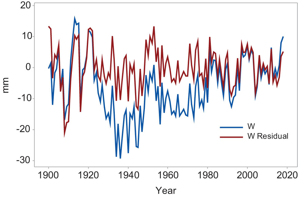
Misclosures and misclosure residuals are displayed. The RMS of the misclosures = 10.0 mm, reduced to 1.9 mm (the RMSE of the misclosure residuals) after modeling the linear trend and the periodic variations due to the luni-solar forcing.
The variance inflation factors (VIFs) of the estimated parameters indicate that they are well separated, i.e., uncorrelated. The random nature of the misclosure residuals is confirmed by their normal probability plot shown in Figure 11.

Misclosure residuals (mm) vs expected normal distribution (red).
As stated earlier, the nonlinear progression of the GMSL rise displayed in Figure 1 also suggests a uniform acceleration during this period. Several studies such as Dangendorf et al. (2017, 2019) and Nerem et al. (2018) reported a statistically significant uniform acceleration during 1993–2018. Nonetheless, Iz and Shum (2020d) demonstrated that the signature of the claimed uniform acceleration is ambiguous since it can also be attributed to low-frequency sea-level variations, mainly caused by compounding of luni-solar forcing with natural sea-level changes and cannot be detected using short Satellite Altimetry (SA) time series. Given the availability of the series of the GMSL budget components spanning over a century offers an opportunity to resolve this ambiguity. Therefore, parameters of equation (6) are estimated together with an added uniform acceleration parameter.
5.3 Model IV – Yearly variations in GMSL sea-level budget misclosures with a constant velocity, uniform acceleration, luni-solar forcings, and their sub- and super-harmonics
The model augmented with the uniform acceleration has the same descriptions for the parameters stated in the previous section and reads as follows:
The estimated parameters and their statistics are again obtained using WLS and listed in Table 2 under Model IV. The estimates are all statistically significant at
6 Discussion and conclusion
This study quantified the yearly GMSL budget misclosures during 1900–2018 using different kinematic models and detected a linear temporal systematic error of 0.08 ± 0.02 mm/year, which is statistically significant but negligible in size compared to the trends of the budget components. However, yearly misclosures have a statistically significant constant error of varying magnitudes estimated by the models entertained in this study. This constant error is labeled as datum bias, and therefore, the yearly GMSL budget cannot be claimed as closed. The physical implication of this constant bias is unbeknown to this investigator and further investigation about its origin may be needed.
More importantly, the current uncertainties of yearly misclosures (commission errors) are large for an effective yearly budget closure and were explained by the major findings of this study. The dominant systematic portion of these fluctuations are due to the periodicities induced by luni-solar forcing and their super- and sub-harmonics in the GMSL budget during 1900–2018. A similar finding was already reported by Iz (2014) in globally distributed individual TG stations with long records. Modeling the effect of the low-frequency fluctuations together with the trend and datum bias explained up to 50% (Adj. R 2) of the fluctuations in GMSL misclosures compared to the 11% in their absence. The low-frequency fluctuations have the propensity of confounding the detection of a uniform global sea-level acceleration that may have been caused by anthropogenic contributors (Iz and Shum 2020d). Taking their effects into account in GMSL budget misclosures is therefore a necessity not only for closure but also for accurate predictions of future global sea-level variations as part of climate change projections (Iz and Shum 2020c).
A by-product of this study is about the presence of a uniform GMSL acceleration during the SA era, 1993 onward, claimed by Nerem et al. (2018), whose certitude is challenged by Iz and Shum (2020d). The topic has important ramifications for understanding recent anthropogenic contributions of the global warming and its impact on sea levels and mitigation efforts. The availability of the budget data spanning 1900–2018 and, in particular, the availability of their uncertainties provided an opportunity to investigate this claim through the yearly misclosures of the GMSL budget components. Unfortunately, the models with and without a uniform acceleration (Model III and Model IV) during this period still cannot establish the presence or the absence of a global uniform acceleration during this period. On the one hand, if the extended time span of the data suggests that there is no uniform acceleration during this period (Model III), then there cannot be a uniform acceleration during SA era either since both data sets overlap. On the other hand, if the acceleration is uniform going back to 1900 as Model IV suggests, then the acceleration during the SA era is not a recent phenomenon as claimed by the proponents for its recency.
In any event, the aforementioned discussion should not be construed as a climate change skepticism but a question for further investigation. Although the estimated trend misclosures are robust for the models entertained in this study, the periodic low-frequency variations and more importantly the absence or presence of a uniform acceleration will lead to substantially different predictions of the GMSL rise (İz 2022) and is consequential for climate change mitigation measures.
Acknowledgments
Constructive comments of the two anonymous reviewers improved the manuscript. Their contributions are greatly appreciated. This study was supported by Natural Science Foundation of China (41974040).
-
Conflict of interest: Author states no conflict of interest.
References
Baggini, J. 2009. The duck that won the lottery: 100 New experiments for the armchair philosopher. Plume Publisher, New York.Search in Google Scholar
Bindoff, N. L., J. Willebrand, V. Artale, A. Cazenave, J. Gregory, S. Gulev, et al. 2007. “Observations: oceanic climate change and sea level.” In: Climate Change 2007: The Physical Science Basis. Contribution of Working Group I to the Fourth Assessment Report of the Intergovernmental Panel on Climate Change, edited by Solomon, S., D. Qin, M. Manning, Z. Chen, M. Marquis, K. B. Averyt, M. Tignor and H. L. Miller. Cambridge University Press, Cambridge, United Kingdom and New York, NY, USA.Search in Google Scholar
Cazenave, A., B. Meyssignac, M. Ablain, M. Balmaseda, J. Bamber, V. Barletta, et al. 2018. “Global sea-level budget 1993-present.” Earth System Science Data 10(3), 1551–90. 10.5194/essd-10-1551-2018.Search in Google Scholar
Cazenave, A. and F. Remy. 2011. “Sea level and climate: Measurements and causes of changes.” Interdisciplinary Reviews: Climate Change 2(5), 647–62. 10.1002/wcc.139.Search in Google Scholar
Dangendorf, S., M. Marcos, G. Wöppelmann, C. P. Conrad, T. Frederikse, R. Riva. 2017. “Reassessment of 20th century global mean sea level rise.” Proceedings of the National Academy of Sciences of the United States of America 114(23), 5946–51. 10.1073/pnas.1616007114.Search in Google Scholar
Dangendorf, S., C. Hay, F. M. Calafat, M. Marcos, C. G. Piecuch, K. Berk, et al. 2019. “Persistent acceleration in global sea-level rise since the 1960s.” Nature Climate Change, 9(9), 705–10. 10.1038/s41558-019-0531-8.Search in Google Scholar
Dieng, H. B., A. Cazenave, Y. Gouzenes, and B. A. Sow. 2021. “Trends and inter-annual variability of altimetry-based coastal sea level in the Mediterranean Sea: Comparison with tide gauges and models.” Advances in Space Research. 68(8), 3279–90, ISSN 0273-1177, https://doi.org/10.1016/j.asr.2021.06.022.10.1016/j.asr.2021.06.022Search in Google Scholar
Esselborn, S., S. Rudenko, and T. Schöne. 2018. “Orbit-related sea level errors for TOPEX altimetry at seasonal to decadal timescales.” Ocean Science 14, 205–23. 10.5194/os-14-205-2018.Search in Google Scholar
Frederikse, T., F. Landerer, L. Caron, S. Adhikari, D. Parkes, V. W. Humphrey, et al. 2020. “The causes of sea-level rise since 1900.” Nature 584, 393–7.10.1038/s41586-020-2591-3Search in Google Scholar
Gregory, J. M., N. J. White, J. A. Church, M. F. P. Bierkens, J. E. Box, M. R. Van den Broeke, et al. 2013. “Twentieth-century global-mean sea level rise: Is the whole greater than the sum of the parts?.” Journal of Climate 26(13), 4476–99. 10.1175/JCLI-D-12-00319.1.Search in Google Scholar
Häkkinen, S. 2000. “Decadal Air–Sea Interaction in the North Atlantic based on observations and modeling results.” Journal of Climate 13, 1195–219. 10.1175/1520-0442(2000)013<1195:DASIIT>2.0.CO;2.Search in Google Scholar
Hogarth, P. 2014. “Preliminary analysis of acceleration of sea level rise through the twentieth century using extended tide gauge data sets (August 2014).” Journal of Geophysical Research: Oceans 119, 7645–59. 10.1002/2014JC009976.Search in Google Scholar
Horwath, M., B. D. Gutknecht, A. Cazenave, H. K. Palanisamy, F. Marti, B. Marzeion, et al. 2022. “Global sea-level budget and ocean-mass budget, with a focus on advanced data products and uncertainty characterization.” Earth System Science Data 14, 411–47. 10.5194/essd-14-411-2022.Search in Google Scholar
Iz, H. B. 2022. “Global mean sea level rise predicted by its budget components.” Preparation and expansion properties. 10.13140/RG.2.2.18793.36964.Search in Google Scholar
Iz, H. B. and C. K. Shum. 2020a. “A statistical protocol for a holistic adjustment of global sea level budget.” Journal of Geodetic Science 10, 1–6. 10.1515/jogs-2020-0001.Search in Google Scholar
Iz, H. B and C. K. Shum. 2020b. “Year by year closure adjustment of global mean sea level budget with lumped snow, water vapor, and permafrost mass components.” Journal of Geodetic Science 10, 83–90. 10.1515/jogs-2020-0109.Search in Google Scholar
Iz, H. B. and C. K. Shum. 2020c. “Recent and future manifestations of a contingent global mean sea level acceleration.” Journal of Geodetic Science 10, 153–62. 10.1515/jogs-2020-0115.Search in Google Scholar
Iz, H. B. and C.K. Shum. 2020d. “Certitude of a global sea level acceleration during the satellite altimeter era.” Journal of Geodetic Science 10, 29–40. 10.1515/jogs-2020-0101.Search in Google Scholar
Iz, H. B., T. Y. Yang, C. K. Shum and C. Y. Kuo 2019. “The rigorous adjustment of the global mean sea level budget during 2005-2015.” Geodesy and Geodynamics, 2(3):175–80. 10.1016/j.geog.2020.03.Search in Google Scholar
Iz, H. B., C. K. Shum, and C. Y. Kuo. 2018. “Sea level accelerations at globally distributed tide gauge stations during the satellite altimetry era.” Journal of Geodetic Science 8, 130–5. 10.1515/jogs-2015-0020.Search in Google Scholar
Iz, H. B. 2016a. “Thermosteric contribution of warming oceans to the global sea level variations.” Journal of Geodetic Science, 6, 130–8. 10.1515/jogs-2016-0011.Search in Google Scholar
Iz, H. B. 2016b. “The effect of warming oceans at a tide gauge station.” Journal of Geodetic Science 6. 69–79, 10.1515/jogs-2016-0005.Search in Google Scholar
Iz, H. B. 2015. “More confounders at global and decadal scales in detecting recent sea level accelerations.” Journal of Geodetic Science 5, 192–8. 10.1515/jogs-2015-0020.Search in Google Scholar
Iz, H. B. 2014. “Sub and super harmonics of the lunar nodal tides and the solar radiative forcing in global sea level changes.” Journal of Geodetic Science 4, 150–65. 10.2478/jogs-2014-0016.Search in Google Scholar
Jevrejeva, S., J. C. Moore, and A. Grinsted. 2004. “Oceanic and atmospheric transport of multiyear El Niño–Southern Oscillation (ENSO) signatures to the polar regions.” Geophysical Research Letters 31, L24210. 10.1029/2004GL020871.Search in Google Scholar
Keeling, C. D., and T. P. Whorf. 1997. “Possible forcing of global temperature by oceanic tides.” Proceedings of the National Academy of Sciences 94, 8321–28. 10.1073/pnas.94.16.8321.Search in Google Scholar
Leuliette, E. W., and J. K. Willis. 2011. “Balancing the sea level budget.” Oceanography 24(2), 122–9. 10.5670/oceanog.2011.32.Search in Google Scholar
Llovel, W., M. Becker, A. Cazenave, S. Jevrejeva, R. Alkama, B. Decharme, et al. 2011. “Terrestrial waters and sea level variations on interannual time scale.” Global and Planetary Change 75, 76–82. 10.1016/j.gloplacha.2010.10.008.Search in Google Scholar
Mardia, K. V., J. T. Kent, and J. M. Bibby. 1979, Multivariate analysis. New York: Academic Press. ISBN 0-12-471250-9.Search in Google Scholar
Moore, J. C., S. Jevrejeva, and A. Grinsted. 2011. “The historical global sea-level budget.” Annals of Glaciology 52(59), 8–14. 10.3189/172756411799096196.Search in Google Scholar
Munk, W., M. Dzieciuch, and Jayne S. 2002. “Millennial climate variability: Is there a tidal connection?.” Journal of Climate 15, 370–85. 10.1175/1520-0442(2002)015<0370:MCVITA>2.0.CO;2.Search in Google Scholar
Nerem R. S., B. D. Beckley, J. T. Fasullo, B. D. Hamlington, D. Masters and G. T. Mitchum, 2018. “Climate-change–driven accelerated sea-level rise detected in the altimeter era.” Proceedings of the National Academy of Sciences USA, p. 1–4.10.1073/pnas.1717312115Search in Google Scholar
Slangen, A. B., B. Meyssignac, C. Agosta, N. Champollion, J. A. Church, X. Fettweis, et al. 2017. “Evaluating model simulations of twentieth-century sea level rise. Part I: Global mean sea level change.” Journal of Climate 30(21), 8539–63. 10.1175/JCLI-D-17-0112.1.Search in Google Scholar
Sturges W. and B. G. Hong, 2001. In Sea Level Rise: History and Consequences, edited by Bruce Douglas, Mark T. Kearney, Stephen P. Leatherman, p. 232. Academic Press.Search in Google Scholar
Ünal Y. S. and M. Ghil, 1995. “Interannual and interdecadal oscillation patterns in sea level.” Climate Dynamics 11, 255–78. 10.1007/BF00211679.Search in Google Scholar
WCRP Global Sea Level Budget Group. 2018. “Global sea-level budget 1993–present.” Earth System Science Data 10, 1551–90. 10.5194/essd-10-1551-2018.Search in Google Scholar
Yndestad, H. 2021. Lunar force global warming. https://www.climateclock.no/ accessed on June 21, 2021.Search in Google Scholar
© 2022 H. Bâki Iz, published by De Gruyter
This work is licensed under the Creative Commons Attribution 4.0 International License.
Articles in the same Issue
- Research Articles
- Shipborne GNSS acquisition of sea surface heights in the Baltic Sea
- Geoid model validation and topographic bias
- Low-frequency fluctuations in the yearly misclosures of the global mean sea level budget during 1900–2018
- Introducing covariances of observations in the minimum L1-norm, is it needed?
- Developing low-cost automated tool for integrating maps with GNSS satellite positioning data
- An optimal design of GNSS interference localisation wireless security network based on time-difference of arrivals for the Arlanda international airport
- Ray tracing-based delay model for compensating gravitational deformations of VLBI radio telescopes
- Spatial resolution of airborne gravity estimates in Kalman filtering
- Metrica – an application for collecting and navigating geodetic control network points. Part I: Motivation, assumptions, and issues
- Review Article
- GBAS: fundamentals and availability analysis according to σvig
- Book Review
- Analysis of the gravity field, direct and inverse problems, by Fernando Sanso and Daniele Sampietro published by Birkhäuser 2022
- Special Issue: 2021 SIRGAS Symposium (Guest Editors: Dr. Maria Virginia Mackern) - Part I
- Quality control of SIRGAS ZTD products
- A contribution for the study of RTM effect in height anomalies at two future IHRS stations in Brazil using different approaches, harmonic correction, and global density model
- SIRGAS reference frame analysis at DGFI–TUM
- Historical development of SIRGAS
- Analysis of high-resolution global gravity field models for the estimation of International Height Reference System (IHRS) coordinates in Argentina
- Assessment of SIRGAS-CON tropospheric products using ERA5 and IGS
- Wet tropospheric correction for satellite altimetry using SIRGAS-CON products