A Robin–Robin strongly coupled partitioned method for fluid–poroelastic structure interaction

Connor Parrow; Martina Bukač

doi:10.1515/jnma-2024-0057

Article Open Access

A Robin–Robin strongly coupled partitioned method for fluid–poroelastic structure interaction

Connor Parrow and Martina Bukač

Published/Copyright: February 24, 2025

Published by

Become an author with De Gruyter Brill

Submit Manuscript Author Information Explore this Subject

From the journal Journal of Numerical Mathematics Volume 33 Issue 3

Abstract

This work focuses on the development of a novel, strongly-coupled, second-order partitioned method for fluid–poroelastic structure interaction. The flow is assumed to be viscous and incompressible, and the poroelastic material is described using the Biot model. To solve this problem, a numerical method is proposed, based on Robin interface conditions combined with the refactorization of the Cauchy’s one-legged ‘ϑ-like’ method. This approach allows the use of the mixed formulation for the Biot model. The proposed algorithm consists of solving a sequence of Backward Euler–Forward Euler steps. In the Backward Euler step, the fluid and poroelastic structure problems are solved iteratively until convergence. Then, the Forward Euler problems are solved using equivalent linear extrapolations. We prove that the iterative procedure in the Backward Euler step is convergent, and that the converged method is stable when ϑ ∈ [1/2, 1]. Numerical examples are used to explore convergence rates with varying parameters used in our scheme, and to compare our method to a monolithic method based on Nitsche’s coupling approach.

Keywords: fluid–poroelastic structure interaction; partitioned method; second-order; strongly coupled; mixed formulation

MSC 2010 Classification: 65M12; 76S05; 74F10

1 Introduction

Interactions between fluids and poroelastic materials occur from within the smallest microorganisms to large waves crashing onto the shore. Natural materials such as biological tissue, soil, and rocks, as well as man-made materials, such as cement, are poroelastic. Such materials are often in contact with fluids. Poroelasticity has been used to model multiple parts of the body, including the brain [1], and articular cartilage [2], and to study transport of drugs in blood vessels [3], [4]. It has also been used widely in geomechanics, for example, to describe the oil extraction from fractured reservoirs [5], [6], [7]. This wide variety of applications of the fluid–poroelastic structure interaction (FPSI) has made it an area of study with increasing interest.

To model the FPSI, we use the Biot system to describe the poroelastic material, and the time-dependent Stokes equations to describe the free-flowing fluid, similar as in [6], [7], [8], [9], [10]. In particular, the poroelastic structure consists of an elastic solid phase and a fluid phase. Using the Biot model, the solid phase is described with a mechanics equation, and the fluid phase with Darcy’s law. The two phases are mutually coupled. The poroelastic structure is coupled to the fluid flow using a set of kinematic and dynamic coupling conditions. The FPSI problems inherit the difficulties of both Stokes–Darcy [11], [12], [13], [14], [15], [16] and fluid–structure interaction (FSI) [17], [18], [19] multiphysics problems. These difficulties include having to fulfill a total of three inf-sup conditions, one from the fluid and two from the Biot subproblem, to be well-posed [20], [21], [22]. A difficulty that can be inherited from FSI problems is the added mass effect, which arises when the physical parameters of the problem fall within a certain range [23], [24] and cause the classical methods for FSI to be unconditionally unstable.

Another difficulty inherited from the Darcy’s problem comes from choosing which formulation to use, primal, primal-mixed, or dual-mixed. Primal and primal-mixed formulations lead to a simpler system with the pressure in H ¹ and the velocity in L ², which is known to result in a poor approximation of the velocity. The dual-mixed formulation, consisting of a system with the pressure in L ² and the velocity in H _div, can provide a more accurate approximation of the velocity. When coupled with a fluid, the kinematic coupling condition is imposed weakly in the primal and primal-mixed formulations. This can lead to large errors when approximating problems which have a large amount of mass transfer across the interface. The kinematic condition is imposed strongly, in the test space, when using a dual-mixed formulation, leading to accurate approximations of the interface dynamics. However, enforcing this condition at the discrete level is not straightforward [25], [26].

In [6], [27], monolithic methods based on Lagrange multipliers are proposed for the Stokes–Biot problem in the dual-mixed form. A dual-mixed formulation is also used in [7], where the kinematic condition is imposed using Nitsche’s penalty method. A monolithic solver which employs an incomplete LU factorization was introduced in [20]. This study also provides a strongly-coupled partitioned approach for the FPSI problem. We also mention some other computational strategies based on the monolithic approach. In [28], a monolithic solver was used to simulate blood flow and low density lipoproteins in arteries with porohyperelastic walls, and in [29], a solver based on the discontinuous Galerkin method was proposed and analyzed. A dimensional model reduction was designed in [5] for the Brinkman–Biot coupled problem, and used to model the flow in fractures.

Partitioned methods are often designed to decouple multiphysics problems into smaller, more manageable subproblems. However, partitioned methods can have stability issues, or suffer from a loss of accuracy. The loss in accuracy was seen in [7] due to the splitting of the system when a noniterative partitioned approach based on Nitsche’s coupling was used. Recently, a partitioned method based on a semi-decoupled marker and cell scheme was proposed in [30]. This study decouples the FPSI problem by first solving the Stokes–Darcy coupled subproblem and then solving the elastic structure subproblem. A second-order convergence rates are obtained in numerical examples. A moving domain FPSI problem was considered in [10] and solved using a partitioned approach which splits the three components of free fluid, porous media flow, and solid mechanics apart. This study used a dual-mixed Darcy formulation, where the interface conditions are imposed using Nitsche’s method. Two loosely coupled partitioned methods based on Robin boundary conditions for a moving domain FPSI problem were proposed in [8]. These methods use a dual-mixed Darcy formulation and the Robin boundary conditions to impose the kinematic coupling condition. However, they are only first-order accurate in time. Two other partitioned methods were introduced in [9], with one based on the second-order backward differentiation formula and the other based on Crank–Nicolson and Leap Frog method. Both of these methods are shown to have second-order convergence in time, however, in this work, primal formulation was used in the Biot model. Second-order convergence in time was also obtained for a quasi-Newtonian fluid coupled with a poroelastic structure in [31]. Here, the coupled problem is formulated as a least-squares problem with constraints, and two decoupling numerical methods based on second-order time discretization were proposed. The first method decouples the Stokes and Biot problems, and is theoretically shown to be second-order accurate. The second method decouples the Biot system further into a mechanics problem and a Darcy’s problem, but results in a loss of accuracy.

In this work, we propose a strongly coupled, partitioned method for FPSI in the dual-mixed formulation. Our approach is based on the Cauchy’s ‘ϑ-like’ method, which features second-order accuracy and no numerical dissipation when ϑ = 1/2. For spatial discretization, we use the finite element method. The Cauchy’s ‘ϑ-like’ method is applied in combination with a partitioning strategy which uses Robin interface conditions to impose the kinematic constraint [8]. This approach allows us to use the dual-mixed formulation for the Darcy’s law, which helps to obtain accurate approximations of the interface dynamics. In particular, similar as in [32], [33], Cauchy’s method is refactorized into sequential Backward Euler (BE)–Forward Euler (FE) problems. In the BE problem, the fluid and the structure are decoupled and solved iteratively until convergence. Then, the FE step is then solved through linear extrapolations. We prove that the iterative process in the BE step is convergent, and that the method is stable provided ϑ ∈ [1/2, 1].

Numerical examples are used to study the computational properties of the proposed method. In the first example, we investigate the convergence rates with varying values of ϑ and the combination parameter, L, used in the Robin coupling condition. We also examine the numerical properties of the method when no subiterations are used in the BE step. In the second example, we consider a classical benchmark problem of the propagating pressure wave, where we compare our method to a monolithic scheme based on Nitsche’s coupling approach introduced in [7]. Excellent agreement is observed.

The outline of our paper is as follows: The problem is defined in Section 2 and the numerical method is detailed in Section 3. In Section 4, we analyze and prove the convergence of the iterative procedure, and we provide stability analysis in Section 5. Numerical examples are shown in Section 6. Conclusions and results are highlighted in Section 7.

2 Problem description

We consider the interaction of a viscous, incompressible, Newtonian fluid with a poroelastic structure. The fluid domain is denoted by Ω _F and the poroelastic structure domain is denoted by Ω _P. We assume that Ω F , Ω P ⊂ R d , where d = 2, 3, and that both domains are regular and bounded. The two domains are separated by an interface, denoted by Γ (see Figure 1). The external boundaries of Ω _F and Ω _P are denoted by Σ _F and Σ _P, respectively. Therefore, we have ∂Ω _F = Σ _F ∪ Γ and ∂Ω _P = Σ _P ∪ Γ.

Figure 1:

Fluid domain Ω _F, and poroelastic structure domain Ω _P, separated by a common interface Γ. The fluid and structure unit normals are also depicted as n _F and n _P, respectively.

We model the fluid flow using the time dependent Stokes equations for an incompressible, Newtonian fluid:

ρ F ∂ t u = ∇ ⋅ σ F ( u , p F ) + f F i n Ω F × ( 0 , T ) , ∇ ⋅ u = 0 i n Ω F × ( 0 , T ) , u = 0 o n Σ F × ( 0 , T ) ,

where u is the fluid velocity, p _F is the pressure, ρ _F is the density, and σ _F( u , p _F) = 2μ _F D ( u ) − p _F I is the Cauchy stress tensor, with μ _F denoting the fluid viscosity and D ( u ) = 1 2 ( ∇ u + ( ∇ u ) T ) denoting the strain rate tensor.

To model the poroelastic structure, we use Biot’s poroelasticity equations, written as a system of equations of first order:

∂ t η = ξ i n Ω P × ( 0 , T ) , ρ P ∂ t ξ = ∇ ⋅ σ P ( η , p P ) i n Ω P × ( 0 , T ) , K − 1 q = − ∇ p P i n Ω P × ( 0 , T ) , c 0 ∂ t p P + α ∇ ⋅ ξ + ∇ ⋅ q = 0 i n Ω P × ( 0 , T ) , η = 0 o n Σ P × ( 0 , T ) , p p = 0 o n Σ P D × ( 0 , T ) , q ⋅ n P = 0 o n Σ P N × ( 0 , T ) ,

with Σ P = Σ P N ∪ Σ P D . The structure displacement is denoted by η , the structure velocity is denoted by ξ , ρ _P is the solid density, K is the permeability tensor, c ₀ is the storage coefficient, α is the Biot–Willis constant which determines the coupling strength between the fluid and solid, and n _P is the outward facing unit normal vector on ∂Ω _P. The fluid pore pressure is denoted by p _P and the Darcy fluid velocity is denoted by q . The Cauchy stress tensor for the poroelastic structure is given by:

σ P ( η , p P ) = σ E ( η ) − α p P I ,

where σ _E( η ) = 2μ _P D ( η ) + λ _P(∇ ⋅ η ) I is the elastic stress tensor, and μ _P and λ _P are Lamé parameters. We define a norm associated with the structure elastic energy as follows:

(2.1) ‖ η ‖ S 2 = 2 μ P ‖ D ( η ) ‖ L 2 ( Ω P ) 2 + λ P ‖ ∇ ⋅ η ‖ L 2 ( Ω P ) 2 .

To couple the fluid and poroelastic structure, we impose coupling conditions consisting of the mass conservation, the Beavers–Joseph–Saffman condition with slip rate γ > 0, the balance of contact forces, and the conservation of momentum in the fluid [20], [22], respectively:

(2.2a) n F ⋅ u = n F ⋅ ( ξ + q ) on Γ × ( 0 , T ) ,

(2.2b) τ F i ⋅ σ F n F = − γ ( u − ξ ) ⋅ τ F i , i = 1 , … , d − 1 , on Γ × ( 0 , T ) ,

(2.2c) σ F n F = σ P n F on Γ × ( 0 , T ) ,

(2.2d) n F ⋅ σ F n F = − p P on Γ × ( 0 , T ) ,

where n _F is the fluid boundary outward facing unit normal vector and τ F i are the corresponding tangent unit vectors.

We note that the problem presented here corresponds to a linear, dynamic fluid–poroelastic structure interaction problem, where the structure displacement is assumed to be infinitesimal, which justifies the use of a fixed domain. The theory of weak solutions for the dynamic Stokes–Biot system has been recently developed in [34].

3 Numerical method

Our goal is to design a second-order accurate, partitioned numerical method, which uses a mixed formulation for the fluid phase in the Biot’s model, i.e., the Darcy’s law. Recently, a partitioned method based on Robin boundary conditions for FPSI problem in the mixed formulation was introduced in [8]. The Robin boundary conditions, imposed on Γ, used in this approach are given as follows:

(3.1) n F ⋅ σ P n + 1 n F + L ( ξ n + 1 + q n + 1 ) ⋅ n P = n F ⋅ σ F n n F + L u n ⋅ n P ,

(3.2) n F ⋅ σ F n + 1 n F + L u n + 1 ⋅ n F = n F ⋅ σ F n n F + L ( ξ n + 1 + q n + 1 ) ⋅ n F .

Condition (3.1) was obtained by multiplying the mass conservation Condition (2.2a) by a combination parameter L > 0 and adding it to the normal component of (2.2c). Condition (3.2) was obtained similarly by multiplying (2.2a) by L and adding the normal fluid stress to both sides, but each side is evaluated at a different time. Using this approach, the solid problem is solved first, using Condition (3.1), followed by the fluid problem, which uses (3.2).

In the tangential direction, we impose

τ F i ⋅ σ P n + 1 n F = − γ ( u n − ξ n + 1 ) ⋅ τ F i , i = 1 , … , d − 1 , on Γ

in the solid problem, which was obtained by combining (2.2b) and (2.2c). In the fluid problem, we use

τ F i ⋅ σ F n + 1 n F = − γ ( u n + 1 − ξ n + 1 ) ⋅ τ F i , i = 1 , … , d − 1 , on Γ .

Finally, the Darcy’s law is solved together with the mechanics equation in the first step, with a condition that is obtained by using a combination of (2.2c) and (2.2d) to get

− p P n + 1 = n F ⋅ σ F n + 1 n F = n F ⋅ σ P n + 1 ⋅ n F on Γ .

Then we plug this into (3.1), to obtain the following:

p P n + 1 + L ( ξ n + 1 + q n + 1 ) ⋅ n P = n F ⋅ σ F n n F + L u n ⋅ n P on Γ .

While this method decouples the fluid and the poroelastic structure and allows the use of the mixed formulation in Biot’s model, it is only first order accurate in time. Hence, we propose to combine this method with Cauchy’s one-legged ‘ϑ-like’ method, which can achieve second-order accuracy provided ϑ = 1/2, in which case it corresponds to the midpoint method. In particular, we propose to use Cauchy’s one-legged ‘ϑ-like’ method in its refactorized form, as introduced in [33]. We describe the main steps of this approach as follows.

Let t ⁿ = nτ for n = 0, …, N, where τ denotes the time step, and t ^n+ϑ = t ⁿ + ϑτ for ϑ ∈ [0, 1]. Given a general initial value problem, y′ = f(t, y(t)), the Cauchy’s one-legged ‘ϑ-like’ method is defined as

y n + 1 − y n τ = f ( t n + ϑ , y n + ϑ )

for ϑ ∈ [0, 1], where y ^n+ϑ = ϑy ⁿ⁺¹ + (1 − ϑ)y ⁿ. In the linear case, this method is equivalent to the ‘classical’ ϑ-method [35], although in fully nonlinear cases, the methods have different behaviors. It was shown in [33] that the Cauchy’s one-legged ‘ϑ-like’ method can be written as a sequence of Backward Euler (BE) and Forward Euler (FE) steps

BE: y n + ϑ − y n ϑ τ = f ( t n + ϑ , y n + ϑ ) , FE: y n + 1 − y n + ϑ ( 1 − ϑ ) τ = f ( t n + ϑ , y n + ϑ ) ,

where the FE problem can be written as a linear extrapolation

y n + 1 = 1 ϑ y n + ϑ − 1 ϑ − 1 y n .

The majority of the computational load in this algorithm lies in the implicit BE step, while the linear extrapolation increases the accuracy of the scheme while being computationally inexpensive. Furthermore, the stability properties of this method are preserved even when it is used with variable time-stepping.

While this approach helps to easily increase accuracy of first-order methods, application of this scheme together with partitioning of the fluid and poroelastic structure is not straightforward. Namely, if extrapolations are added to the partitioned method introduced in [8], we would not be able to prove stability using energy estimates since we would not be able to bound the boundary terms which arise from the coupling conditions. Therefore, we propose to sub-iterate the fluid and poroelastic structure problems in the BE step until convergence, and then apply linear extrapolations. This approach has been previously applied to model the interaction between a fluid and (purely) elastic structure, with promising results [32], [36]. The proposed algorithm is given as follows.

Algorithm 1.

Given u ⁰ in Ω _F, and η 0 , ξ 0 , p P 0 in Ω _P, we first need to compute p F ϑ , p F 1 + ϑ , u ¹, u ² in Ω _F, and η ¹, η ², ξ ¹, ξ ², p P 1 , p P 2 in Ω _P with a second-order method. Then, for all n⩾2, compute the following steps.

Step 1. Set the initial guesses as the linearly extrapolated values:

η ( 0 ) n + ϑ = 1 + ϑ η n − ϑ η n − 1 ,

and similarly for ξ ( 0 ) n + ϑ , u ( 0 ) n + ϑ , p P ( 0 ) n + ϑ . The initial guess for the fluid pressure is defined as

p F ( 0 ) n + ϑ = ( 1 + τ ) p F n − 1 + ϑ − τ p F n − 2 + ϑ

For ϰ⩾0, compute until convergence (as defined in Remark 3.3) the following Backward Euler partitioned problem.

Poroelastic problem:

η ( ϰ + 1 ) n + ϑ − η n ϑ τ = ξ ( ϰ + 1 ) n + ϑ in Ω P , ρ P ξ ( ϰ + 1 ) n + ϑ − ξ n ϑ τ = ∇ ⋅ σ P ( η ( ϰ + 1 ) n + ϑ , p p ( ϰ + 1 ) n + ϑ ) in Ω P , K − 1 q ( ϰ + 1 ) n + ϑ = − ∇ p p ( ϰ + 1 ) n + ϑ in Ω P , c 0 p p ( ϰ + 1 ) n + ϑ − p p n ϑ τ + α ∇ ⋅ ξ ( ϰ + 1 ) n + ϑ − ∇ ⋅ q ( ϰ + 1 ) n + ϑ = 0 in Ω P , n F ⋅ σ P ( η ( ϰ + 1 ) n + ϑ , p p ( ϰ + 1 ) n + ϑ ) n F + L ( ξ ( ϰ + 1 ) n + ϑ + q ( ϰ + 1 ) n + ϑ ) ⋅ n P = n F ⋅ σ F ( u ( ϰ ) n + ϑ , p F ( ϰ ) n + ϑ ) n F + L u ( ϰ ) n + ϑ ⋅ n P on Γ , τ P , i ⋅ σ P ( η ( ϰ + 1 ) n + ϑ , p p ( ϰ + 1 ) n + ϑ ) n F = − γ ( u ( ϰ ) n + ϑ − ξ ( ϰ + 1 ) n + ϑ ) ⋅ τ P , i , i = 1 , … , d − 1 , on Γ , − p p ( ϰ + 1 ) n + ϑ + L ( ξ ( ϰ + 1 ) n + ϑ + q ( ϰ + 1 ) n + ϑ ) ⋅ n P = n F ⋅ σ F ( u ( ϰ ) n + ϑ , p F ( ϰ ) n + ϑ ) n F + L u ( ϰ ) n + ϑ ⋅ n P on Γ .

Fluid problem:

ρ F u ( ϰ + 1 ) n + ϑ − u n ϑ τ − ∇ ⋅ σ F ( u ( ϰ + 1 ) n + ϑ , p F ( ϰ + 1 ) n + ϑ ) = f F ( t n + ϑ ) in Ω F , ∇ ⋅ u ( ϰ + 1 ) n + ϑ = 0 in Ω F , n F ⋅ σ F ( u ( ϰ + 1 ) n + ϑ , p F ( ϰ + 1 ) n + ϑ ) n F + L u ( ϰ + 1 ) n + ϑ ⋅ n F = n F ⋅ σ F ( u ( ϰ ) n + ϑ , p F ( ϰ ) n + ϑ ) n F + L ( ξ ( ϰ + 1 ) n + ϑ + q ( ϰ + 1 ) n + ϑ ) ⋅ n F on Γ , τ F , i ⋅ σ F ( u ( ϰ + 1 ) n + ϑ , p F ( ϰ + 1 ) n + ϑ ) n F = − γ ( u ( ϰ + 1 ) n + ϑ − ξ ( ϰ + 1 ) n + ϑ ) τ F , i , i = 1 , … , d − 1 , on Γ .

Step 2. Denote the converged solutions by η n + ϑ , ξ n + ϑ , q n + ϑ , p p n + ϑ , u n + ϑ , and p F n + ϑ . Compute the solution at time t ⁿ⁺¹ as the following linear extrapolations:

η n + 1 = 1 ϑ η n + ϑ − 1 − ϑ ϑ η n in Ω P , ξ n + 1 = 1 ϑ ξ n + ϑ − 1 − ϑ ϑ ξ n in Ω P , p p n + 1 = 1 ϑ p p n + ϑ − 1 − ϑ ϑ p p n in Ω P , u n + 1 = 1 ϑ u n + ϑ − 1 − ϑ ϑ u n in Ω F .

Set n = n + 1, and go back to Step 1.

Remark 3.1.

We note that the converged solutions in Step 1,

η ( ϰ ) n + ϑ , ξ ( ϰ ) n + ϑ , q ( ϰ ) n + ϑ , p p ( ϰ ) n + ϑ , u ( ϰ ) n + ϑ , p F ( ϰ ) n + ϑ → ϰ → ∞ η n + ϑ , ξ n + ϑ , q n + ϑ , p p n + ϑ , u n + ϑ , p F n + ϑ ,

satisfy the following Poroelastic problem:

(3.3a) η n + ϑ − η n ϑ τ = ξ n + ϑ in Ω P ,

(3.3b) ρ P ξ n + ϑ − ξ n ϑ τ = ∇ ⋅ ( σ P η n + ϑ , p p n + ϑ ) in Ω P ,

(3.3c) K − 1 q n + ϑ = − ∇ p p n + ϑ in Ω P ,

(3.3d) c 0 p p n + ϑ − p p n ϑ τ + α ∇ ⋅ ξ n + ϑ − ∇ ⋅ q n + ϑ = 0 in Ω P ,

(3.3e) n F ⋅ σ P η n + ϑ , p p n + ϑ n F = n F ⋅ σ F u n + ϑ , p F n + ϑ n F on Γ ,

(3.3f) τ P , i ⋅ σ P η n + ϑ , p p n + ϑ n F = − γ ( u n + ϑ − ξ n + ϑ ) ⋅ τ P , i , i = 1 , … , d − 1 , on Γ ,

(3.3g) − p p n + ϑ = n F ⋅ σ F u n + ϑ , p F n + ϑ n F on Γ .

Fluid problem:

(3.4a) ρ F u n + ϑ − u n ϑ τ − ∇ ⋅ σ F u n + ϑ , p F n + ϑ = f F ( t n + ϑ ) in Ω F ,

(3.4b) ∇ ⋅ u n + ϑ = 0 in Ω F ,

(3.4c) u n + ϑ ⋅ n F = ( ξ n + ϑ + q n + ϑ ) ⋅ n F on Γ ,

(3.4d) τ F , i ⋅ σ F u n + ϑ , p F n + ϑ n F = − γ ( u n + ϑ − ξ n + ϑ ) ⋅ τ F , i , i = 1 , … , d − 1 , on Γ .

Remark 3.2.

While computationally we use linear extrapolations in Step 2, for the theoretical argumentation, we will use their equivalent FE form:

(3.5a) η n + 1 − η n + ϑ ( 1 − ϑ ) τ = ξ n + ϑ in Ω P ,

(3.5b) ρ P ξ n + 1 − ξ n + ϑ ( 1 − ϑ ) τ = ∇ ⋅ σ P η n + ϑ , p p n + ϑ in Ω P ,

(3.5c) c 0 p p n + 1 − p p n + ϑ ( 1 − ϑ ) τ + α ∇ ⋅ ξ n + ϑ − ∇ ⋅ q n + ϑ = 0 in Ω P ,

(3.5d) ρ F u n + 1 − u n + ϑ ( 1 − ϑ ) τ − ∇ ⋅ σ F ( u n + ϑ , p n + ϑ ) = f F ( t n + ϑ ) in Ω F .

Remark 3.3.

Convergence in Step 1 is determined by the relative errors of the variables computed at two consecutive subiterations, defined as:

min η ( ϰ + 1 ) n + ϑ − η ( ϰ ) n + ϑ L 2 ( Ω P ) 2 η ( ϰ + 1 ) n + ϑ L 2 ( Ω P ) 2 , ξ ( ϰ + 1 ) n + ϑ − ξ ( ϰ ) n + ϑ L 2 ( Ω P ) 2 ξ ( ϰ + 1 ) n + ϑ L 2 ( Ω P ) 2 , u ( ϰ + 1 ) n + ϑ − u ( ϰ ) n + ϑ L 2 ( Ω P ) 2 u ( ϰ + 1 ) n + ϑ L 2 ( Ω P ) 2 < ε .

4 Convergence of the partitioned iterative method

In this section, we show that the iterative method defined in Step 1 converges. This will be done by subtracting the equations at two consecutive iterations and using energy estimates to show that our variables define Cauchy sequences in complete spaces. In the following, we use the polarized identity given by

(4.1) 2 ( a − c ) b = a 2 − c 2 − ( a − b ) 2 + ( b − c ) 2 .

Our main result from this section is given in the following theorem.

Theorem 4.1.

The sequences η ( ϰ ) n + ϑ , ξ ( ϰ ) n + ϑ , p p ( ϰ ) n + ϑ , u ( ϰ ) n + ϑ generated by the iterations in Step 1 converge as ϰ → ∞:

η ( ϰ ) n + ϑ → η n + ϑ in ℓ 2 ( S ) , ξ ( ϰ ) n + ϑ → ξ n + ϑ in ℓ 2 ( L 2 ( Ω P ) ) ∩ ℓ 2 ( L 2 ( Γ ) ) , p P ( ϰ ) n + ϑ → p P n + ϑ in ℓ 2 ( H 1 ( Ω P ) ) , u ( ϰ ) n + ϑ → u n + ϑ in ℓ ∞ ( H 1 ( Γ ) ) ∩ ℓ 2 ( H 1 ( Ω F ) ) ∩ ℓ 2 ( L 2 ( Γ ) ) ,

where S denotes the S-norm defined in (2.1).

Proof.

The following notation will be used in the proof to denote the differences of the solutions at two consecutive iteration steps:

δ ϰ + 1 η = η ( ϰ + 1 ) n + ϑ − η ( ϰ ) n + ϑ , δ ϰ + 1 ξ = ξ ( ϰ + 1 ) n + ϑ − ξ ( ϰ ) n + ϑ , δ ϰ + 1 q = q ( ϰ + 1 ) n + ϑ − q ( ϰ ) n + ϑ , δ ϰ + 1 p P = p P ( ϰ + 1 ) n + ϑ − p P ( ϰ ) n + ϑ , δ ϰ + 1 u = u ( ϰ + 1 ) n + ϑ − u ( ϰ ) n + ϑ , δ ϰ + 1 p F = p F ( ϰ + 1 ) n + ϑ − p F ( ϰ ) n + ϑ .

We start by subtracting the equations in Step 1 at iteration (ϰ) from same equations at iteration (ϰ + 1). The resulting equations are given as follows.

Poroelastic problem:

(4.2a) δ ϰ + 1 η ϑ τ = δ ϰ + 1 ξ in Ω P ,

(4.2b) ρ P δ ϰ + 1 ξ ϑ τ = ∇ ⋅ ( σ P δ ϰ + 1 η , δ ϰ + 1 p p in Ω P ,

(4.2c) K − 1 δ ϰ + 1 q = − ∇ δ ϰ + 1 p p in Ω P ,

(4.2d) c 0 δ ϰ + 1 p p ϑ τ + α ∇ ⋅ δ ϰ + 1 ξ − ∇ ⋅ δ ϰ + 1 q = 0 in Ω P ,

(4.2e) n F ⋅ σ P δ ϰ + 1 η , δ ϰ + 1 p p n F + L δ ϰ + 1 ξ + δ ϰ + 1 q ⋅ n P = n F ⋅ σ F δ ϰ u , δ ϰ p F n F + L δ ϰ u ⋅ n P on Γ ,

(4.2f) τ P , i ⋅ σ P δ ϰ + 1 η , δ ϰ + 1 p p n F = − γ δ ϰ u − δ ϰ + 1 ξ ⋅ τ P , i , i = 1 , … , d − 1 , on Γ ,

(4.2g) − δ ϰ + 1 p p + L δ ϰ + 1 ξ + δ ϰ + 1 q ⋅ n P = n F ⋅ σ F δ ϰ u , δ ϰ p F n F + L δ ϰ u ⋅ n P on Γ .

Fluid problem:

(4.3a) ρ F δ ϰ + 1 u ϑ τ − ∇ ⋅ σ F δ ϰ + 1 u , δ ϰ + 1 p F = 0 in Ω F ,

(4.3b) ∇ ⋅ δ ϰ + 1 u = 0 in Ω F ,

(4.3c) n F ⋅ σ F δ ϰ + 1 u , δ ϰ + 1 p F n F + L δ ϰ + 1 u ⋅ n F = n F ⋅ σ F δ ϰ u , δ ϰ p F + L δ ϰ + 1 ξ + δ ϰ + 1 q ⋅ n F on Γ ,

(4.3d) τ F , i ⋅ σ F δ ϰ + 1 u , δ ϰ + 1 p F n F = − γ δ ϰ + 1 u − δ ϰ + 1 ξ ⋅ τ F , i , i = 1 , … , d − 1 , on Γ .

We multiply (4.2b) by δ ϰ + 1 ξ and integrate over Ω _P. Using (4.2a) and (2.1), we have

0 = ρ P ϑ τ δ ϰ + 1 ξ L 2 ( Ω P ) 2 + 1 ϑ τ δ ϰ + 1 η S 2 − α ∫ Ω P δ ϰ + 1 p P ∇ ⋅ δ ϰ + 1 ξ − ∫ Γ σ P δ ϰ + 1 η , δ ϰ + 1 p P n P ⋅ δ ϰ + 1 ξ .

Using conditions (4.2e) and (4.2f) and polarization identity (4.1), we get

(4.4) 0 = ρ P ϑ τ ∥ δ ϰ + 1 ξ ∥ L 2 ( Ω P ) 2 + 1 ϑ τ ∥ δ ϰ + 1 η ∥ S 2 − α ∫ Ω P δ ϰ + 1 p P ∇ ⋅ δ ϰ + 1 ξ + L ∫ Γ δ ϰ + 1 ξ + δ ϰ + 1 q ⋅ n P − δ ϰ u ⋅ n P δ ϰ + 1 ξ ⋅ n P − γ 2 ∑ i = 1 d − 1 ∥ δ ϰ u ∥ L 2 ( Γ ) 2 + γ 2 ∑ i = 1 d − 1 ∥ δ ϰ + 1 ξ ∥ L 2 ( Γ ) 2 + γ 2 ∑ i = 1 d − 1 ∥ δ ϰ u − δ ϰ + 1 ξ ∥ L 2 ( Γ ) 2 − ∫ Γ n F ⋅ σ F δ ϰ u , δ ϰ p F n F δ ϰ + 1 ξ ⋅ n P .

Similarly, for the Darcy’s part of the poroelastic equations, we multiply (4.2c) by δ ϰ + 1 q , (4.2d) by δ ϰ + 1 p P , integrate over Ω _P, and add the resulting equations, obtaining the following:

0 = c 0 ϑ τ δ ϰ + 1 p P L 2 ( Ω P ) 2 + K − 1 / 2 δ ϰ + 1 q L 2 ( Ω P ) 2 + α ∫ Ω P δ ϰ + 1 p P ∇ ⋅ δ ϰ + 1 ξ + ∫ Γ δ ϰ + 1 p P δ ϰ + 1 q ⋅ n P .

Using the condition (4.2g), we have:

(4.5) 0 = c 0 ϑ τ δ ϰ + 1 p P L 2 ( Ω P ) 2 + K − 1 / 2 δ ϰ + 1 q L 2 ( Ω P ) 2 + α ∫ Ω P δ ϰ + 1 p P ∇ ⋅ δ ϰ + 1 ξ + L ∫ Γ δ ϰ + 1 ξ + δ ϰ + 1 q ⋅ n P − δ ϰ u ⋅ n P δ ϰ + 1 q ⋅ n P − ∫ Γ ( n F ⋅ σ F δ ϰ u , δ ϰ p F n F ) δ ϰ + 1 q ⋅ n P .

We address the fluid in a similar manner. Multiplying (4.3a) by δ ϰ + 1 u , (4.3b) by δ ϰ + 1 p F , integrating over Ω _F and adding the resulting equations together, we obtain

0 = ρ F ϑ τ δ ϰ + 1 u L 2 ( Ω F ) 2 + 2 μ F D δ ϰ + 1 u L 2 ( Ω F ) 2 − ∫ Γ σ F δ ϰ + 1 u , δ ϰ + 1 p n F ⋅ δ ϰ + 1 u .

Using conditions (4.3c) and (4.3d) and polarization identity (4.1), we have

(4.6) 0 = ρ F ϑ τ ∥ δ ϰ + 1 u ∥ L 2 ( Ω F ) 2 + 2 μ F ∥ D δ ϰ + 1 u ∥ L 2 ( Ω F ) 2 − L 2 ∥ δ ϰ + 1 ξ + δ ϰ + 1 q ⋅ n F ∥ L 2 ( Γ ) 2 + L 2 ∥ δ ϰ + 1 u ⋅ n F ∥ L 2 ( Γ ) 2 + L 2 ∥ δ ϰ + 1 ξ + δ ϰ + 1 q − δ ϰ + 1 u ⋅ n F ∥ L 2 ( Γ ) 2 + γ 2 ∑ i = 1 d − 1 ∥ δ ϰ + 1 u ⋅ τ F , i ∥ L 2 ( Γ ) 2 − γ 2 ∑ i = 1 d − 1 ∥ δ ϰ + 1 ξ ⋅ τ F , i ∥ L 2 ( Γ ) 2 + γ 2 ∑ i = 1 d − 1 ∥ δ ϰ + 1 u − δ ϰ + 1 ξ ⋅ τ F , i ∥ L 2 ( Γ ) 2 + ∫ Γ n F ⋅ σ F δ ϰ u , δ ϰ p F n F δ ϰ + 1 u ⋅ n F .

Combining equations (4.4),(4.5) and (4.6), and using (4.1), we get

(4.7) 0 = ρ P ϑ τ δ ϰ + 1 ξ L 2 ( Ω P ) 2 + c 0 ϑ τ δ ϰ + 1 p P L 2 ( Ω P ) 2 + ρ F ϑ τ δ ϰ + 1 u L 2 ( Ω F ) 2 + 1 ϑ τ δ ϰ + 1 η S 2 + 2 μ F D δ ϰ + 1 u L 2 ( Ω F ) 2 + K − 1 / 2 δ ϰ + 1 q L 2 ( Ω P ) 2 + L 2 δ ϰ + 1 u ⋅ n P L 2 ( Γ ) 2 − L 2 δ ϰ u ⋅ n P L 2 ( Γ ) 2 + L 2 δ ϰ + 1 ξ + δ ϰ + 1 q − δ ϰ u ⋅ n P L 2 ( Γ ) 2 + L 2 δ ϰ + 1 ξ + δ ϰ + 1 q − δ ϰ + 1 u ⋅ n F L 2 ( Γ ) 2 + γ 2 ∑ i = 1 d − 1 δ ϰ + 1 u ⋅ τ P , i L 2 ( Γ ) 2 − γ 2 ∑ i = 1 d − 1 δ ϰ u ⋅ τ P , i L 2 ( Γ ) 2 + γ 2 ∑ i = 1 d − 1 δ ϰ + 1 u − δ ϰ + 1 ξ ⋅ τ P , i L 2 ( Γ ) 2 + γ 2 ∑ i = 1 d − 1 δ ϰ u − δ ϰ + 1 ξ ⋅ τ P , i L 2 ( Γ ) 2 − ∫ Γ n F ⋅ σ F δ ϰ u , δ ϰ p F n F δ ϰ + 1 ξ + δ ϰ + 1 q − δ ϰ + 1 u ⋅ n P .

Using (4.3c) and identity (4.1), the last term can be written as

(4.8) ∫ Γ n F ⋅ σ F δ ϰ u , δ ϰ p F n F δ ϰ + 1 ξ + δ ϰ + 1 q − δ ϰ + 1 u ⋅ n P = − 1 2 L n F ⋅ σ F δ ϰ + 1 u , δ ϰ + 1 p F n F L 2 ( Γ ) 2 + 1 2 L n F ⋅ σ F δ ϰ u , δ ϰ p F n F L 2 ( Γ ) 2 + 1 2 L n F ⋅ σ F δ ϰ + 1 u , δ ϰ + 1 p F n F − n F ⋅ σ F δ ϰ u , δ ϰ p F n F L 2 ( Γ ) 2 .

Using again (4.3c) and combining (4.7) with (4.8), we have

0 = ρ P ϑ τ δ ϰ + 1 ξ L 2 ( Ω P ) 2 + c 0 ϑ τ δ ϰ + 1 p P L 2 ( Ω P ) 2 + ρ F ϑ τ δ ϰ + 1 u L 2 ( Ω F ) 2 + 1 ϑ τ δ ϰ + 1 η S 2 + 2 μ F D δ ϰ + 1 u L 2 ( Ω F ) 2 + K − 1 / 2 δ ϰ + 1 q L 2 ( Ω P ) 2 + L 2 δ ϰ + 1 u ⋅ n P L 2 ( Γ ) 2 − L 2 δ ϰ u ⋅ n P L 2 ( Γ ) 2 + L 2 δ ϰ + 1 ξ + δ ϰ + 1 q − δ ϰ u ⋅ n P L 2 ( Γ ) 2 + γ 2 ∑ i = 1 d − 1 δ ϰ + 1 u ⋅ τ P , i L 2 ( Γ ) 2 − γ 2 ∑ i = 1 d − 1 δ ϰ u ⋅ τ P , i L 2 ( Γ ) 2 + γ 2 ∑ i = 1 d − 1 δ ϰ + 1 u − δ ϰ + 1 ξ ⋅ τ P , i L 2 ( Γ ) 2 + γ 2 ∑ i = 1 d − 1 δ ϰ u − δ ϰ + 1 ξ ⋅ τ P , i L 2 ( Γ ) 2 + 1 2 L n F ⋅ σ F δ ϰ + 1 u , δ ϰ + 1 p F n F L 2 ( Γ ) 2 − 1 2 L n F ⋅ σ F δ ϰ u , δ ϰ p F n F L 2 ( Γ ) 2 .

Summing from ϰ = 1 to N − 1, we get

ρ P ϑ τ ∑ ϰ = 1 N − 1 δ ϰ + 1 ξ L 2 ( Ω P ) 2 + c 0 ϑ τ ∑ ϰ = 1 N − 1 δ ϰ + 1 p P L 2 ( Ω P ) 2 + ρ F ϑ τ ∑ ϰ = 1 N − 1 δ ϰ + 1 u L 2 ( Ω F ) 2 + 1 ϑ τ ∑ ϰ = 1 N − 1 δ ϰ + 1 η S 2 + 2 μ F ∑ ϰ = 1 N − 1 D δ ϰ + 1 u L 2 ( Ω F ) 2 + ∑ ϰ = 1 N − 1 K − 1 / 2 δ ϰ + 1 q L 2 ( Ω P ) 2 + L 2 ∑ ϰ = 1 N − 1 δ ϰ + 1 ξ + δ ϰ + 1 q − δ ϰ u ⋅ n P L 2 ( Γ ) 2 + γ 2 ∑ ϰ = 1 N − 1 ∑ i = 1 d − 1 δ ϰ + 1 u − δ ϰ + 1 ξ ⋅ τ P , i L 2 ( Γ ) 2 + γ 2 ∑ ϰ = 1 N − 1 ∑ i = 1 d − 1 δ ϰ u − δ ϰ + 1 ξ ⋅ τ P , i L 2 ( Γ ) 2 + L 2 δ N u ⋅ n P L 2 ( Γ ) 2 + γ 2 ∑ i = 1 d − 1 δ N u ⋅ τ P , i L 2 ( Γ ) 2 + 1 2 L n F ⋅ σ F δ N u , δ N p F n F L 2 ( Γ ) 2 = L 2 δ 1 u ⋅ n P L 2 ( Γ ) 2 + γ 2 ∑ i = 1 d − 1 δ 1 u ⋅ τ P , i L 2 ( Γ ) 2 + 1 2 L n F ⋅ σ F δ 1 u , δ 1 p F n F L 2 ( Γ ) 2 .

Hence, η ( ϰ ) n + ϑ , ξ ( ϰ ) n + ϑ , p p ( ϰ ) n + ϑ , and u ( ϰ ) n + ϑ are Cauchy sequences in ℓ ²(S), ℓ ²(L ²(Ω _P) ∩ L ²(Γ)), ℓ ²(H ¹(Ω _P)), ℓ ^∞(H ¹(Γ)) ∩ ℓ ²(H ¹(Ω _F)) ∩ ℓ ²(L ²(Γ)), respectively. The completeness of the spaces implies the convergence of the iterations, completing the proof. □

5 Stability analysis

In this section, we prove the stability of the partitioned method presented in Algorithm 1. In particular, we consider the converged solutions of the BE problem (3.3)–(3.4), followed by and FE steps (3.5a)–(3.5d). As noted in Remark 3.2, the FE steps are equivalent to linear extrapolations used in Step 2.

Let E n denote the sum of the kinetic and elastic energy of the solid, and kinetic energy of the fluid, defined as:

E n = ρ P 2 ‖ ξ n ‖ L 2 ( Ω P ) 2 + 1 2 ‖ η n ‖ S 2 + c 0 2 ‖ p P n ‖ L 2 ( Ω P ) + ρ F 2 ‖ u n ‖ L 2 ( Ω F ) 2 .

Let D n denote the fluid viscous dissipation and the dissipation due to the slip between the fluid and the solid in the tangential direction on Γ, defined as:

D n = τ μ F ∑ k = 2 n − 1 ‖ D ( u k + ϑ ) ‖ L 2 ( Ω F ) 2 + τ ∑ k = 2 n − 1 ‖ K − 1 / 2 q k + ϑ ‖ 2 + τ γ ∑ i = 1 d − 1 ∑ k = 2 n − 1 ‖ ( u k + ϑ − ξ k + ϑ ) ⋅ τ F , i ‖ L 2 ( Γ ) 2 ,

and let N n denote the terms present due to numerical dissipation:

N n = ρ P ( 2 ϑ − 1 ) 2 ∑ k = 2 n − 1 ‖ ξ k + 1 − ξ k ‖ L 2 ( Ω P ) 2 + ( 2 ϑ − 1 ) 2 ∑ k = 2 n − 1 ‖ η k + 1 − η k ‖ S 2 + c 0 ( 2 ϑ − 1 ) 2 ∑ k = 2 n − 1 ‖ p P k + 1 − p P k ‖ L 2 ( Ω P ) 2 + ρ F ( 2 ϑ − 1 ) 2 ∑ k = 2 n − 1 ‖ u k + 1 − u k ‖ L 2 ( Ω F ) 2 .

Finally, let F n denote the forcing term

F n = C k C p τ 4 μ F ∑ k = 2 n − 1 ‖ f F ( t k + ϑ ) ‖ L 2 ( Ω F ) 2 .

The stability result is given in the following theorem.

Theorem 5.1.

Let ξ n , η n , p P n , q n , u n , p F n 2 ⩽ n ⩽ N be the solution of Algorithm 1. Assume that ϑ ∈ [1/2, 1]. Then, the following estimate holds:

E N + D N + N N ⩽ E 2 + F N .

Proof.

We multiply (3.3b) by ϑ ξ ^n+ϑ, integrate over Ω_P, and use (3.3a) and (4.1), obtaining

(5.1) 0 = ρ P 2 τ ‖ ξ n + ϑ ‖ L 2 ( Ω P ) 2 − ‖ ξ n ‖ L 2 ( Ω P ) 2 + ‖ ξ n + ϑ − ξ n ‖ L 2 ( Ω P ) 2 + 1 2 τ ‖ η n + ϑ ‖ S 2 − ‖ η n ‖ S 2 + ‖ η n + ϑ − η n ‖ S 2 − ϑ α ∫ Ω P p P n + ϑ ( ∇ ⋅ ξ n + ϑ ) − ϑ ∫ Γ σ P η n + ϑ , ξ n + ϑ , p P n + ϑ n P ⋅ ξ n + ϑ .

Similarly, we multiply (3.5b) by (1 − ϑ) ξ ^n+ϑ, integrate over Ω _P and use (3.5a) and (4.1) to obtain

(5.2) 0 = ρ P 2 τ ‖ ξ n + 1 ‖ L 2 ( Ω P ) 2 − ‖ ξ n + ϑ ‖ L 2 ( Ω P ) 2 − ‖ ξ n + 1 − ξ n + ϑ ‖ L 2 ( Ω P ) 2 + 1 2 τ ‖ η n + 1 ‖ S 2 − ‖ η n + ϑ ‖ S 2 − ‖ η n + 1 − η n + ϑ ‖ S 2 − ( 1 − ϑ ) α ∫ Ω P p P n + ϑ ( ∇ ⋅ ξ n + ϑ ) − ( 1 − ϑ ) ∫ Γ σ P η n + ϑ , p P n + ϑ n P ⋅ ξ n + ϑ .

Adding (5.1) and (5.2), and using (3.3e) and (3.3f), we get

(5.3) 0 = ρ P 2 τ ‖ ξ n + 1 ‖ L 2 ( Ω P ) 2 − ‖ ξ n ‖ L 2 ( Ω P ) 2 + ‖ ξ n + ϑ − ξ n ‖ L 2 ( Ω P ) 2 − ‖ ξ n + 1 − ξ n + ϑ ‖ L 2 ( Ω P ) 2 + 1 2 τ ‖ η n + 1 ‖ S 2 − ‖ η n + ϑ ‖ S 2 + ‖ η n + ϑ − η n ‖ S 2 − ‖ η n + 1 − η n + ϑ ‖ S 2 − α ∫ Ω P p P n + ϑ ( ∇ ⋅ ξ n + ϑ ) − γ 2 ∑ i = 1 d − 1 ‖ u n + ϑ ⋅ τ P , i ‖ L 2 ( Γ ) 2 + γ 2 ∑ i = 1 d − 1 ‖ ξ n + ϑ ⋅ τ P , i ‖ L 2 ( Γ ) 2 + γ 2 ∑ i = 1 d − 1 ‖ ( u n + ϑ − ξ n + ϑ ) ⋅ τ P , i ‖ L 2 ( Γ ) 2 − ∫ Γ n F ⋅ σ F u n + ϑ , p F n + ϑ n F ξ n + ϑ ⋅ n P .

From (3.5b), we obtain:

(5.4) ‖ ξ n + ϑ − ξ n ‖ L 2 ( Ω P ) 2 − ‖ ξ n + 1 − ξ n + ϑ ‖ L 2 ( Ω P ) 2 = ( 2 ϑ − 1 ) ‖ ξ n + 1 − ξ n ‖ L 2 ( Ω P ) 2 ,

where we note that (2ϑ − 1)⩾0 since ϑ ∈ [1/2, 1] (and exactly equal to zero when ϑ = 1/2). Similarly using (3.5a), we can write

(5.5) ‖ η n + ϑ − η n ‖ S 2 − ‖ η n + 1 − η n + ϑ ‖ S 2 = ( 2 ϑ − 1 ) ‖ η n + 1 − η n ‖ S 2 .

Using (5.4) and (5.5), the estimate (5.3) becomes:

(5.6) 0 = ρ P 2 τ ‖ ξ n + 1 ‖ L 2 ( Ω P ) 2 − ‖ ξ n ‖ L 2 ( Ω P ) 2 + ρ P ( 2 ϑ − 1 ) 2 τ ‖ ξ n + 1 − ξ n ‖ L 2 ( Ω P ) 2 + 1 2 τ ‖ η n + 1 ‖ S 2 − ‖ η n + ϑ ‖ S 2 + 2 ϑ − 1 2 τ ‖ η n + 1 − η n ‖ S 2 − α ∫ Ω P p P n + ϑ ( ∇ ⋅ ξ n + ϑ ) − γ 2 ∑ i = 1 d − 1 ‖ u n + ϑ ⋅ τ P , i ‖ L ( Γ ) 2 + γ 2 ∑ i = 1 d − 1 ‖ ξ n + ϑ ⋅ τ P , i ‖ L 2 ( Γ ) 2 + γ 2 ∑ i = 1 d − 1 ‖ ( u n + ϑ − ξ n + ϑ ) ⋅ τ P , i ‖ L 2 ( Γ ) 2 − ∫ Γ n F ⋅ σ F u n + ϑ , p F n + ϑ n F ξ n + ϑ ⋅ n P .

Similarly, we multiply (3.3d) by ϑ p P n + ϑ , (3.3c) by q ^n+ϑ, and (3.5c) by ( 1 − ϑ ) p P n + ϑ , add together and integrate over Ω _P, which using (4.1) results in:

0 = c 0 2 τ ‖ p P n + 1 ‖ L 2 ( Ω P ) 2 − ‖ p p n ‖ L 2 ( Ω P ) 2 + ‖ p P n + ϑ − p P n ‖ L 2 ( Ω P ) 2 − ‖ p P n + 1 − p P n + ϑ ‖ L 2 ( Ω P ) 2 + ‖ K − 1 / 2 q n + ϑ ‖ L 2 ( Ω P ) 2 + α ∫ Ω P ( ∇ ⋅ ξ n + ϑ ) p P n + ϑ + ∫ Γ q n + ϑ p P n + ϑ ⋅ n P .

Using (3.3g), we get

(5.7) 0 = c 0 2 τ ‖ p P n + 1 ‖ L 2 ( Ω P ) 2 − ‖ p p n ‖ L 2 ( Ω P ) 2 + ‖ p P n + ϑ − p P n ‖ L 2 ( Ω P ) 2 − ‖ p P n + 1 − p P n + ϑ ‖ L 2 ( Ω P ) 2 + ‖ K − 1 / 2 q n + ϑ ‖ L 2 ( Ω P ) 2 + α ∫ Ω P ( ∇ ⋅ ξ n + ϑ ) p P n + ϑ − ∫ Γ n F ⋅ σ F u n + ϑ , p F n + ϑ n F q n + ϑ ⋅ n P .

Note that using (3.5c), we have

‖ p P n + ϑ − p p n ‖ L 2 ( Ω P ) 2 − ‖ p P n + 1 − p p n + ϑ ‖ L 2 ( Ω P ) 2 = ( 2 ϑ − 1 ) ‖ p P n + 1 − p p n ‖ L 2 ( Ω P ) 2 .

Thus, (5.7) becomes

(5.8) 0 = c 0 2 τ ‖ p P n + 1 ‖ L 2 ( Ω P ) 2 − ‖ p p n ‖ L 2 ( Ω P ) 2 + ( 2 ϑ − 1 ) c 0 2 τ ‖ p P n + 1 − p p n ‖ L 2 ( Ω P ) 2 + ‖ K − 1 / 2 q n + ϑ ‖ L 2 ( Ω P ) 2 + α ∫ Ω P ( ∇ ⋅ ξ n + ϑ ) p P n + ϑ − ∫ Γ n F ⋅ σ F u n + ϑ , p F n + ϑ n F q n + ϑ ⋅ n P .

Adding (5.6) and (5.8), the estimate for the poroelastic problem reads as follows:

(5.9) 0 = ρ P 2 τ ‖ ξ n + 1 ‖ L 2 ( Ω P ) 2 − ‖ ξ n ‖ L 2 ( Ω P ) 2 + ρ P ( 2 ϑ − 1 ) 2 τ ‖ ξ n + 1 − ξ n ‖ L 2 ( Ω P ) 2 + c 0 2 τ ‖ p P n + 1 ‖ L 2 ( Ω P ) 2 − ‖ p p n ‖ L 2 ( Ω P ) 2 + ( 2 ϑ − 1 ) c 0 2 τ ‖ p P n + 1 − p p n ‖ L 2 ( Ω P ) 2 + 1 2 τ ‖ η n + 1 ‖ S 2 − ‖ η n + ϑ ‖ S 2 + 2 ϑ − 1 2 τ ‖ η n + 1 − η n ‖ S 2 + ‖ K − 1 / 2 q n + ϑ ‖ L 2 ( Ω P ) 2 − γ 2 ∑ i = 1 d − 1 ‖ u n + ϑ ⋅ τ P , i ‖ L 2 ( Γ ) 2 + γ 2 ∑ i = 1 d − 1 ‖ ξ n + ϑ ⋅ τ P , i ‖ L 2 ( Γ ) 2 + γ 2 ∑ i = 1 d − 1 ‖ ( u n + ϑ − ξ n + ϑ ) ⋅ τ P , i ‖ L 2 ( Γ ) 2 − ∫ Γ n F ⋅ σ F u n + ϑ , p F n + ϑ n F ( ξ n + ϑ + q n + ϑ ) ⋅ n P .

In a similar way, to derive an estimate for the fluid part we multiply (3.4a) by ϑ u ^n+ϑ, (3.4b) by p ^n+ϑ, and (3.5d) by (1 − ϑ) u ^n+ϑ, add together and integrate over Ω _F, which results in

ρ F 2 τ ‖ u n + 1 ‖ L 2 ( Ω F ) 2 − ‖ u n ‖ L 2 ( Ω F ) 2 + ‖ u n + ϑ − u n ‖ L 2 ( Ω F ) 2 − ρ F 2 τ ‖ u n + ϑ − u n + 1 ‖ L 2 ( Ω F ) 2 + 2 μ F ‖ D ( u n + ϑ ) ‖ L 2 ( Ω F ) 2 = ∫ Γ σ F ( u n + ϑ , p n + ϑ ) n F ⋅ u n + ϑ + ∫ Ω F f F ( t n + ϑ ) ⋅ u n + ϑ .

Note that using (3.5d), we have

‖ u n + ϑ − u n ‖ L 2 ( Ω F ) 2 − ‖ u n + ϑ − u n + 1 ‖ L 2 ( Ω F ) 2 = ( 2 ϑ − 1 ) ‖ u n + 1 − u n ‖ L 2 ( Ω F ) 2 .

Hence, employing this result and (3.4c) and (3.4d), the estimate for the fluid problem reads as follows:

(5.10) ρ F 2 τ ‖ u n + 1 ‖ L 2 ( Ω F ) 2 − ‖ u n ‖ L 2 ( Ω F ) 2 + ρ F ( 2 ϑ − 1 ) 2 τ ‖ u n + 1 − u n ‖ L 2 ( Ω F ) 2 + 2 μ F ‖ D ( u n + ϑ ) ‖ L 2 ( Ω F ) 2 + γ 2 ∑ i = 1 d − 1 ‖ u n + ϑ ⋅ τ F , i ‖ L 2 ( Γ ) 2 − γ 2 ∑ i = 1 d − 1 ‖ ξ n + ϑ ⋅ τ F , i ‖ L 2 ( Γ ) 2 + γ 2 ∑ i = 1 d − 1 ‖ ( ξ n + ϑ − u n + ϑ ) ⋅ τ F , i ‖ L 2 ( Γ ) 2 = ∫ Ω F f F ( t n + ϑ ) ⋅ u n + ϑ + ∫ Γ n F ⋅ σ F u n + ϑ , p F n + ϑ n F ( ξ n + ϑ + q n + ϑ ) ⋅ n F .

Combining solid (5.9) and fluid (5.10) estimates, we obtain:

(5.11) ρ P 2 τ ‖ ξ n + 1 ‖ L 2 ( Ω P ) 2 − ‖ ξ n ‖ L 2 ( Ω P ) 2 + ρ P ( 2 ϑ − 1 ) 2 τ ‖ ξ n + 1 − ξ n ‖ L 2 ( Ω P ) 2 + c 0 2 τ ‖ p P n + 1 ‖ L 2 ( Ω P ) 2 − ‖ p p n ‖ L 2 ( Ω P ) 2 + ( 2 ϑ − 1 ) c 0 2 τ ‖ p P n + 1 − p p n ‖ L 2 ( Ω P ) 2 + ρ F 2 τ ‖ u n + 1 ‖ L 2 ( Ω F ) 2 − ‖ u n ‖ L 2 ( Ω F ) 2 + ρ F ( 2 ϑ − 1 ) 2 τ ‖ u n + 1 − u n ‖ L 2 ( Ω F ) 2 + 1 2 τ ‖ η n + 1 ‖ S 2 − ‖ η n + ϑ ‖ S 2 + 2 ϑ − 1 2 τ ‖ η n + 1 − η n ‖ S 2 + ‖ K − 1 / 2 q n + ϑ ‖ L 2 ( Ω P ) 2 + 2 μ F ‖ D ( u n + ϑ ) ‖ L 2 ( Ω F ) 2 + γ ∑ i = 1 d − 1 ‖ ( u n + ϑ − ξ n + ϑ ) ⋅ τ P , i ‖ L 2 ( Γ ) 2 = ∫ Ω F f F ( t n + ϑ ) ⋅ u n + ϑ .

Using the Cauchy–Schwartz, Young’s, Poincaré, and Korn inequalities, we can estimate:

∫ Ω F f F ( t n + ϑ ) ⋅ u n + ϑ ⩽ C P C K 4 μ F ‖ f F ( t n + ϑ ) ‖ L 2 ( Ω F ) 2 + μ F ‖ D ( u n + ϑ ) ‖ L 2 ( Ω F ) 2 ,

where C _p and C _k do not depend on the time-discretization parameter τ. Combining this estimate with (5.11), summing over n from 2 to N − 1 and multiplying by τ yields the desired estimate. □

6 Numerical examples

In this section, we investigate the rates of convergence and the accuracy of the proposed method. In space, we discretize the problem using the finite element method with uniform, conforming meshes of size h. The finite element solver FreeFem++ [37] is used to implement the proposed numerical method. Example 1 is a benchmark problem based on the method of manufactured solutions. In this example, we compute convergence rates using Algorithm 1 with different values of ϑ, L, and the tolerance ɛ, which is used as a stopping criterion in the BE step. In the second example, we consider a classical benchmark problem of a propagating pressure wave in a two-dimensional channel, where we compare the results obtained using Algorithm 1 to the ones obtained using a monolithic solver based on Nitsche’s method [7].

6.1 Example 1

In this example, the method of manufactured solutions is used to investigate the accuracy of the scheme proposed in Algorithm 1. For this purpose, the time-dependent Stokes equations and Biot equations with added forcing terms are used:

ρ F ∂ t u = ∇ ⋅ σ F ( u , p F ) + F F in Ω F × ( 0 , T ) , ∇ ⋅ u = g F in Ω F × ( 0 , T ) , ∂ t η = ξ in Ω P × ( 0 , T ) , ρ P ∂ t ξ = ∇ ⋅ σ P ( η , p p ) + F P in Ω P × ( 0 , T ) , q = − ∇ p P in Ω P × ( 0 , T ) , c 0 ∂ t p p + α ∇ ⋅ ξ + ∇ ⋅ q = g p in Ω P × ( 0 , T ) .

The FPSI problem is defined in a rectangular domain such that the fluid domain resides in the upper half, Ω _F = (0, 1) × (0, 1), and the solid domain is the lower half, Ω _P = (0, 1) × (−1, 0). The following physical parameters are used: ρ _P = μ _P = λ _P = α = c ₀ = γ = ρ _F = μ _F = 1, and K = I . The final time is T = 0.8 s. The exact solutions are given by

η ref = sin ( π t ) − 3 x + cos ( y ) y + 1 , q ref = π e t − cos ( π x ) cos π y 2 1 2 sin ( π x ) sin π y 2 , p P ref = e t ⁡ sin ( π x ) cos π y 2 , u ref = π ⁡ cos ( π t ) − 3 x + cos ( y ) y + 1 , p F ref = e t ⁡ sin ( π x ) cos π y 2 + 2 π ⁡ cos ( π t ) .

Using the exact solutions, we compute the forcing terms, F _F, g _F, F _P, and g _P. Neumann boundary conditions are applied on the right side of the fluid domain and on the bottom of the solid domain for p _P. Dirichlet conditions are used on all other external boundaries. The subiterative part of the scheme, described in Step 1, is run until the relative errors between two consecutive approximations for the fluid velocity, structure displacement, and Darcy fluid pressure are less than a given tolerance, ɛ. We used P 2 elements for the fluid velocity, structure displacement, structure velocity, and Darcy velocity, and P 1 elements for the fluid and Darcy pressures.

To compute the rates of convergence, we define the errors of for the structure displacement and velocity, the Darcy pressure, and the fluid velocity, respectively, as

e η = η − η ref S 2 η ref S 2 , e ξ = ξ − ξ ref L 2 ( Ω P ) ξ ref L 2 ( Ω P ) , e p P = p P − p P ref L 2 ( Ω P ) p P ref L 2 ( Ω P ) , e u = u − u ref L 2 ( Ω F ) u ref L 2 ( Ω F ) .

Recall that the Robin-type boundary conditions at the fluid–structure interface include a combination parameter, L, which determines how strongly the kinematic and dynamic conditions are imposed. The case when L = 0 recovers the dynamic coupling condition, while L = ∞ leads to the kinematic coupling condition. In our first test, we investigate the impact of selecting different values of L on the convergence rates, as well as on the number of subiterations in the BE step. We use the following set of discretization parameters, and values of ɛ:

{ τ , h , ε } = 0.01 2 i , 0.02 2 i , 1 0 − 6 2 i i = 0 3 .

We note that ɛ is refined at the same rate as the discretization parameters since it was shown in [32] that otherwise it might affect the convergence rates.

The rates of convergence obtained for different values of L and both ϑ = 1/2 and ϑ = 1 are shown in Figure 2. When ϑ = 1 is used, the rates of convergence average around or above 1 for all variables. In this case, the errors are almost indistinguishable for different values of L, with the slight exception when the fluid velocity is considered, where L = 1,000 shows a greater error than the other values of L. When ϑ = 1/2, the structure displacement and velocity produce similar errors for all values of L except for L = 1,000, in which case a slightly suboptimal rate is observed, as well as a larger error overall. Similar, but with a more drastic discrepancy, holds for the fluid velocity. Namely, the results obtained using L = 1,000 produce an error that is one order of magnitude larger than the error in other cases, and also only first-order accurate. Finally, the errors for the Darcy’s pressure are almost indistinguishable for different values of L, all showing a second-order convergence.

Figure 2:

Example 1: Errors for the structure displacement (top left), structure velocity (top right), fluid velocity (bottom left), and Darcy pressure (bottom right) at the final time, obtained with ϑ = 1/2 (solid line) and ϑ = 1 (dashed line), and a range of different values of L.

The average number of subiterations needed in the first step of Algorithm 1 is shown in Table 1, obtained with different parameter values. For both ϑ = 1/2 and ϑ = 1, the average number of subiterations for all L values decreases as the parameters ɛ, h, and τ decrease. The largest number of subiterations occurs when L = 1,000 and ɛ, h, and τ are the largest. In almost all the cases, fewer subiterations are needed when ϑ = 1/2 is used, compared with ϑ = 1.

Table 1:

Average number of subiterations needed in step 1 of Algorithm 1 for ϑ = 1/2 and ϑ = 1.

	ϑ = 1/2				ϑ = 1
L:	1	10	100	1,000	1	10	100	1,000
τ, h, ɛ	4.16	3.73	4.71	11.50	4.86	4.33	7.19	21.06
τ 2 , h 2 , ε 2	3.30	2.81	3.28	6.60	3.79	3.59	4.34	10.96
τ 4 , h 4 , ε 4	2.68	2.31	2.71	3.97	3.11	2.45	3.13	6.12
τ 8 , h 8 , ε 8	2.31	2.11	2.15	2.88	2.61	2.17	2.10	3.41

We also investigate the errors obtained by setting L = 10, and taking ϑ ∈ {0.5, 0.5 + τ, 0.6, 0.7, 0.8, 0.9, 1}. We use the same refinement technique for {τ, h, ɛ} as in the previous test. For most variables, Figure 3 shows a decrease in errors as ϑ decreases from 1 to 1/2. The case when ϑ = 1/2 + τ converges at the same rate as ϑ = 1/2, and shows the smallest errors for u and ξ . The rates of convergence are approximately 1 for the structure displacement and velocity, and fluid velocity, for all ϑ values except 1/2 and 1/2 + τ, for which rate 2 is obtained. For p _P, errors decrease with ϑ, but as in Figure 2, the errors are initially almost indistinguishable, and start showing rates smaller than 2 only for the smallest values of time steps. Thus, when choosing ϑ for simulations, a value of ϑ = 1/2 will provide second order accuracy. However, in this case there is no numerical dissipation. Alternatively, a choice of ϑ = 1/2 + τ will retain a second-order accuracy [33], but add a small amount of dissipation. As we further increase ϑ towards 1, more numerical dissipation will be added, but the accuracy will be reduced to first order.

$Figure 3: Example 1: Errors for the structure displacement (top left), structure velocity (top right), fluid velocity (bottom left), and Darcy pressure (bottom right) at the final time, obtained with a range of ϑ values between 1/2 and 1, and L = 10. In the e p P ${e}_{{p}_{P}}$ graph, the ϑ = 1/2 + τ line is dashed so that the ϑ = 1/2 line can be seen.$

Figure 3:

Example 1: Errors for the structure displacement (top left), structure velocity (top right), fluid velocity (bottom left), and Darcy pressure (bottom right) at the final time, obtained with a range of ϑ values between 1/2 and 1, and L = 10. In the e p P graph, the ϑ = 1/2 + τ line is dashed so that the ϑ = 1/2 line can be seen.

As mentioned in Section 3, subiterations are required in Step 1 of our algorithm in order to show that the method is stable using energy estimates. However, we wanted to computationally explore the case when no subiterations are used in the BE problem in Step 1. Therefore, Figure 4 shows the errors for the structure displacement, structure velocity, fluid velocity and Darcy pressure obtained with no subiterations, for different values of L and ϑ. When ϑ = 1, the structure displacement converges with rate 1 for all values of L, with almost no difference in the magnitude of the error. When ϑ = 1/2, the optimal, second-order convergence rate is obtained when L = 100 and L = 1,000, while only first order convergence is reached when L = 1 and L = 10. Interestingly, the errors are the smallest when L = 10 and L = 100, staying close together when the discretization parameters are large, but then showing a difference in convergence rates as the parameters decrease. Similar fashion is also obtained for the structure velocity when ϑ = 1/2. In case when ϑ = 1, first-order of convergence is seen for all values of L, with small differences in the error values, showing that the error decreases as L decreases.

Figure 4:

Example 1: Errors for the structure displacement (top left), structure velocity (top right), fluid velocity (bottom left), and Darcy pressure p _P (bottom right) at the final time, obtained with ϑ = 1/2 and ϑ = 1, and varying values of L, with no subiterations used in step 1.

Surprisingly, the errors for the fluid velocity are first-order convergent when L = 1 and L = 10 for both ϑ = 1 and ϑ = 1/2, while the second-order of convergence is obtained when L = 100 and L = 1,000. In all cases but L = 1, a smaller error is obtained when ϑ = 1/2 is used, compared to ϑ = 1. Finally, for the Darcy pressure, a first-order of convergence is observed when L = 1 for both values of ϑ. Rates between 1 and 2 are obtained for other values of L when ϑ = 1, with a small difference in the size of the errors. For ϑ = 1/2, similar results, and optimal, second-order convergence rates are obtained when L = 100 and L = 1,000, while L = 10 exhibits some suboptimality. We note that no instabilities were observed in all the cases we considered.

6.2 Example 2

In this example, we consider a classic benchmark problem describing a propagation of a single pressure wave in a two-dimensional (2D) channel, with amplitude comparable to the pressure difference between the systolic and diastolic phases of the heartbeat [7], [38].

We use the same set up as in [7], where the fluid domain is defined by Ω _F = (0, l) × (0, r) and the poroelastic structure domain is defined by Ω _P = (0, l) × (r, r + h), where the parameters are specified in Table 2. At the inflow of the fluid domain (corresponding to the left boundary of Ω _F), the following time-dependent forcing is imposed as a Neumann boundary condition:

σ F n F = − p max 2 1 − cos 2 π t T max n F , t ⩽ T max , 0 , t > T max ,

where p _max = 13,333 dyne/cm² and T _max = 0.003 s. Assuming axial symmetry, the domains used in this example correspond to the top part of the channel. Therefore, symmetry boundary conditions are imposed at the bottom fluid boundary [39]:

u y = 0 , ∂ u x ∂ y = 0 .

Table 2:

Geometry, fluid, and structure parameters.

Parameter	Symbol	Units	Reference value
Radius	r	(cm)	0.5
Length	l	(cm)	6
Poroelastic wall thickness	h	(cm)	0.1
Poroelastic wall density	ρ _P	(g/cm³)	1.1
Fluid density	ρ _F	(g/cm³)	1
Dyn. viscosity	μ _F	(g/cm s)	0.035
Lame coeff.	μ _P	(dyne/cm²)	1.7 × 10⁶
Lame coeff.	λ _P	(dyne/cm²)	5.575 × 10⁵
Hydraulic conductivity	K	(cm³ s/g)	10⁻⁶ I
Mass storativity coeff.	c ₀	(cm²/dyne)	10^–3
Biot–Willis constant	α	—	1
Spring coeff.	ζ	(dyne/cm³)	4 × 10⁶

At the outlet (right boundary of Ω _F), we impose zero normal stress. The same condition is imposed at the top boundary of Ω _P, while zero displacement is imposed at the sides.

As it is commonly done in 2D simulations of FSI problems in channel-like geometries, we add a ‘spring term’, ζ η , to the mechanics equation in the Biot’s model to account for the recoil from the circumferential strain whose effects are lost in the transition from 3D to 2D [40]. Therefore, the model used in this example is given as follows:

ρ P ∂ t ξ + ζ η = ∇ ⋅ σ P ( η , p P I ) .

We use values for the parameters in this problem, reported in Table 2, that are within the range of physiological values for blood flow. The propagation of the pressure wave is studied over the time interval [0, 0.014] s. The final time was chosen such that the wave just reaches the outflow section and which minimizes the pollution of non-physical reflected waves on the solution.

In order to verify the accuracy of our method, we compared our solutions to the ones obtained using a monolithic method for the FPSI problem in the mixed formulation, where the coupling conditions are imposed using Nitsche’s method [7]. Since the monolithic scheme we are using for comparison is only first-order accurate, we preform simulations using both ϑ = 1 and ϑ = 1/2. In both cases, we set ɛ = 10⁻³ and L = 1 000. A larger value of L is used here since this benchmark problem is characterized by a strong mass transfer across the interface between the fluid and the structure. Moreover, L plays a similar role in our scheme as a penalty parameter used in Nitsche’s method in order to impose the conservation of mass.

For the space discretization for both the monolithic scheme and our method with ϑ = 1, we use P 1 elements for all the variables, and add the following stabilization term to the Stokes problem:

∫ Ω F γ stab h 2 ∇ p F ⋅ ∇ ψ ,

where γ _stab = 10⁻³ and ψ is a test function corresponding to the fluid pressure. For our method with ϑ = 1/2, we use the same space discretization elements as we used in Example 1. The mesh size for both methods is h = 0.02 and the time step is τ = 10⁻⁴.

Figure 5 shows the structure displacement and the pressure at the interface, as well as the axial fluid velocity at the bottom boundary of the fluid domain. We observe near perfect matching with the monolithic scheme for all the variables when ϑ = 1. When ϑ = 1/2 is used, some differences in the solutions are visible. This is due to the stiffness of the benchmark problem and the fact that the solutions have not yet fully converged. Near perfect alignment between the pressure obtained using the monolithic method and the proposed scheme when ϑ = 1 can again be seen in the snapshots of the solutions at t = 0.0035, 0.007, and t = 0.0105 s, shown in Figure 6.

Figure 5:

Example 2: Numerical results for η _y and p _F on the fluid–solid interface and u _x on the bottom fluid boundary obtained Algorithm 1 with ϑ = 1/2 and ϑ = 1, and Nitsche’s method [7] at times t = 0.0035, 0.007, 0.0105.

Figure 6:

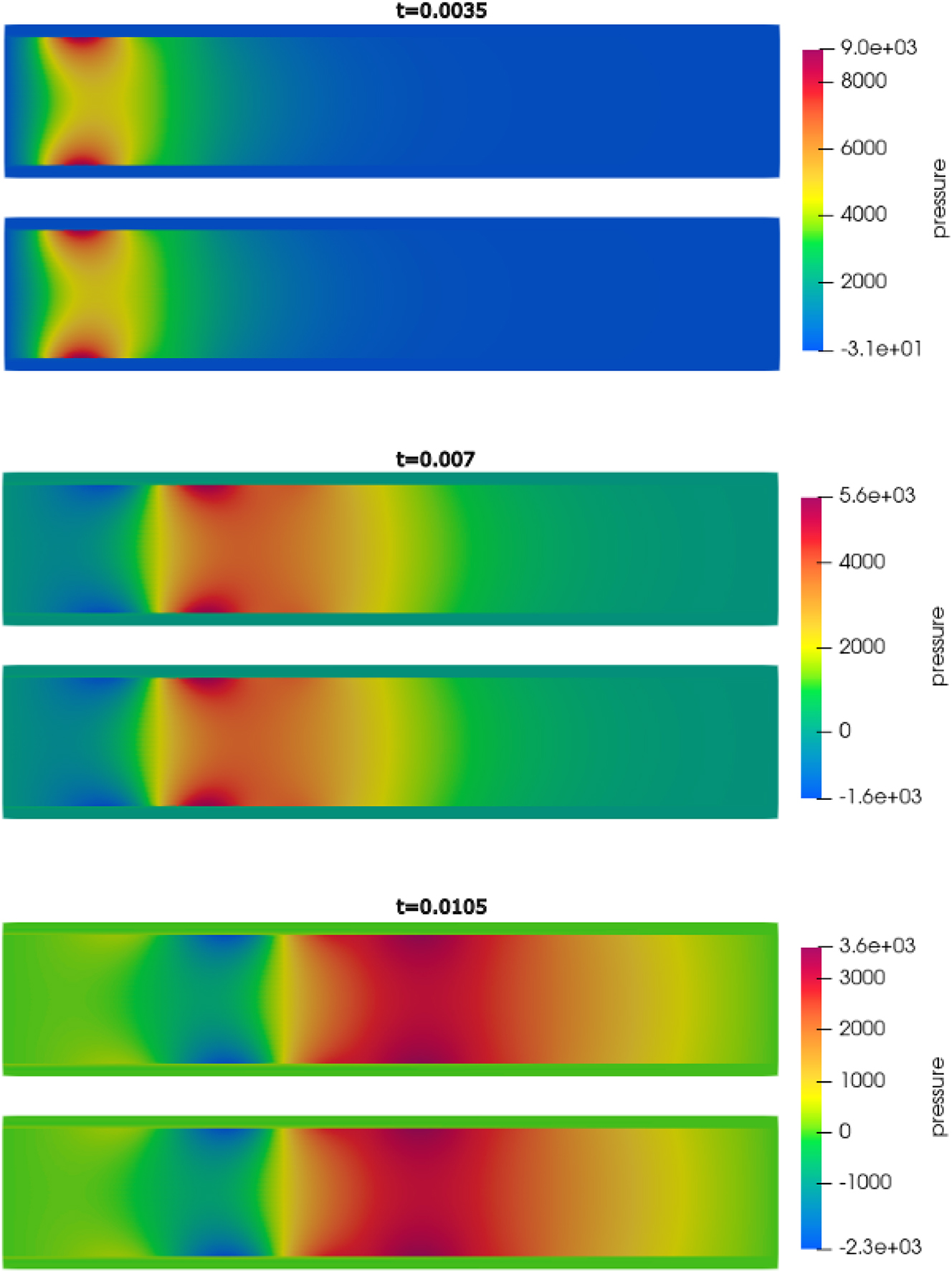
Example 2: Pressure surface plots for both Nitsche’s method (top) and our method (bottom) obtained with ϑ = 1 at times t = 0.0035, 0.007, 0.0105 s. The domain has been reflected in ParaView to recover the full channel.

The average number of subiterations in Step 1 of our method is 5.08 when ϑ = 1 and 4.16 when ϑ = 1/2, which is less than most of the values in Table 1 for L = 1 000. Overall, this example demonstrates that our method is on par with the monolithic scheme based on Nitsche’s method when ϑ = 1, and that it can easily provide more accurate solution by taking ϑ = 1/2.

7 Conclusions

In this work, we present a partitioned, strongly-coupled method for the interaction between a fluid and a poroelastic structure. This method uses the Biot’s problem in the dual-mixed formulation, which is enabled by employing the Robin boundary conditions at the interface. The proposed method features second-order accuracy when ϑ = 1/2, in which case it has no numerical dissipation. We proved that the method is unconditionally stable provided ϑ ∈ [1/2, 1], and that the subiterative process in Step 1 of our algorithm is convergent.

We investigated the properties of the proposed method in numerical examples. In Example 1, we investigated the rates of convergence with respect to the combination parameter, L, used in the Robin boundary conditions and with respect to parameter ϑ. While for most of the L values we considered, optimal convergence was obtained, we noticed some loss of accuracy if L was too large. For a fixed value of L, we observed an increase in the error as ϑ was increased from 1/2 to 1, with an exception of ϑ = 1/2 + τ, which exhibited the smallest errors. The first order convergence was obtained for all ϑ values except ϑ = 1/2 and ϑ = 1/2 + τ, which gave second order convergence. We also examined the properties of the proposed method if no subiterations are used in Step 1. While no instabilities are observed in this case, the convergence rates appear to be quite sensitive with respect to L. In particular, we observe the second order convergence rates for the Darcy velocity when certain values of L are used even with ϑ = 1, but also suboptimal convergence rates for the structure displacement for some values of L and ϑ = 1/2. To understand the relation between the convergence rates and the parameter L, we need to carefully derive the rates of convergence for the loosely coupled scheme while tracking the problem parameters, which is the focus of our ongoing work.

Finally, we compared the solutions obtained using our method to the ones obtained using a monolithic scheme on a 2D example of a propagating pressure wave. Our results show near perfect alignment of our method with the monolithic scheme when the same discretization parameters are used.

Corresponding author: Martina Bukač, Department of Applied and Computational Mathematics and Statistics, University of Notre Dame, Notre Dame, IN 46556, USA, E-mail: mbukac@nd.edu

Funding source: National Science Foundation

Award Identifier / Grant number: 2208219

Award Identifier / Grant number: 2205695

Research Ethics: Not applicable.
Informed consent: Not applicable.
Author contributions: MB: conceptualization, methodology, supervision, writing. CP: analysis, implementation, computations, writing. All authors have accepted responsibility for the entire content of this manuscript and approved its submission.
Use of Large Language Models, AI and Machine Learning Tools: None declared.
Conflict of interest: The authors state no conflict of interest.
Research funding: This work has been supported in part by the National Science Foundation via grants NSF DMS-2208219 and NSF DMS-2205695.
Data availability: Data supporting the findings of this study are available upon request from the corresponding author.

References

[1] A. Goriely, et al.., “Mechanics of the brain: perspectives, challenges, and opportunities,” Biomech. Model. Mechanobiol., vol. 14, no. 5, pp. 931–965, 2015. https://doi.org/10.1007/s10237-015-0662-4.Search in Google Scholar PubMed PubMed Central

[2] C. McCutchen, “Cartilage is poroelastic, not viscoelastic (including and exact theorem about strain energy and viscous loss, and an order of magnitude relation for equilibration time),” Journal of Biomechanics, vol. 15, no. 4, pp. 325–327, 1982, https://doi.org/10.1016/0021-9290(82)90178-6.Search in Google Scholar PubMed

[3] V. M. Calo, N. F. Brasher, Y. Bazilevs, and T. J. R. Hughes, “Multiphysics model for blood flow and drug transport with application to patient-specific coronary artery flow,” Computational Mechanics, vol. 43, pp. 161–177, 2008, https://doi.org/10.1007/s00466-008-0321-z.Search in Google Scholar

[4] P. H. Feenstra and C. A. Taylor, “Drug transport in artery walls: a sequential porohyperelastic-transport approach,” Computer Methods in Biomechanics and Biomedical Engineering, vol. 12, no. 3, pp. 263–276, 2009, https://doi.org/10.1080/10255840802459396.Search in Google Scholar PubMed

[5] M. Bukač, I. Yotov, and P. Zunino, “Dimensional model reduction for flow through fractures in poroelastic media,” ESAIM: Mathematical Modelling and Numerical Analysis, vol. 51, no. 4, pp. 1429–1471, 2017.Search in Google Scholar

[6] I. Ambartsumyan, E. Khattatov, I. Yotov, and P. Zunino, “A Lagrange multiplier method for a Stokes–Biot fluid–poroelastic structure interaction model,” Numerische Mathematik, vol. 140, no. 2, pp. 513–553, 2018, https://doi.org/10.1007/s00211-018-0967-1.Search in Google Scholar

[7] M. Bukač, I. Yotov, R. Zakerzadeh, and P. Zunino, “Partitioning strategies for the interaction of a fluid with a poroelastic material based on a Nitsche’s coupling approach,” Computer Methods in Applied Mechanics and Engineering, vol. 292, pp. 138–170, 2015, https://doi.org/10.1016/j.cma.2014.10.047.Search in Google Scholar

[8] A. Seboldt, O. Oyekole, J. Tambaca, and M. Bukač, “Numerical modeling of the fluid–porohyperelastic structure interaction,” SIAM Journal on Scientific Computing, vol. 43, no. 4, pp. A2923–A2948, 2021, https://doi.org/10.1137/20m1386268.Search in Google Scholar

[9] O. Oyekole and M. Bukač, “Second-order, loosely coupled methods for fluid–poroelastic material interaction,” Numerical Methods for Partial Differential Equations, vol. 36, no. 4, pp. 800–822, 2020, https://doi.org/10.1002/num.22452.Search in Google Scholar

[10] R. Zakerzadeh and P. Zunino, “A computational framework for fluid–porous structure interaction with large structural deformation,” Meccanica, vol. 54, no. 1, pp. 101–121, 2019, https://doi.org/10.1007/s11012-018-00932-x.Search in Google Scholar

[11] W. M. Boon, D. Gläser, R. Helmig, K. Weishaupt, and I. Yotov, “A mortar method for the coupled Stokes–Darcy problem using the MAC scheme for Stokes and mixed finite elements for Darcy,” Computational Geosciences, vol. 28, pp. 1–18, 2024, https://doi.org/10.1007/s10596-023-10267-6.Search in Google Scholar

[12] Y. Cao, M. Gunzburger, F. Hua, and X. Wang, “Coupled Stokes–Darcy model with Beavers–Joseph interface boundary condition,” Communications in Mathematical Sciences, vol. 8, no. 1, pp. 1–25, 2010, https://doi.org/10.4310/cms.2010.v8.n1.a2.Search in Google Scholar

[13] M. A. Murad and J. H. Cushman, “Thermomechanical theories for swelling porous media with microstructure,” International Journal of Engineering Science, vol. 38, no. 5, pp. 517–564, 2000, https://doi.org/10.1016/s0020-7225(99)00054-3.Search in Google Scholar

[14] W. Layton, H. Tran, and X. Xiong, “Long time stability of four methods for splitting the evolutionary Stokes–Darcy problem into Stokes and Darcy subproblems,” J. Comput. Appl. Math., vol. 236, no. 13, pp. 3198–3217, 2012, https://doi.org/10.1016/j.cam.2012.02.019.Search in Google Scholar

[15] M. Kubacki and M. Moraiti, “Analysis of a second-order, unconditionally stable, partitioned method for the evolutionary Stokes–Darcy model,” Int. J. Numer. Anal. Model, vol. 12, no. 4, pp. 704–730, 2015.Search in Google Scholar

[16] V. Girault and B. Rivière, “DG approximation of coupled Navier–Stokes and Darcy equations by Beaver–Joseph–Saffman interface condition,” SIAM Journal on Numerical Analysis, vol. 47, no. 3, pp. 2052–2089, 2009, https://doi.org/10.1137/070686081.Search in Google Scholar

[17] T. Bodnár, G. P. Galdi, and Š. Nečasová, Fluid–Structure Interaction and Biomedical Applications, Heidelberg, Germany, Springer, 2014.Search in Google Scholar

[18] E. Burman, R. Durst, and J. Guzmán, “Stability and error analysis of a splitting method using Robin–Robin coupling applied to a fluid–structure interaction problem,” Numerical Methods for Partial Differential Equations, vol. 38, no. 5, pp. 1396–1406, 2022, https://doi.org/10.1002/num.22840.Search in Google Scholar

[19] G. Gigante and C. Vergara, “On the stability of a loosely-coupled scheme based on a Robin interface condition for fluid–structure interaction,” Computers & Mathematics with Applications, vol. 96, pp. 109–119, 2021, https://doi.org/10.1016/j.camwa.2021.05.012.Search in Google Scholar

[20] S. Badia, A. Quaini, and A. Quarteroni, “Coupling Biot and Navier–Stokes equations for modelling fluid–poroelastic media interaction,” J. Comput. Phys., vol. 228, no. 21, pp. 7986–8014, 2009, https://doi.org/10.1016/j.jcp.2009.07.019.Search in Google Scholar

[21] A. Cesmelioglu, “Analysis of the coupled Navier–Stokes/Biot problem,” Journal of Mathematical Analysis and Applications, vol. 456, no. 2, pp. 970–991, 2017, https://doi.org/10.1016/j.jmaa.2017.07.037.Search in Google Scholar

[22] R. E. Showalter, “Poroelastic filtration coupled to Stokes flow,” in Control Theory of Partial Differential Equations, Boca Raton, Florida, USA, Chapman and Hall/CRC, 2005, pp. 243–256.Search in Google Scholar

[23] P. Causin, J. F. Gerbeau, and F. Nobile, “Added-mass effect in the design of partitioned algorithms for fluid–structure problems,” Computer Methods in Applied Mechanics and Engineering, vol. 194, nos. 42–44, pp. 4506–4527, 2005, https://doi.org/10.1016/j.cma.2004.12.005.Search in Google Scholar

[24] C. Förster, W. Wall, and E. Ramm, “Artificial added mass instabilities in sequential staggered coupling of nonlinear structures and incompressible viscous flows,” Computer Methods in Applied Mechanics and Engineering, vol. 196, no. 7, pp. 1278–1293, 2007, https://doi.org/10.1016/j.cma.2006.09.002.Search in Google Scholar

[25] F. Brezzi and M. Fortin, Mixed and Hybrid Finite Element Methods, vol. 15, New York, USA, Springer Science & Business Media, 2012.Search in Google Scholar

[26] A. Masud and T. J. Hughes, “A stabilized mixed finite element method for Darcy flow,” Computer Methods in Applied Mechanics and Engineering, vol. 191, nos. 39–40, pp. 4341–4370, 2002, https://doi.org/10.1016/s0045-7825(02)00371-7.Search in Google Scholar

[27] T. Li and I. Yotov, “A mixed elasticity formulation for fluid–poroelastic structure interaction,” ESAIM: Mathematical Modelling and Numerical Analysis, vol. 56, no. 1, pp. 1–40, 2022, https://doi.org/10.1051/m2an/2021083.Search in Google Scholar

[28] N. Koshiba, J. Ando, X. Chen, and T. Hisada, “Multiphysics simulation of blood flow and ldl transport in a porohyperelastic arterial wall model,” Journal of Biomedical Engineering, vol. 129, pp. 374–385, 2007. https://doi.org/10.1115/1.2720914.Search in Google Scholar PubMed

[29] J. Wen, J. Su, Y. He, and H. Chen, “Discontinuous galerkin method for the coupled Stokes–Biot model,” Numerical Methods for Partial Differential Equations, vol. 37, no. 1, pp. 383–405, 2021, https://doi.org/10.1002/num.22532.Search in Google Scholar

[30] X. Wang and H. Rui, “A semi-decoupled MAC scheme for the coupled fluid–poroelastic material interaction,” Computers & Mathematics with Applications, vol. 139, pp. 118–135, 2023, https://doi.org/10.1016/j.camwa.2023.04.003.Search in Google Scholar

[31] H. Kunwar, H. Lee, and K. Seelman, “Second-order time discretization for a coupled quasi-Newtonian fluid–poroelastic system,” International Journal for Numerical Methods in Fluids, vol. 92, no. 7, pp. 687–702, 2020, https://doi.org/10.1002/fld.4801.Search in Google Scholar

[32] M. Bukač, A. Seboldt, and C. Trenchea, “Refactorization of Cauchy’s method: a second-order partitioned method for fluid–thick structure interaction problems,” Journal of Mathematical Fluid Mechanics, vol. 23, no. 3, p. 64, 2021, https://doi.org/10.1007/s00021-021-00593-z.Search in Google Scholar

[33] J. Burkardt and C. Trenchea, “Refactorization of the midpoint rule,” Applied Mathematics Letters, vol. 107, p. 106438, 2020, https://doi.org/10.1016/j.aml.2020.106438.Search in Google Scholar

[34] G. Avalos, E. Gurvich, and J. T. Webster, “Weak and strong solutions for a fluid-poroelastic-structure interaction via a semigroup approach,” Applied Mathematics Letters, vol. 107, p. 106438, 2024.Search in Google Scholar

[35] V. Girault and P.-A. Raviart, Finite Element Approximation of the Navier–Stokes Equations, vol. 749, Berlin, Springer, 1979.Search in Google Scholar

[36] M. Bukač, G. Fu, A. Seboldt, and C. Trenchea, “Time-adaptive partitioned method for fluid–structure interaction problems with thick structures,” J. Comput. Phys., vol. 473, p. 111708, 2023, https://doi.org/10.1016/j.jcp.2022.111708.Search in Google Scholar

[37] F. Hecht, “New development in FreeFem++,” Journal of Numerical Mathematics, vol. 20, nos. 3–4, pp. 251–265, 2012, https://doi.org/10.1515/jnum-2012-0013.Search in Google Scholar

[38] M. Bukač, S. Čanić, R. Glowinski, J. Tambača, and A. Quaini, “Fluid–structure interaction in blood flow capturing non-zero longitudinal structure displacement,” J. Comput. Phys., vol. 235, pp. 515–541, 2013, https://doi.org/10.1016/j.jcp.2012.08.033.Search in Google Scholar

[39] M. Bukač and C. Trenchea, “Adaptive, second-order, unconditionally stable partitioned method for fluid–structure interaction,” Computer Methods in Applied Mechanics and Engineering, vol. 393, p. 114847, 2022, https://doi.org/10.1016/j.cma.2022.114847.Search in Google Scholar

[40] X. Ma, G. Lee, and S. Wu, “Numerical simulation for the propagation of nonlinear pulsatile waves in arteries,” Journal of Biomechanical Engineering, vol. 114, no. 4, pp. 490–496, 1992. https://doi.org/10.1115/1.2894099.Search in Google Scholar PubMed

Received: 2024-04-25

Accepted: 2024-11-04

Published Online: 2025-02-24

Published in Print: 2025-09-25

This work is licensed under the Creative Commons Attribution 4.0 International License.

Articles in the same Issue

https://doi.org/10.1515/jnma-2024-0057

Keywords for this article

fluid–poroelastic structure interaction; partitioned method; second-order; strongly coupled; mixed formulation

Creative Commons

BY 4.0