A subspace framework for L ∞ model reduction
-
Emre Mengi


Abstract
We propose an approach for the
1 Introduction
Various applications give rise to linear time-invariant (LTI) descriptor systems; see, e.g., [1], [2], [3], [4], and references therein. A model order reduction problem for such a system typically concerns the approximation of the system with a system of smaller and prescribed order. Here we deal with one of them, namely the
We assume that the LTI descriptor system under consideration is available in a state-space representation
for given matrices
with the
where σ
max(⋅) denotes the largest singular value of its matrix argument, and the last equality holds as A, B, C, D, E are real matrices. Note that we customarily set
which in turn is equal to the induced norm of the operator φ: L 2 → L 2 associated with (1) in the time domain mapping u to y as φu = y (for an explicit expression for φ see Ref. [3], Theorem 2.29]), that is given by
Hence, under the asymptotic stability assumption on the descriptor system in (1), we have
The
described by the matrices
Furthermore, let S = (A, E, B, C, D) be the given system of order n and with the transfer function H as in (2). Setting
over all descriptor systems
Two important remarks are in order regarding the minimization of the objective in (5). First, in addition to non-convexity, an additional difficulty is the nonsmooth nature of the problem. The objective in (5) as a function of
where
1.1 Literature and contributions
For an asymptotically stable descriptor system with the transfer function H, the H
∞ model reduction problem – that is, for a given small order
A classical alternative is finding a best approximation with respect to the Hankel norm (HNA) [12] rather than the
The iterative rational Krylov algorithm (IRKA) [15] was introduced in order to find a reduced system of prescribed order that is locally optimal with respect to the
Here, we propose an approach to compute a local minimizer of
Smooth optimization techniques have been recently used for model order reduction of asymptotically stable structured systems [26]. It is also observed over there that a direct minimization of the
On a related note, our recent work [28] concerns the minimization of the
1.2 Outline
We first consider the direct minimization of
2 Use of first-order and second-order derivative-based methods
First-order methods such as the gradient descent algorithm, and second-order methods such as quasi-Newton algorithms equipped with proper line-searches have been successfully applied to nonsmooth optimization problems in recent years [22], [23], [31], [32]. In these circumstances, if a curvature condition is employed in the line-search, this should take into consideration that the directional derivatives need not converge to zero unlike the situation for smooth optimization problems, e.g., if Wolfe conditions are imposed in the line-search, weak Wolfe conditions should be used rather than strong Wolfe conditions [23], Section 4]. Also, for termination small gradient norms should not be required. Instead, for instance, a failure to take a reasonably long step in the objective along the descent search direction may indicate convergence to a locally optimal solution [31], Section 3].
The objective to be minimized in (5) for the
where
The gradient descent algorithm, as well as quasi-Newton algorithms to minimize
ensuring that
where Re(⋅), Im(⋅) denote the real part, imaginary part, respectively, of their vector or matrix arguments. Also, above ⊙ denotes the Hadamard product,
It is essential that a quasi-Newton method such as BFGS generates approximate Hessians that are positive definite. This is traditionally imposed by the line-searches. For instance, if BFGS is to be used to minimize
One difficulty with using methods such as gradient descent and BFGS to minimize
To illustrate the slow convergence issues described in the previous paragraph, and the computational difficulties that come with it, we apply the gradient descent algorithm to the iss example from the SLICOT collection. The system associated with this example has order n = 270, and m = p = 3. We attempt to solve the
This concerns the iss example with
| k |
|
|
|---|---|---|
| 0 | 0.004470060020 | 1.000093488 |
| 1 | 0.004346739384 | 0.833556647 |
| 2 | 0.003609940202 | 1.000097230 |
| 3 | 0.003175718111 | 0.769359926 |
| 4 | 0.002975716755 | 1.000095596 |
| 5 | 0.002946113130 | 0.999918608 |
| 6 | 0.002697635041 | 0.844275929 |
| 7 | 0.002656707905 | 0.999952423 |
| 30 | 0.002415516341 | 0.803721909 |
| 31 | 0.002415479783 | 1.000008471 |
| 32 | 0.002415475189 | 0.803718441 |
| 33 | 0.002415456030 | 1.000008467 |
| 34 | 0.002415454613 | 0.803716708 |
| 35 | 0.002415444154 | 1.000008465 |
| 36 | 0.002415439844 | 0.803714645 |
| 37 | 0.002415438945 | 1.000008462 |
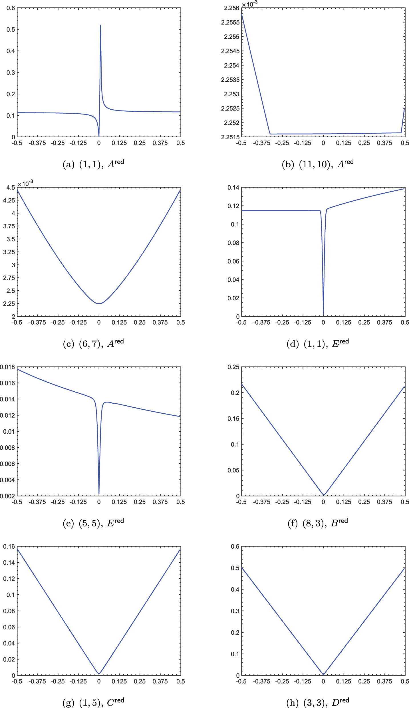
![Figure 1:
The locally minimal reduced system generated by the gradient descent method for the iss example and
r
=
12
$\mathsf{r}=12$
is varied, and the error
F
$\mathcal{F}$
is plotted as a function of the variation. In each one of the plots (a)–(h), only the indicated entry of one of the optimal coefficients
A
r
e
d
,
B
r
e
d
,
C
r
e
d
,
D
r
e
d
,
E
r
e
d
${A}^{\mathsf{r}\mathsf{e}\mathsf{d}},{B}^{\mathsf{r}\mathsf{e}\mathsf{d}},{C}^{\mathsf{r}\mathsf{e}\mathsf{d}},{D}^{\mathsf{r}\mathsf{e}\mathsf{d}},{E}^{\mathsf{r}\mathsf{e}\mathsf{d}}$
is varied by amounts in [−0.5, 0.5]. Zero variation corresponds to the optimal reduced system.](/document/doi/10.1515/jnma-2023-0115/asset/graphic/j_jnma-2023-0115_fig_001.jpg)
The locally minimal reduced system generated by the gradient descent method for the iss example and
3 A subspace framework
The computational difficulty in minimizing the objective
and solve the resulting
where
The question that we need to address is how do we form a small system S
q
= (A
q
, E
q
, B
q
, C
q
, D) that is a good representative of the original system near a local minimizer of the original
Recall how pure Newton’s method operates to minimize a function
To obtain the small system in (8), we employ projection-based model reduction. In particular, let
giving rise to a system of the form (8) with
For the realization of the ideas in the previous paragraph, we need to be equipped with a tool that gives us the capability to interpolate H(s) and its derivatives at a prescribed point in the complex plane with those of the transfer function for the small system. This tool is introduced in the next result, which follows from [35], Theorem 1].
Theorem 1.
Let
Then, with A q , E q , B q , C q defined as in (10), if A q − μE q is invertible, we have
H(μ) = H q (μ) and
Our proposed subspace framework at iteration r first finds a minimizer of
Computing such an ω
q
requires the large-scale
Algorithm 1
(subspace framework for
|
Input:
System S = (A, E, B, C, D) as in (1), the order
|
|
Output:
Estimate
|
|
1: Choose the initial subspaces
|
| 2: Form A 0, B 0, C 0, E 0 using (10), and let S 0 = (A 0, E 0, B 0, C 0, D). |
| % main loop |
| 3: for q = 0, 1, … do |
| 4: if q ⩾ 1 then |
|
5:
|
| 6: end if |
|
7: ω
q
← a maximizer of
|
|
8:
if
q
|
|
9:
Return
if convergence has occurred with
|
| 10: end if |
| % expand the subspaces to interpolate at iω q |
|
11:
|
|
12:
|
|
13:
|
| % update the small system |
| 14: Form A q+1, B q+1, C q+1, E q+1 using (10), and let S q+1 = (A q+1, E q+1, B q+1, C q+1, D). |
| % refine the small system |
| 15: Refine V q+1, W q+1 and S q+1 if necessary (using Algorithm 2 below in Section 3.1). |
| 16: end for |
3.1 Refinement step
First we make a few observations regarding the relation between
At the qth iteration of Algorithm 1 right after line 14, by Theorem 1, we have
for j = 1, 2, 3 under the assumptions that A − iω
q
E and A
q+1 − iω
q
E
q+1 are invertible. Consequently,
and recalling
Indeed, as the singular values and vectors of
for j = 1, 2. Now ω
q
is a global maximizer of
Assuming that the last inequality on the second derivative above holds strictly, (14) implies ω
q
is also a local maximizer of
Regarding
where the third equality is due to the interpolatory property in (13). As argued in the previous paragraph, the point ω
q
is not only a global maximizer of
In the refinement step, if it happens that ω
q
is merely a local maximizer of
Assuming
Algorithm 2
(refinement step).
| 1: for j = 0, 1, … do |
|
2:
|
|
3:
if
|
| 4: Terminate with V q+1, W q+1 and S q+1. |
| 5: end if |
|
%
expand the subspaces to interpolate at
|
|
6:
|
|
7:
|
|
8:
|
| % update the small system |
| 9: Form A q+1, B q+1, C q+1, E q+1 using (10), |
| and let S q+1 = (A q+1, E q+1, B q+1, C q+1, D). |
| 10: end for |
4 Interpolation properties of the subspace framework
Suppose that ω
q
is a global maximizer of
and by employing (11), it is apparent that
for all y, z ∈ {ω, x 1, x 2}. By exploiting
and using implicit differentiation
for y ∈ {x
1, x
2}, where the second equality is due to (18), as well as (17) implying the fact that
Moreover, for any y, z ∈ {ω, x 1, x 2}, we have
due to (18) and (19) combined with the fact that
for any y, z ∈ {x 1, x 2}.
5 A quadratic convergence result regarding Algorithm 1
In this section, we establish quadratic convergence of the iterates of Algorithm 1 under additional smoothness assumptions. Here and in the next section,
where vec(M) denotes the vector obtained by stacking up the columns of matrix M. The gradients
We assume that there are two consecutive iterates
Assumption 2.
The maximum of
An assumption regarding the smoothness of
Assumption 3.
For every
the maximum of
the singular value
Moreover, all of the third derivatives of
We state and prove the main result that relates
Theorem 4.
Suppose that two consecutive iterates
Proof.
By continuity
By an application of Taylor’s theorem with integral remainder, we have
where, for the third equality, we have used the Lipschitz continuity of
where the third equality is due to
By employing (24) in (23), we deduce
Finally, noting
as desired. □
6 Dealing with asymptotic stability constraints
In many applications, in addition to the objective that the reduced-order system sought
In this setting, with
for a prescribed negative real number β, where
Extension of the proposed subspace framework, that is Algorithm 1, to deal with the constrained minimization problem in (25) rather than the unconstrained minimization of
for the reduced function
where Re(z) denotes the real part of a complex scalar
We remark that, assuming ω
q
is again a global maximizer of
still hold. Moreover, if a logarithmic barrier approach is adopted for the solution of the constrained problems, then, in essence, constrained problems are turned into unconstrained problems by lifting the constraints to the objective via the logarithmic barrier functions
associated with problems (25), (26), respectively, where log(⋅) denotes the natural logarithm of its parameter, μ is a positive real number and represent the barrier parameter. In this case, the interpolation properties extend to the logarithmic barrier functions as well. In particular, we have
for every positive real number μ.
There are alternatives to our approach above to enforce asymptotic stability on the reduced system. One possibility is to define the
7 Practical issues
Here we spell out a few practical issues regarding Algorithm 1 such as how we form the initial systems S
0,
7.1 Initialization
The initial subspaces
where Im(s
k
) denotes the imaginary part of
for j = 1, 2, 3 and k = 1, …, ℓ.
Additionally, at every subspace iteration with q > 0, an initial point is needed for the solution of the minimization problem in line 5 of Algorithm 1 regardless of how it is solved, e.g., via gradient descent or BFGS. This initialization carries significance, as it affects which local minimizer of
the model of order
the model of order
An issue that requires attention is that
for a diagonal matrix Λ and invertible U at ease. We also have the eigenvalue decomposition
at hand. Note that the middle factors in eigenvalue decompositions above are the same, as T
2 has the same eigenvalues as the pencil
Hence, we can use
as the matrices of the initial system
Remark 1.
The invertibility assumption above on
Remark 2.
When the pencil
To see VU
−1 is real for particular choices of T
2, U, suppose a ± ib consist of a pair of complex conjugate eigenvalues of
so the real matrix on the left has the eigenvalues a ± ib, and we use it on the 2×2 diagonal block of T
2 with row and column indices ℓ, ℓ + 1. Using the decomposition in (28), in particular Z
−1, we can set up U so that
7.2 Termination
The termination in line 9 of Algorithm 1 is determined based on the values of
To be precise, we terminate at the qth subspace iteration in line 9 if q ≥ 1 and
for a prescribed tolerance
The termination condition for the minimizer to solve the minimization problem in line 5 of Algorithm 1 also requires some care. Recall that the objective
As for the termination condition of the refinement step (i.e., the condition in line 3 of Algorithm 2) employed in practice, we rely on
where we again use the same tolerance
7.3 Orthonormalization of the bases for the subspaces
Keeping the bases for the subspaces
This orthonormality property of the bases is attained in line 13 of Algorithm 1, as well as line 8 of Algorithm 2. In line 13 of Algorithm 1, V
q
and W
q
are already orthonormal bases for
Near convergence the interpolation points iω
q
of Algorithm 1 start not changing by much in consecutive iterations. This results in the new expansion directions
7.4 Solution of the reduced
L
∞
-norm minimization problem
We use BFGS to minimize the reduced
7.5 Computation of the
L
∞
norm
Algorithm 1 in line 7 requires the computation of the
8 Numerical results
In this section, we report the results of numerical experiments performed with a MATLAB implementation of Algorithm 1 taking also the practical issues indicated in the previous section into account. Sections 8.1 and 8.2 concern experiments on rather smaller order systems, Section 8.3 concerns experiments on a system of medium order, while the results of experiments on several large-order systems are reported in Section 8.4. All of the experiments are conducted in MATLAB 2020b on an iMac with Mac OS 12.1 operating system, Intel® Core™ i5-9600K CPU and 32GB RAM.
The numerical experiments are performed using the variation of the MATLAB implementation of BFGS due to Michael L. Overton for the solution of the reduced
For comparison or initialization purposes, some of the numerical experiments involve the application of balanced truncation for which we use the MATLAB toolbox MORLAB-5.0 [47], in particular the routine ml_ct_dss_bt or ml_ct_ss_bt depending on whether the system at hand is a descriptor system or more specifically a linear time-invariant system. Moreover, the Hankel singular values computed for smaller systems for comparison purposes are retrieved by calling the built-in routine hankelsv in MATLAB. As the first three subsections concern the model reduction of relatively smaller systems, the built-in routine norm is employed in line 7 of Algorithm 1 for
8.1 ISS example
We start with the iss example of order n = 270 that is also considered when optimizing the objective
The figure is similar to Figure 1 and concerns the iss example with
The largest singular values of the errors
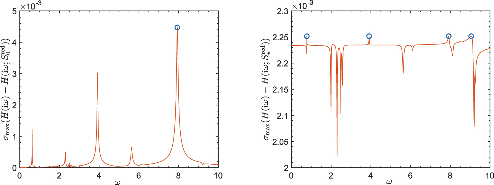
The plots of
Information about the progress of Algorithm 1 is given in Table 2. We start with the reduced system S
0 of order 36 that interpolates the original system S of order 270 at three points on the imaginary axis, namely the imaginary parts of the most dominant three poles of S with NIPs. At every iteration, if no refinement step is performed, the order of the reduced system S
q
increases by 4m = 12. Additionally, each refinement step results in an increase of 4m = 12 in the order of S
q
. We observe in the second column that the error
The iterates and information about the progress of Algorithm 1 on the iss example with
| q |
|
Red order | # BFGS iter | # fun evals | # refine |
|---|---|---|---|---|---|
| 0 | 0.004470060020 | 36 | — | — | 2 |
| 1 | 0.003517059977 | 72 | 38 | 105 | 0 |
| 2 | 0.002259657400 | 84 | 45 | 155 | 2 |
| 3 | 0.002252138011 | 120 | 35 | 123 | 0 |
| 4 | 0.002251613679 | 132 | 11 | 48 | 0 |
| 5 | 0.002251609387 | 144 | 2 | 29 | 0 |
| 6 | 0.002251607779 | 156 | 2 | 32 | — |
8.2 CD player model
Our next example is the CD player model which is available in the SLICOT library. The model is a linear-time invariant system of order n = 120 and with m = 2 inputs and p = 2 outputs. The details of the model can be found in Ref. [48], and the references therein. Our primary purpose here is to compare on this example Algorithm 1 with the approach in Ref. [16] for
The reduced systems
This table concerns the “CD player model”. Relative errors
|
|
Alg. 1 | IHA | MBT | HNA | BT | Lower Bnd |
|---|---|---|---|---|---|---|
| 2 | 3.12 × 10⁻¹ | 3.66 × 10⁻¹ | 3.68 × 10⁻¹ | 3.35 × 10⁻¹ | 3.69 × 10⁻¹ | 1.95 × 10⁻¹ |
| 4 | 1.82 × 10⁻² | 2.14 × 10⁻² | 2.25 × 10⁻² | 2.00 × 10⁻² | 2.25 × 10⁻² | 1.13 × 10⁻² |
| 6 | 9.44 × 10⁻³ | 1.04 × 10⁻² | 1.19 × 10⁻² | 1.23 × 10⁻² | 1.23 × 10⁻² | 6.79 × 10⁻³ |
| 8 | 4.18 × 10⁻³ | 4.85 × 10⁻³ | 6.40 × 10⁻³ | 5.99 × 10⁻³ | 6.41 × 10⁻³ | 3.20 × 10⁻³ |
| 10 | 7.45 × 10⁻⁴ | 8.99 × 10⁻⁴ | 1.24 × 10⁻³ | 1.08 × 10⁻³ | 1.32 × 10⁻³ | 5.86 × 10⁻⁴ |
We give some details of Algorithm 1 applied to find a reduced system of order
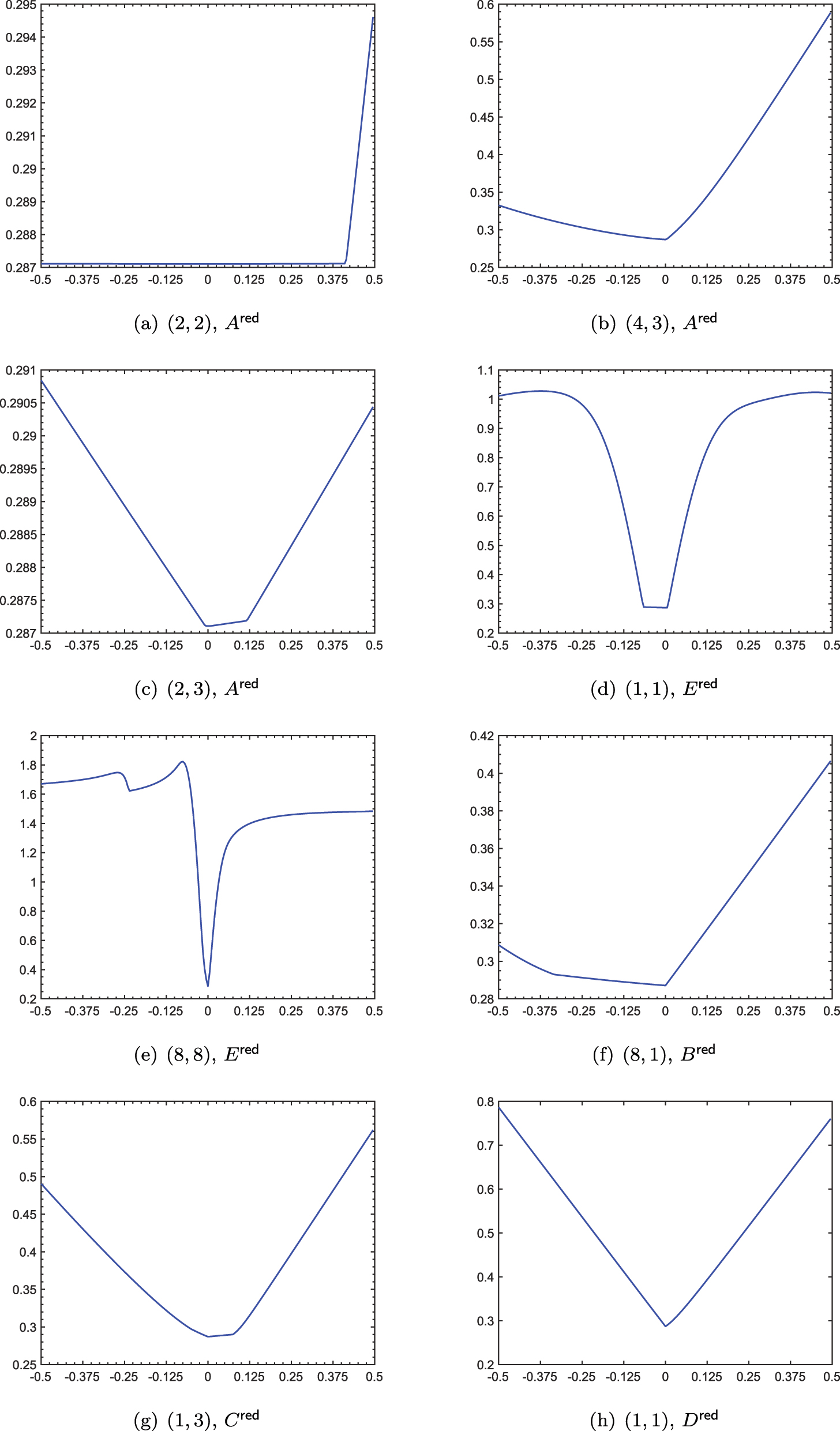
The figure is analogous to Figure 1, but concerns the “CD player model” with
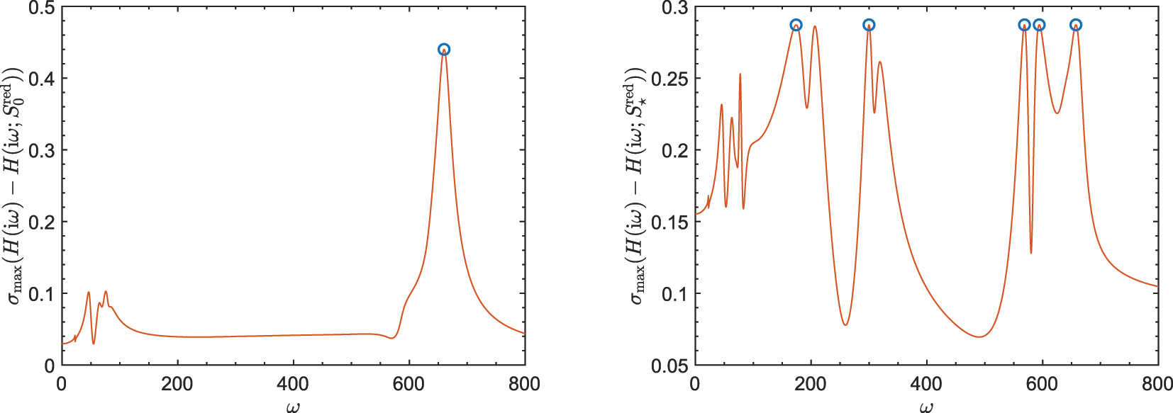
The plots illustrate the errors of the initial, optimal models by Algorithm 1 for the “CD player model” with
The iterates and information about the progress of Algorithm 1 on the “CD player model” for finding a reduced system or order
| q |
|
Red order | # BFGS iter | # fun evals | # refine |
|---|---|---|---|---|---|
| 0 | 0.439972058849 | 12 | — | — | 1 |
| 1 | 0.291281639337 | 20 | 565 | 1,479 | 0 |
| 2 | 0.287107598817 | 24 | 134 | 387 | 0 |
| 3 | 0.287107598817 | 28 | 1 | 32 | — |
8.3 FOM model
We next report numerical results on the FOM example available in the SLICOT library. The FOM example is a linear time-invariant system of order n = 1,006, and with m = p = 1. The details are given in Ref. [49], Example 3]. Here, we are mainly interested in investigating the quality of the estimates for optimal reduced systems produced by Algorithm 1. To this end, we compare the errors of the reduced systems by Algorithm 1 with those of balanced truncation, as well as the theoretical lower bounds for the errors in terms of Hankel singular values for varying choices of prescribed order
In Figure 6, the
![Figure 6:
Errors of the reduced systems of order
r
∈
[
2,11
]
$\mathsf{r}\in \left[2,11\right]$
produced by Algorithm 1 and balanced truncation (BT), as well as the
(
r
+
1
)
$\left(\mathsf{r}+1\right)$
st largest Hankel singular value
σ
r
+
1
${\sigma }_{\mathsf{r}+1}$
for the FOM example.](/document/doi/10.1515/jnma-2023-0115/asset/graphic/j_jnma-2023-0115_fig_006.jpg)
Errors of the reduced systems of order
8.4 Systems with large order
Finally, we report results on systems with large order arising from modeling of power plants due to Rommes and his colleagues. All of these large-scale examples are available on the website of Rommes.[1]
Unlike the previous three subsections, we form the initial estimate for the minimizer
Even Algorithm 1 requires the computation of the
The absolute and relative errors of the computed reduced systems of order
The absolute errors
| Example | n, m = p |
|
Approach | Error | Rel error | Time |
|---|---|---|---|---|---|---|
| S20PI_n | 1,182, 1 | 12 | Alg. 1 | 7.67 × 10⁻¹ | 2.23 × 10⁻¹ | 19.8 |
| S20PI_n | 1,182, 1 | 16 | Alg. 1 | 7.66 × 10⁻¹ | 2.22 × 10⁻¹ | 36.2 |
| S20PI_n | 1,182, 1 | 12 | BT | 1.76 × 100 | 5.11 × 10⁻¹ | — |
| S20PI_n | 1,182, 1 | 16 | BT | 1.32 × 100 | 3.84 × 10⁻¹ | — |
| S40PI_n | 2,182, 1 | 12 | Alg. 1 | 9.30 × 10⁻¹ | 2.78 × 10⁻¹ | 48.1 |
| S40PI_n | 2,182, 1 | 16 | Alg. 1 | 6.71 × 10⁻¹ | 2.00 × 10⁻¹ | 38.1 |
| S40PI_n | 2,182, 1 | 32 | BT | 1.75 × 100 | 5.23 × 10⁻¹ | — |
| M40PI_n | 2,182, 3 | 12 | Alg. 1 | 1.99 × 100 | 5.22 × 10⁻¹ | 52.2 |
| M40PI_n | 2,182, 3 | 24 | Alg. 1 | 1.70 × 100 | 4.45 × 10⁻¹ | 117.1 |
| M40PI_n | 2,182, 3 | 36 | BT | 3.07 × 100 | 8.03 × 10⁻¹ | — |
| ww_vref_6405 | 13,251, 1 | 12 | Alg. 1 | 5.80 × 10⁻⁴ | 2.04 × 10⁻¹ | 9.2 |
| ww_vref_6405 | 13,251, 1 | 16 | Alg. 1 | 4.19 × 10⁻⁴ | 1.48 × 10⁻¹ | 15.1 |
| xingo_afonso | 13,250, 1 | 12 | Alg. 1 | 3.55 × 10⁻² | 8.74 × 10⁻³ | 14.4 |
| xingo_afonso | 13,250, 1 | 16 | Alg. 1 | 3.56 × 10⁻² | 8.77 × 10⁻³ | 14.0 |
| xingo_afonso | 13,250, 1 | 20 | Alg. 1 | 1.13 × 10⁻² | 2.79 × 10⁻³ | 26.2 |
| bips07_1998 | 15,066, 4 | 16 | Alg. 1 | 1.24 × 101 | 6.30 × 10⁻² | 127.6 |
| bips07_1998 | 15,066, 4 | 32 | Alg. 1 | 9.67 × 100 | 4.91 × 10⁻² | 219.8 |
| bips07_3078 | 21,228, 4 | 16 | Alg. 1 | 1.27 × 101 | 6.06 × 10⁻² | 200.8 |
| bips07_3078 | 21,228, 4 | 32 | Alg. 1 | 1.00 × 101 | 4.78 × 10⁻² | 274.1 |
9 Software
A MATLAB implementation of Algorithm 1 is publicly available at https://zenodo.org/record/8344591. The numerical results reported in the previous section are obtained with this implementation. Scripts are included to reproduce the results for the CD player model in Section 8.2, and the xingo_afonso, bips07_1998 examples in Section 8.4. The results for other benchmark examples can be obtained similarly.
10 Conclusions
We have proposed an approach to find a locally optimal solution of the
The quality of the converged locally optimal solution depends on the initial guess for the optimal reduced system. To generate the initial guess, we have employed two different strategies based on balanced truncation and dominant poles. The first of these strategies may not be applicable unless the original system is asymptotically stable. On the other hand, there is no asymptotic stability requirement for the second strategy. However, a strategy generating a good initial guess is certainly worth further research. The proposed approach typically requires a few large-scale
Acknowledgment
The author is grateful to two anonymous referees for their invaluable feedback on the initial version of this manuscript.
-
Research ethics: Not applicable.
-
Informed consent: Not applicable.
-
Author contributions: The author has accepted responsibility for the entire content of this manuscript and approved its submission.
-
Use of Large Language Models, AI and Machine Learning Tools: None declared.
-
Conflict of interest: The authors state no conflict of interest.
-
Research funding: None declared.
-
Data availability: The raw data and codes associated with the current study are publicly available at https://zenodo.org/record/8344591 and https://sites.google.com/site/rommes/software.
References
[1] K. E. Brenan, S. L. Campbell, and L. R. Petzold, Numerical Solution of Initial-Value Problems in Differential-Algebraic Equations, 2nd ed. Philadelphia, PA, SIAM, 1996.10.1137/1.9781611971224Search in Google Scholar
[2] Y. Feng and M. Yagoubi, Robust Control of Linear Descriptor Systems, Singapore, Springer, 2017.10.1007/978-981-10-3677-4Search in Google Scholar
[3] P. Kunkel and V. Mehrmann, Differential-Algebraic Equations: Analysis and Numerical Solution, Zurich, Switzerland, EMS Press, 2006.10.4171/017Search in Google Scholar
[4] R. Riaza, Differential Algebraic Systems. Analytical Aspects and Circuit Applications. Notes on Mathematics and its Applications, Singapore, World Scientific, 2008.10.1142/9789812791818Search in Google Scholar
[5] A. C. Antoulas, Approximation of Large-Scale Dynamical Systems, Volume 6 of Adv. Des. Control, Philadelphia, PA, SIAM Publications, 2005.10.1137/1.9780898718713Search in Google Scholar
[6] V. Mehrmann and T. Stykel, “Balanced truncation model reduction for large-scale systems in descriptor form,” in Dimension Reduction of Large-Scale Systems, P. Benner, D. C. Sorensen, and V. Mehrmann, Eds., Berlin, Springer, vol. 45, 2005, pp. 83–115.10.1007/3-540-27909-1_3Search in Google Scholar
[7] B. Moore, “Principal component analysis in linear systems: controllability, observability, and model reduction,” IEEE Trans. Autom. Control, vol. 26, no. 1, pp. 17–32, 1981. https://doi.org/10.1109/tac.1981.1102568.Search in Google Scholar
[8] T. Stykel, “Gramian-based model reduction for descriptor systems,” Math. Contol Signals Syst., vol. 16, no. 4, pp. 297–319, 2004. https://doi.org/10.1007/s00498-004-0141-4.Search in Google Scholar
[9] S. Gugercin and A. C. Antoulas, “A survey of model reduction by balanced truncation and some new results,” Int. J. Control, vol. 77, no. 8, pp. 748–766, 2004. https://doi.org/10.1080/00207170410001713448.Search in Google Scholar
[10] S. Gugercin, D. C. Sorensen, and A. C. Antoulas, “A modified low-rank Smith method for large-scale Lyapunov equations,” Numer. Algorithm., vol. 32, no. 1, pp. 27–55, 2003. https://doi.org/10.1023/a:1022205420182.10.1023/A:1022205420182Search in Google Scholar
[11] T. Penzl, “A cyclic low-rank Smith method for large sparse Lyapunov equations,” SIAM J. Sci. Comput., vol. 21, no. 4, pp. 1401–1418, 1999. https://doi.org/10.1137/s1064827598347666.Search in Google Scholar
[12] K. Glover, “All optimal hankel-norm approximations of linear multivariable systems and their L∞${\mathcal{L}}_{\infty }$-error bounds,” Int. J. Control, vol. 39, no. 6, pp. 1115–1193, 1984. https://doi.org/10.1080/00207178408933239.Search in Google Scholar
[13] P. Benner and S. W. R. Werner, “Hankel-norm approximation of large-scale descriptor systems,” Adv. Comput. Math., vol. 46, Art.no. 40, 2020, https://doi.org/10.1007/s10444-020-09750-w.Search in Google Scholar
[14] P. Benner, E. S. Quintana-Orti, and G. Quintana-Orti, “Computing optimal hankel norm approximations of large-scale systems,” in Proceedings of 43rd IEEE Conference on Decision and Control, vol. 3, 2004, pp. 3078–3083.10.1109/CDC.2004.1428939Search in Google Scholar
[15] S. Gugercin, A. C. Antoulas, and C. Beattie, “
[16] G. Flagg, C. A. Beattie, and S. Gugercin, “Interpolatory H∞ model reduction,” Syst. Control Lett., vol. 62, no. 7, pp. 567–574, 2013. https://doi.org/10.1016/j.sysconle.2013.03.006.Search in Google Scholar
[17] C. K. Krzysztof, Methods of Descent for Nondifferentiable Optimization, Berlin, New York, Springer-Verlag, 1985.Search in Google Scholar
[18] M. M. Mäkelä and P. Neittaanmäki, Nonsmooth Optimization: Analysis and Algorithms with Applications to Optimal Control, Singapore, World Scientific, 1992.10.1142/1493Search in Google Scholar
[19] J. V. Burke, A. S. Lewis, and M. L. Overton, “Two numerical methods for optimizing matrix stability,” Linear Algebra Appl., vols. 351–352, pp. 117–145, 2002, https://doi.org/10.1016/s0024-3795(02)00260-4.Search in Google Scholar
[20] J. V. Burke, A. S. Lewis, and M. L. Overton, “A robust gradient sampling algorithm for nonsmooth, nonconvex optimization,” SIAM J. Opt., vol. 15, no. 3, pp. 751–779, 2005. https://doi.org/10.1137/030601296.Search in Google Scholar
[21] S. W. R. Werner, M. L. Overton, and B. Peherstorfer, “Multifidelity robust controller design with gradient sampling,” SIAM J. Sci. Comput., vol. 45, no. 2, pp. A933–A957, 2023. https://doi.org/10.1137/22m1500137.Search in Google Scholar
[22] A. Asl and M. L. Overton, “Analysis of the gradient method with an Armijo–Wolfe line search on a class of non-smooth convex functions,” Optim. Method Softw., vol. 35, no. 2, pp. 223–242, 2020. https://doi.org/10.1080/10556788.2019.1673388.Search in Google Scholar
[23] A. S. Lewis and M. L. Overton, “Nonsmooth optimization via quasi-Newton methods,” Math. Program., vol. 141, nos. 1–2, pp. 135–163, 2013, https://doi.org/10.1007/s10107-012-0514-2.Search in Google Scholar
[24] C. Lemaréchal, Numerical Experiments in Nonsmooth Optimization, Laxenburg, Austria, International Institute for Applied System Analysis (IIASA), 1982, pp. 61–84.Search in Google Scholar
[25] J. V. Burke, F. E. Curtis, A. S. Lewis, M. L. Overton, and L. E. A. Simões, “Gradient sampling methods for nonsmooth optimization,” in Numerical Nonsmooth Optimization: State of the Art Algorithms, A. M. Bagirov, M. Gaudioso, N. Karmitsa, M. M. Mäkelä, and S. Taheri, Eds., Cham, Switzerland, Springer International Publishing, 2020, pp. 201–225.10.1007/978-3-030-34910-3_6Search in Google Scholar
[26] P. Schwerdtner and M. Voigt, “SOBMOR: structured optimization-based model order reduction,” SIAM J. Sci. Comput., vol. 45, no. 2, pp. A502–A529, 2023. https://doi.org/10.1137/20m1380235.Search in Google Scholar
[27] A. Megretski, “H-infinity model reduction with guaranteed suboptimality bound,” in 2006 American Control Conference, 2006, p. 6.10.1109/ACC.2006.1655397Search in Google Scholar
[28] A. Aliyev, P. Benner, E. Mengi, and M. Voigt, “A subspace framework for H-infinity norm minimization,” SIAM J. Matrix Anal. Appl., vol. 41, no. 2, pp. 928–956, 2020. https://doi.org/10.1137/19m125892x.Search in Google Scholar
[29] S. Chellappa, L. Feng, V. de la Rubia, and P. Benner, “Adaptive interpolatory mor by learning the error estimator in the parameter domain,” in Model Reduction of Complex Dynamical Systems, P. Benner, T. Breiten, H. Faßbender, M. Hinze, T. Stykel, and R. Zimmermann, Eds., Cham, Switzerland, Birkhauser, 2021, pp. 97–117.10.1007/978-3-030-72983-7_5Search in Google Scholar
[30] L. Feng and P. Benner, “A new error estimator for reduced-order modeling of linear parametric systems,” IEEE Trans. Microw. Theory, vol. 67, no. 12, pp. 4848–4859, 2019. https://doi.org/10.1109/tmtt.2019.2948858.Search in Google Scholar
[31] F. E. Curtis, T. Mitchell, and M. L. Overton, “A BFGS-SQP method for nonsmooth, nonconvex, constrained optimization and its evaluation using relative minimization profiles,” Optim. Method Softw., vol. 32, no. 1, pp. 148–181, 2017. https://doi.org/10.1080/10556788.2016.1208749.Search in Google Scholar
[32] F. E. Curtis and M. L. Overton, “A sequential quadratic programming algorithm for nonconvex, nonsmooth constrained optimization,” SIAM J. Opt., vol. 22, no. 2, pp. 474–500, 2012. https://doi.org/10.1137/090780201.Search in Google Scholar
[33] P. Lancaster, “On eigenvalues of matrices dependent on a parameter,” Numer. Math., vol. 6, no. 1, pp. 377–387, 1964. https://doi.org/10.1007/bf01386087.Search in Google Scholar
[34] E. Mengi, E. A. Yildirim, and M. Kiliç, “Numerical optimization of eigenvalues of Hermitian matrix functions,” SIAM J. Matrix Anal. Appl., vol. 35, no. 2, pp. 699–724, 2014. https://doi.org/10.1137/130933472.Search in Google Scholar
[35] C. Beattie and S. Gugercin, “Interpolatory projection methods for structure-preserving model reduction,” Syst. Control Lett., vol. 58, no. 3, pp. 225–232, 2009. https://doi.org/10.1016/j.sysconle.2008.10.016.Search in Google Scholar
[36] E. Mengi, “Large-scale estimation of dominant poles of a transfer function by an interpolatory framework,” SIAM J. Sci. Comput., vol. 44, no. 4, pp. A2412–A2438, 2022. https://doi.org/10.1137/21m1434349.Search in Google Scholar
[37] S. Boyd and V. Balakrishnan, “A regularity result for the singular values of a transfer matrix and a quadratically convergent algorithm for computing its L∞-norm,” Syst. Control Lett., vol. 15, no. 1, pp. 1–7, 1990. https://doi.org/10.1016/0167-6911(90)90037-u.Search in Google Scholar
[38] N. A. Bruinsma and M. Steinbuch, “A fast algorithm to compute the H∞-norm of a transfer function matrix,” Syst. Control Lett., vol. 14, no. 4, pp. 287–293, 1990. https://doi.org/10.1016/0167-6911(90)90049-z.Search in Google Scholar
[39] E. Mengi, “Large-scale and global maximization of the distance to instability,” SIAM J. Matrix Anal. Appl., vol. 39, no. 4, pp. 1776–1809, 2018. https://doi.org/10.1137/18m1177019.Search in Google Scholar
[40] K. Carlberg, R. Tuminaro, and P. Boggs, “Preserving Lagrangian structure in nonlinear model reduction with application to structural dynamics,” SIAM J. Sci. Comput., vol. 37, no. 2, pp. B153–B184, 2015. https://doi.org/10.1137/140959602.Search in Google Scholar
[41] I. Kalashnikova, B. van Bloemen Waanders, S. Arunajatesan, and M. Barone, “Stabilization of projection-based reduced order models for linear time-invariant systems via optimization-based eigenvalue reassignment,” Comput. Methods Appl. Mech. Eng., vol. 272, pp. 251–270, 2014, https://doi.org/10.1016/j.cma.2014.01.011.Search in Google Scholar
[42] G. Serre, P. Lafon, X. Gloerfelt, and C. Bailly, “Reliable reduced-order models for time-dependent linearized Euler equations,” J. Comput. Phys., vol. 231, no. 15, pp. 5176–5194, 2012. https://doi.org/10.1016/j.jcp.2012.04.019.Search in Google Scholar
[43] F. R. Gantmacher, The Theory of Matrices, vol. II, New York, NY, USA, Chelsea Publishing Company, 1959.Search in Google Scholar
[44] A. Aliyev, P. Benner, E. Mengi, P. Schwerdtner, and M. Voigt, “Large-scale computation of L∞${\mathcal{L}}_{\infty }$-norms by a greedy subspace method,” SIAM J. Matrix Anal. Appl., vol. 38, no. 4, pp. 1496–1516, 2017. https://doi.org/10.1137/16m1086200.Search in Google Scholar
[45] P. Benner and T. Mitchell, “Faster and more accurate computation of the H∞${\mathcal{H}}_{\infty }$ norm via optimization,” SIAM J. Sci. Comput., vol. 40, no. 5, pp. A3609–A3635, 2018. https://doi.org/10.1137/17m1137966.Search in Google Scholar
[46] T. Mitchell, “ROSTAPACK: RObust STAbility PACKage v3.0,” 2024. http://www.timmitchell.com/software/ROSTAPACK/.Search in Google Scholar
[47] P. Benner and S. W. R. Werner, “MORLAB – model order reduction LABoratory (version 5.0),” 2019. Available at: http://www.mpi-magdeburg.mpg.de/projects/morlab.Search in Google Scholar
[48] Y. Chahlaoui and P. Van Dooren, “Benchmark examples for model reduction of linear time-invariant dynamical systems,” in Dimension Reduction of Large-Scale Systems, P. Benner, D. C. Sorrenson and V. Mehrmann, Eds., Berlin, Springer, vol. 45, 2005, pp. 379–392.10.1007/3-540-27909-1_24Search in Google Scholar
[49] T. Penzl, “Algorithms for model reduction of large dynamical systems,” Linear Algebra Appl., vol. 415, nos. 2–3, pp. 322–343, 2006, https://doi.org/10.1016/j.laa.2006.01.007.Search in Google Scholar
[50] A. J. Mayo and A. C. Antoulas, “A framework for the solution of the generalized realization problem,” Linear Algebra Appl., vol. 425, nos. 2–3, pp. 634–662, 2007, https://doi.org/10.1016/j.laa.2007.03.008.Search in Google Scholar
© 2024 the author(s), published by De Gruyter, Berlin/Boston
This work is licensed under the Creative Commons Attribution 4.0 International License.
Articles in the same Issue
- Frontmatter
- A subspace framework for L ∞ model reduction
- Long time behavior of the field–road diffusion model: an entropy method and a finite volume scheme
- A medius error analysis for the conforming discontinuous Galerkin finite element methods
- A Robin–Robin strongly coupled partitioned method for fluid–poroelastic structure interaction