
Optimal complexity of goal-oriented adaptive FEM for nonsymmetric linear elliptic PDEs
-
Philipp Bringmann
 ,
Maximilian Brunner
,
Dirk Praetorius
and
Julian Streitberger
,
Maximilian Brunner
,
Dirk Praetorius
and
Julian Streitberger


Abstract
We analyze a goal-oriented adaptive algorithm that aims to efficiently compute the quantity of interest G(u ⋆) with a linear goal functional G and the solution u ⋆ to a general second-order nonsymmetric linear elliptic partial differential equation. The current state of the analysis of iterative algebraic solvers for nonsymmetric systems lacks the contraction property in the norms that are prescribed by the functional analytic setting. This seemingly prevents their application in the optimality analysis of goal-oriented adaptivity. As a remedy, this paper proposes a goal-oriented adaptive iteratively symmetrized finite element method (GOAISFEM). It employs a nested loop with a contractive symmetrization procedure, e.g., the Zarantonello iteration, and a contractive algebraic solver, e.g., an optimal multigrid solver. The various iterative procedures require well-designed stopping criteria such that the adaptive algorithm can effectively steer the local mesh refinement and the computation of the inexact discrete approximations. The main results consist of full linear convergence of the proposed adaptive algorithm and the proof of optimal convergence rates with respect to both degrees of freedom and total computational cost (i.e., optimal complexity). Numerical experiments confirm the theoretical results and investigate the selection of the parameters.
1 Introduction
Adaptive finite element methods (AFEMs) are a cornerstone in the numerical solution of partial differential equations (PDEs). The abundant literature emphasizes significant progress and manifests a matured understanding of the topic; see, e.g. [1]–[9], for linear elliptic PDEs.
The variational formulation of a nonsymmetric second-order linear elliptic PDE with bilinear form b(⋅, ⋅) and right-hand side functional F on the Sobolev space
While standard AFEM aims at an efficient approximation of the solution
Following [13], a discrete approximation G
H
(u
H
, z
H
) ≈ G(u
⋆) enables the control of the error for any
where L > 0 is the continuity constant of b(⋅, ⋅) with respect to the energy norm ||| ⋅ |||; see Section 2 for details. As seen in (3), this approach allows to add the convergence rates of the primal and dual problem. Moreover, it is not necessary – and may even lead to unnecessary computational expense – to compute approximations u H ≈ u ⋆ and z H ≈ z ⋆ across the entire domain with the same accuracy. Instead, a careful marking of elements for refinement enables a considerable reduction of the computational costs and makes GOAFEM highly relevant in both practical applications and mathematical research.
First rigorous convergence results of GOAFEM are found in [14]–[18], recent contributions in this context include [19], [20] and for a dual weighted-residual approach see, e.g., [21], [22], [23]. The works [14], [16], [17], [19], [20] focus on optimal convergence rates with respect to the degrees of freedom. However, the cumulative nature of adaptivity calls for optimal convergence rates with respect to the total computational effort, i.e., the overall computational time. Coined as optimal complexity initially for wavelet-based discretizations [24], [25], this notion was later adopted for AFEM with contributions including, e.g., [4], [26], [27], [28]. In the setting of GOAFEM, optimal complexity was established first in [14] for the Poisson problem and sufficiently small adaptivity parameters, and extended to a general second-order symmetric linear elliptic PDE with uniformly contractive algebraic solver in [29]. Since uniform contraction with respect to the PDE-related energy norm for nonsymmetric algebraic solvers such as GMRES is still open, as a remedy, the proof of the Lax–Milgram lemma motivates the application of an iterative symmetrization [28]. This results in a sequence of symmetric algebraic systems that allow the application of optimal algebraic solvers, e.g., [30], [31], [32]. Figure 1 illustrates the nested structure of the resulting goal-oriented adaptive iteratively symmetrized finite element method (GOAISFEM). The detailed Algorithm 1 is presented in Section 3 below. Table 1 displays the notation of the associated indices and quasi-error quantities, which are equivalent to the total error.
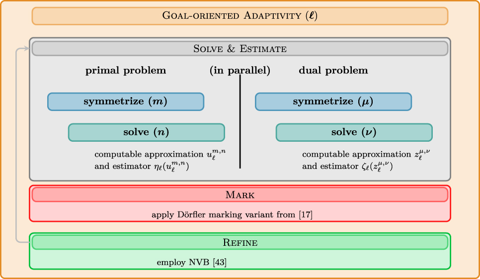
Schematic overview of the GOAISFEM algorithm with nested symmetrization and inexact solver.
Iteration counters and quasi-errors for the GOAISFEM algorithm. We note that for the combination of the index sets, the quasi-errors are extended to the full index set by the last available quasi-error. We refer to Section 3 for details on the iteration counters and index sets and to the beginning of Section 5 for a detailed description of the quasi-errors and their extension to the full index set
| Iteration | Mesh refinement | Symmetrization | Algebraic solver | Index set | Quasi-error | |||
|---|---|---|---|---|---|---|---|---|
| Running | Final | Running | Final | Running | Final | |||
| Primal | ℓ |
|
m |
|
|
|
|
|
| Dual | ℓ |
|
μ |
|
ν |
|
|
|
| Combined | ℓ |
|
k |
|
|
|
|
|
The first challenge in the analysis of the GOAISFEM algorithm consists of the nonlinear product structure attained by the combined quasi-error product as displayed in Table 1. The resulting nonlinear remainder term significantly complicates the proof compared to treating only the primal problem as in [28] and requires the application of a novel proof strategy from [33] that only utilizes summability of the remainder, denoted as tail-summability throughout. The second challenge arises from the combination of the primal and dual marking leading to a merged marked set. Thereby, either only the primal or only the dual estimator is guaranteed to satisfy the estimator reduction property. Since the estimator belongs to the quasi-error, this also leads to a failure of contraction for one of the two involved quasi-errors. While [29] solves this issue in the symmetric case, the additional symmetrization loop results in a more involved situation at hand. Adapting the novel approach of the tail-summability criterion from [33] enables the proof of full linear convergence and optimal complexity for the nonlinear quasi-error product in this paper. The analysis employs the generalized quasi-orthogonality from [34] to remedy the lack of a Pythagorean identity for nonsymmetric problems.
Our main result asserts full linear convergence of the quasi-error product
Note that, unlike [28], where full linear convergence is guaranteed only for sufficiently large ℓ ⩾ ℓ 0, the current result is stronger in the sense that the result holds for ℓ 0 = 0 owing to a generalized quasi-orthogonality from [34]. An immediate consequence of full linear convergence and the geometric series in Corollary 1 states that the rates with respect to the degrees of freedom coincide with the rates with respect to the cumulative computational work (i.e., computational time), i.e., for all r > 0, there holds
along the sequence of meshes
This means the convergence of the algorithm attains the optimal rate s + t with respect to the overall computational work, where
The remaining parts of the paper are organized as follows. The preliminary Section 2 introduces the model problem, the assumptions on the solvers, and the axioms of adaptivity from [9], including the general quasi-orthogonality from [34]. Following the algorithm in Section 3 and its contraction properties in Sections 4 and 5 presents full linear convergence as the first main result of this paper. This allows to prove optimal complexity in Section 6 as the second main result, which is underlined by the numerical experiments in Section 7 including a thorough investigation of the adaptivity parameters. The paper concludes with a summary in Section 8.
2 Setting
In this section, we introduce the problem and explain the key components needed to design the adaptive algorithm in Section 3.
2.1 Continuous model problem
Let
with a pointwise symmetric and positive definite diffusion matrix
We suppose that the bilinear form b(⋅, ⋅) from (5) is continuous and elliptic with respect to the norm
Then, the Lax–Milgram lemma proves existence and uniqueness of the solution u
⋆ to (5). An elementary compactness argument shows that (6) implies ellipticity of the principal part a(⋅, ⋅) and thus a(⋅, ⋅) is a scalar product on
In the present paper, we suppose that the quantity of interest G is linear and reads for given data g ∈ L
2(Ω) and
In order to guarantee well-definedness of the error estimator in Section 2.6 below, we suppose
2.2 Finite element discretization and discrete goal
For a polynomial degree
Since
It is well-known that conforming FEMs are quasi-optimal, i.e., there hold Céa-type estimates with constant C Céa = L/α
For arbitrary approximations
The definition of the discrete goal quantity by
We emphasize that (12) holds for any u
H
, z
H
and, in particular, for those stemming from an iterative solution step. Moreover, if
2.3 Zarantonello iteration
The discrete formulations (10) lead to positive definite, but nonsymmetric linear systems of equations. To reduce the formulation to symmetric and positive definite (SPD) problems, we follow previous own work [28] for the primal problem and employ the Zarantonello iteration [36]. Typically, the latter is used in the up-to-date proof of the Lax–Milgram lemma and also defines a linearization scheme for the treatment of a certain class of nonlinear elliptic PDEs (see, e.g., [33], [37], [38], [39]). In its core, it is a fixed-point method, thus also applicable in the nonsymmetric setting at hand. For a damping parameter δ > 0 and given
The Riesz–Fischer theorem (and also the Lax–Milgram lemma) guarantees existence and uniqueness of
The optimal value δ
opt = α/L
2 yields the minimal contraction value
2.4 Algebraic solver
A canonical candidate for solving (10) directly is a generalized minimal residual method [41], [42] with optimal preconditioner for the symmetric part. While this guarantees uniform contraction of the algebraic residuals in a discrete vector norm, the link between the algebraic residuals and the functional setting is still open [28]. Instead, after a symmetrization with the Zarantonello iteration, it remains to solve the SPD systems (13). Since large SPD problems are still computationally expensive and the exact solution cannot be computed in linear computational complexity, we employ an iterative algebraic solver whose iteration is expressed by the operator
To simplify notation, we shall identify ψ with its Riesz representative
2.5 Mesh refinement
The mesh refinement employs newest-vertex bisection (NVB). We refer to [43] for NVB with admissible initial triangulation
2.6 A posteriori error estimation
For a triangle
For any subset
as well as
For details on residual-based error estimators, we refer to [47], [48]. Throughout the paper, the index of the estimators refer to the underlying mesh, e.g., η
h
and ζ
h
on the refinement
Lemma 1
(see [9], Section 6.1]). The error estimators η
H
, ζ
H
from (16) satisfy the following properties with constants C
stab, C
rel, C
drel, C
mon > 0 and 0 < q
red < 1 for any triangulation
(A1) stability:
(A2) reduction:
(A3) reliability:
(A3+) discrete reliability:
(QM) quasi-monotonicity:
The constant C
rel depends only on the uniform γ-shape regularity of all
Reliability (A3) and stability (A1) verify
In combination with the estimate (12), we finally conclude for
which provides the core estimate of the proposed adaptive algorithm in Section 3 below.
The ellipticity of b(⋅, ⋅) from (7) ensures inf-sup stability of the elliptic problem at hand. Recall from [34] that inf-sup stability implies the generalized quasi-orthogonality, which will be an important tool in the subsequent analysis.
Proposition 1
(validity of quasi-orthogonality [34], Eq. (8)]). For any sequence
(A4) quasi-orthogonality: There exist constants C
orth > 0 and 0 < δ < 1 such that the corresponding Galerkin solutions
The constants C
orth and δ depend only on the dimension d, the elliptic bilinear form b(⋅, ⋅), and the chosen norm ||| ⋅ |||, but are independent of the spaces
3 Adaptive algorithm
In this section, we introduce our goal-oriented adaptive iteratively symmetrized algorithm. It utilizes specific stopping indices denoted by an underline, e.g.,
Algorithm 1
(GOAISFEM).
Input: Initial mesh
Adaptive loop: For all ℓ = 0, 1, 2, …, repeat the following steps (I)–(IV):
SOLVE & ESTIMATE (PRIMAL). For all m = 1, 2, 3, …, repeat (a)–(c):
Set
For all n = 1, 2, 3, …, repeat the following steps (i)–(ii):
Compute
Terminate n-loop and define
(19)
Terminate m-loop and define
(20)
SOLVE & ESTIMATE (DUAL). For all μ = 1, 2, 3, …, repeat (a)–(c):
Set
For all ν = 1, 2, 3, …, repeat the following steps (i)–(ii):
Compute
Terminate ν-loop and define
(21)
Terminate μ-loop and define
(22)
MARK. Determine sets
satisfying the following Dörfler criterion [1] with quasi-minimal cardinality
(23)As in [17], define the set of marked elements
REFINE. Generate the new mesh
Output: Sequences of successively refined triangulations
Remark 1.
(i) Although the primal loop (I) and dual loop (II) in Algorithm 1 are displayed sequentially, they are independent of each other. Therefore, a practical implementation will realize these iterations simultaneously since the system matrix is the same (thanks to the symmetrization step).
(ii) In order to investigate the asymptotic behavior, it is reasonable to analyze Algorithm 1 in the present formulation with infinitely many steps. We note that a practical implementation will terminate with
For the analysis of Algorithm 1, we define the index set
Furthermore, we require the following final indices and notice that these are consistent with those defined in Algorithm 1:
In addition, we set
Finally, we introduce the total step counter |⋅, ⋅, ⋅| defined for all
This definition indeed provides a lexicographic ordering on
Since
Lemma 2
(finite termination of algebraic solver [28], Lemma 3.2]). Independently of the algorithmic parameters δ, θ, λ
sym, and λ
alg, the innermost n- and ν-loops of Algorithm 1 always terminate. In particular,
4 A posteriori error analysis
Algorithm 1 does not provide the exact algebraic solutions
Lemma 3
(contraction of inexact Zarantonello iteration [28], Lemma 5.1]). Choose any damping parameter 0 < δ < δ ⋆ = 2α/L 2 to ensure the contraction (14) of the Zarantonello iteration and
Then, for arbitrary λ
sym > 0 and any
Moreover, for
The subsequent lemma gathers a posteriori error estimates following directly from the corresponding contraction of the symmetrization, algebraic solver, and the inexact Zarantonello iteration. Further details of the elementary proof are omitted.
Lemma 4
(stability and a posteriori error control). For all
Analogously, for all
For all
The analogous estimates are also valid for the dual variable.
Finally, the following lemma shows that in the case of finitely many mesh-refinement steps, the Zarantonello iteration does not terminate and one of the two exact continuous solutions is already the discrete solution to (10).
Lemma 5
(case of finite mesh-refinement steps). Suppose that the inexact Zarantonello iteration satisfies contraction (28) and that η and ζ satisfy (A1)–(A3). If
Proof.
By Lemma 2, we have
or
If (33) holds, then the inexact Zarantonello iterates
This proves that
Due to the contraction of the inexact Zarantonello iteration (28), we have the following a posteriori error estimates for the final iterates.
Lemma 6
(stability of final iterates). Suppose that the inexact Zarantonello iteration satisfies (28). Then, for all
Proof.
For
Let
This and with the contraction of the exact Zarantonello iteration (14) result in
Consequently, the combination of (39) and (35) validates (36) via
The estimate (39) also implies (37), because
The same arguments prove the estimates for the dual variable and conclude the proof.□
The subsequent lemma states the estimator reduction for only one of the two error estimators. This poses a significant challenge in the proof of full linear convergence due to the required contraction of the nonlinear quasi-error product in Lemma 8 below.
Lemma 7
(estimator reduction and stability). Define the constant
If the dual error estimator satisfies the Dörfler criterion, i.e.,
Proof.
For
The Dörfler marking in Algorithm 1(III) for the primal error estimator η and
For
For
The proof holds verbatim in the case of Dörfler marking for the dual error estimator, albeit with reversed roles. This concludes the proof.□
5 Full linear convergence
This section presents full linear convergence of Algorithm 1 as the first main result of this work. Recall the goal-error estimate from (17) motivating the product structure of the respective primal and dual error components. Thus, we define the quasi-errors
The quasi-errors naturally extend to the full index set
The following theorem asserts full linear convergence of the quasi-error product.
Theorem 1
(full linear convergence). Suppose that the estimators η and ζ satisfy (A1)–(A3) and (QM) and suppose (A4). Recall
Then, for arbitrary marking parameter 0 < θ ⩽ 1 and any solver parameters λ
sym > 0 and
The constants C
lin and q
lin depend only on C
stab, C
rel, C
mon, C
orth, C
Céa, θ, q
red, q
sym,
Three lemmas are required to prove Theorem 1. The characterization of R-linear convergence from [33], Lemma 5 and 10] is the primary tool for the proof of Theorem 1; see (70) below. The proof of Theorem 1 departs with the contraction of the quasi-error for the final iterates of the inexact Zarantonello loop up to a remainder on the mesh level ℓ. To this end, we define the simplified weighted quasi-error
where γ > 0 is a free parameter chosen in (51) below. This quasi-error quantity satisfies contraction up to a tail-summable remainder due to estimator reduction (40), (41).
Lemma 8
(contraction in mesh level up to tail-summable remainder). Under the assumptions of Theorem 1, there exists 0 < q < 1 such that the quasi-error product H ℓ Z ℓ from (48) satisfies contraction up to a remainder R ℓ ⩾ 0,
The remainder R ℓ satisfies
Proof.
The proof consists of four steps.
Step 1 (choice of constants). Recall the constants 0 < q(θ) < 1 from Lemma 7 and λ
⋆ > 0 and
Elementary calculations show that the choice of
ensures
Consequently, we have q(θ) C(γ,λ)2 < 1 and thus
Step 2 (contraction of
H
ℓ
and
Z
ℓ
). Abbreviate λ: = λ
alg λ
sym. Recall that marking in Algorithm 1(III) ensures that the estimate (40) or (41) hold. If (40) is satisfied, the quasi-contraction of the inexact Zarantonello iteration (29) for the final iterate, the stability estimate (35), and the estimator reduction (40) lead, for all
The same arguments yield, for all
For
If (41) is satisfied, we obtain the same estimate with reversed roles in the derivation.
Step 3 (quasi-monotonicity of H
ℓ
and Z
ℓ
). The Céa estimate (11), nestedness of the discrete spaces, reliability (A3), quasi-monotonicity (QM), stability (A1), and the definition (48) prove, for all
where the hidden constants depend only on γ −1, C Céa, C stab, C rel, and C mon.
Similarly to (53), the inexact Zarantonello contraction (29), stability (A1), and the stability estimate (36) yield for
The choice of λ ⩽ λ ⋆ with λ ⋆ from (46) ensures
With
Hence, we have quasi-monotonicity of the quasi-error
The same argument proves
Step 4 (contraction of H ℓ Z ℓ up to tail-summable remainder). Define
The contraction (55) proves the quasi-contraction (49) via
The remainder term R ℓ can be estimated via (56) and the Young inequality by
Thus, the quasi-monotonicity (60) verifies
Quasi-orthogonality (A4), reliability (A3), and the estimates (56) imply, for all
Using (61), the quasi-monotonicity (60), and (62), we conclude the proof of (50), for all
□
The tail-summability in ℓ provides the basis for the proof of tail-summability on the mesh level ℓ together with the Zarantonello symmetrization index k for the final iterates of the algebraic solver. The main ingredients in the proof of tail-summability in (ℓ, k) are Lemma 8 and the following quasi-contraction in the symmetrization index k.
Lemma 9
(quasi-contraction of inexact Zarantonello symmetrization). There holds
Proof.
First, we note that the a posteriori error control (31) and the stopping criteria of the algebraic solver (19) and of the symmetrization (20) lead, for
Since the two notions of quasi-errors H
ℓ
and
For
Moreover, for
For
Since
Furthermore, there holds
where the hidden constant depends only on C stab, λ sym, and q sym.
Nested iteration
A multiplication of the two previous estimates proves (64).□
Finally, the quasi-contraction in (ℓ, k) from Lemma 9 together with a quasi-contraction in the algebraic solver index j leads to tail-summability in (ℓ, k, j).
Lemma 10
(quasi-contraction and stability by algebraic solver). There holds
and, with the abbreviation (m − 1)+: = max{m − 1, 0},
Proof.
We recall that
Therewith, we derive (68).
The combination of a posteriori error control (30) for the exact Zarantonello iteration, for the algebraic solver (31), and the failure of the stopping criterion (19) in Algorithm 1(I.b.ii) for the algebraic solver proves, for
For
For
Furthermore, we have
where the hidden constant depends only on
Ultimately, synthesizing the preceding lemmas yields tail-summability of the quasi-error product and thus leads to the following proof of Theorem 1.
Proof of Theorem 1.
The proof consists of four steps.
Step 1 (tail-summability in mesh level
ℓ
). We apply the tail-summability criterion from [33], Lemma 5] to the sequences a
ℓ
:= H
ℓ
Z
ℓ
and
Indeed, contraction up to a remainder from (49), the estimate of the remainder from (50), and the quasi-monotonicity of H ℓ and Z ℓ from (60) validate the assumptions of the tail-summability criterion (70) and lead to tail-summability
Step 2 (tail-summability in (ℓ, k)). For
Step 3 (tail-summability in (ℓ, k, j)
). Finally, for all
Step 4. Since the index set
6 Optimal complexity of Algorithm 1
Full linear convergence (47) has a simple but crucial consequence. Using a geometric series argument, one can prove that the cumulative computational cost up to a given level is bounded by the cost of the said level; see [33], Corollary 14], where only the primal quasi-error
Corollary 1
(rates = complexity [33], Corollary 14]). Suppose the assumptions of Theorem 1. For all r > 0, the output
with the constant
While Theorem 1 only concerns R-linear convergence, a sufficiently small choice of the adaptivity parameters θ, λ sym, and λ alg even guarantees the optimal convergence rate r = s + t with respect to computational cost, i.e., the overall computational time. Here, we suppose that the primal solution u ⋆ to (5) can be approximated at rate s and the dual solution z ⋆ to (8) can be approximated at rate t. To formalize this idea, we introduce the notion of approximation classes [3], [4], [5], [9]. For s, t > 0, define
where η
opt(⋅) and ζ
opt(⋅) denote the estimator values for the exact discrete solutions
Theorem 2
(optimal complexity). Suppose that the estimators η and ζ satisfy (A1)–(A3+) and (QM) and suppose quasi-orthogonality (A4). Recall
Suppose that θ, λ sym, and λ alg are sufficiently small in the sense of
Then, Algorithm 1 guarantees, for all s, t > 0, that
The constant C
opt depends only on C
stab, C
rel, C
drel, C
mark, C
mesh, C
lin, q
lin,
The proof of Theorem 2 employs the following result from [50] providing estimator equivalence between the (unavailable) estimators for the exact discrete solutions
Lemma 11
(estimator equivalence [50], Lemma 15]). Recall the constants
Proof of Theorem 2.
By Corollary 1, it suffices to prove that, for any s, t > 0,
Since the inequality becomes trivial if either
Step 1. With
For
and consequently with (79a) to
Note that the stopping criteria (20) and (22) lead to
and with (64) to
Hence, the combination of (80) and (81) reads
Step 2. Recall from [29], Theorem 8] that the set
with the constant C mark ⩾ 1 from Algorithm 1.
Step 3. Let
NVB refinement satisfies the mesh-closure estimate [9], Eq. (2.9)] reading,
where C
mesh > 1 depends only on
Rearranging the terms and noting that
Moreover, full linear convergence (47) proves that
We recall from [35], Lemma 22] that, for all
This shows, for all
and concludes the proof of (78).□
7 Numerical examples
In this section, we present numerical experiments using the open source software package MooAFEM [51].[1] In the following, Steps (I) and (II) of Algorithm 1 employ the optimal hp-robust local multigrid method from [32] as an algebraic solver. If not explicitly stated otherwise, we choose the parameters θ = 0.5, δ = 0.5, λ sym = λ alg = 0.7 in Algorithm 1 throughout the numerical experiments.
7.1 Singularity in the goal functional
The first model problem is a nonsymmetric variant of the benchmark problem from [29], Section 4.1] with a singularity only in the goal functional. On the unit square
where the right-hand side is chosen such that the exact solution u ⋆ reads
Consider g = 0 and g = χ K (1,0) ⊤ in the quantity of interest
Figure 2 (left) displays a mesh generated by Algorithm 1 and the support K of g . The error estimator captures and resolves the two point singularities induced by G.
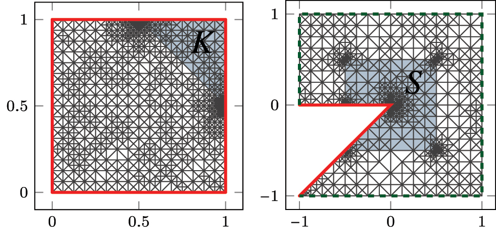
Left: Mesh
7.2 Geometric singularity and strong convection
The second benchmark problem investigates
Consider g = 0 and g = χ S (1,1) ⊤ in the quantity of interest
The exact solution u
⋆ is not known analytically in this case so that we do not have access to the exact goal error
7.2.1 Optimality of Algorithm 1
Figure 3 displays the estimator product
of Algorithm 1 for polynomial degree p = 2 with
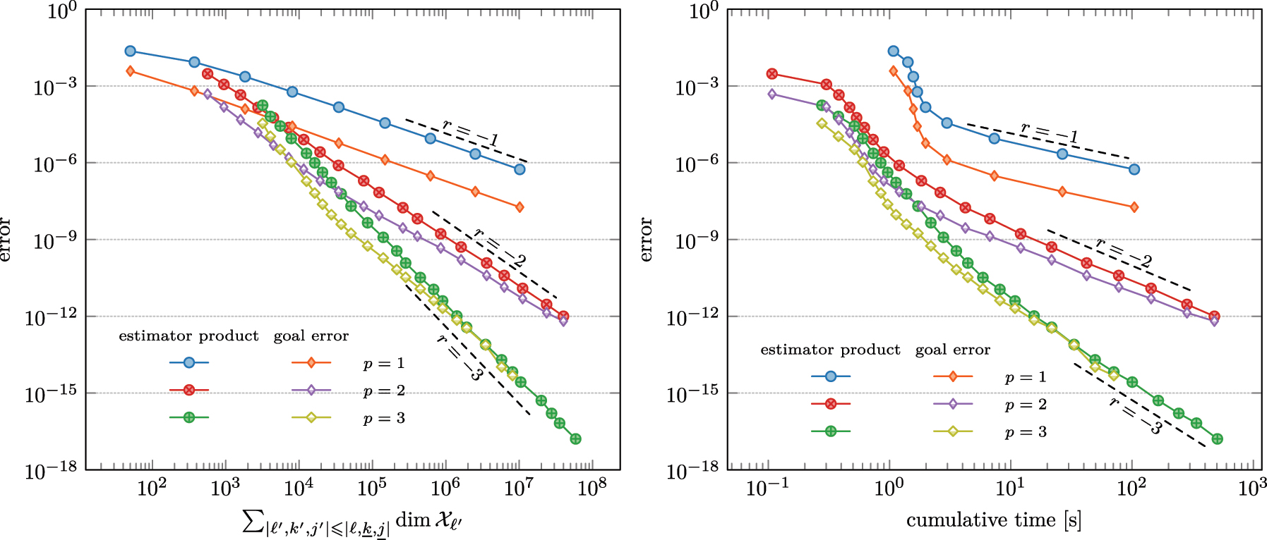
Convergence history plot of estimator product
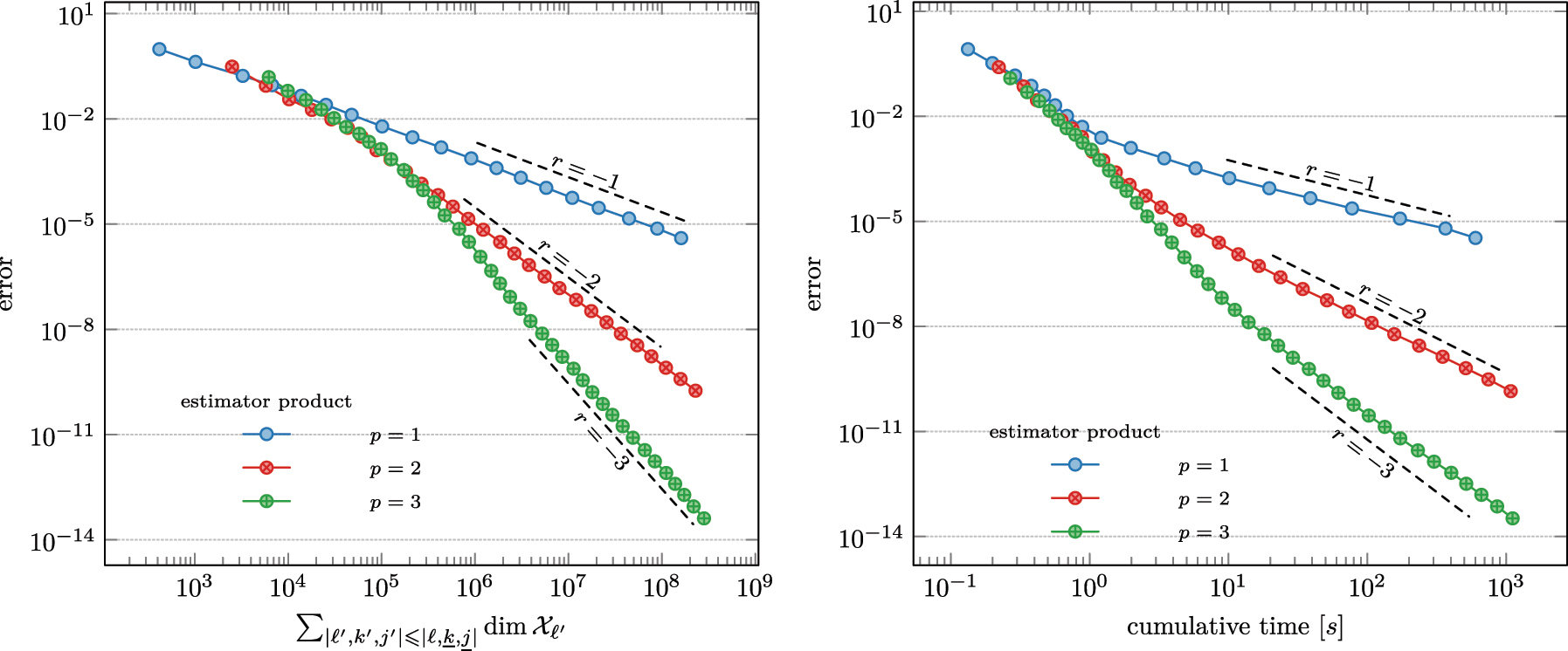
Convergence history plot of estimator product
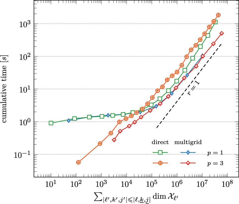
Comparison of cumulative time of the local multigrid solver with the Matlab built-in direct solver mldivide with respect to the cumulative computational cost for the benchmark problem (89).
Optimal selection of parameters with respect to the cumulative computational costs (overall computation time in seconds) for the experiment (88) with fixed polynomial degree p = 2 and δ = 0.5. For comparison, the table displays the value of the weighted costs from (90) (in 10−7) with overall stopping criterion
| ×10−7 | θ = 0.1 | θ = 0.3 | θ = 0.5 | ||||||||||||
|---|---|---|---|---|---|---|---|---|---|---|---|---|---|---|---|
| λ alg/λ sym | 0.1 | 0.3 | 0.5 | 0.7 | 0.9 | 0.1 | 0.3 | 0.5 | 0.7 | 0.9 | 0.1 | 0.3 | 0.5 | 0.7 | 0.9 |
| 0.1 | 38.7 | 33.4 | 29.6 | 22.1 | 24.4 | 10.2 | 5.12 | 4.90 | 4.83 | 4.74 | 6.18 | 4.48 | 4.66 | 4.89 | 5.25 |
| 0.3 | 36.2 | 24.7 | 24.5 | 21.8 | 23.1 | 7.28 | 4.98 | 3.53 | 3.27 | 3.26 | 4.18 | 4.54 | 4.79 | 5.01 | 5.13 |
| 0.5 | 24.3 | 24.7 | 24.7 | 23.4 | 23.6 | 5.84 | 3.64 | 3.39 | 3.27 | 3.37 | 3.41 | 2.71 | 2.52 | 2.49 | 2.68 |
| 0.7 | 24.1 | 24.8 | 23.8 | 22.2 | 24.0 | 4.95 | 3.59 | 3.30 | 3.25 | 3.42 | 2.74 | 2.35 | 2.41 | 2.24 | 2.46 |
| 0.9 | 23.5 | 24.6 | 22.3 | 24.4 | 23.8 | 4.90 | 3.58 | 3.29 | 3.26 | 3.41 | 2.81 | 2.30 | 2.43 | 2.27 | 2.41 |
| θ = 0.7 | θ = 0.8 | θ = 0.9 | |||||||||||||
| 0.1 | 5.82 | 5.18 | 5.43 | 5.40 | 5.93 | 8.53 | 6.10 | 7.31 | 6.67 | 7.77 | 11.6 | 8.86 | 9.12 | 9.87 | 9.97 |
| 0.3 | 4.65 | 4.86 | 5.35 | 5.98 | 6.67 | 6.27 | 5.92 | 7.20 | 7.46 | 7.57 | 8.62 | 8.40 | 9.27 | 10.6 | 11.5 |
| 0.5 | 3.69 | 2.89 | 2.88 | 2.95 | 3.13 | 5.09 | 3.61 | 3.66 | 3.63 | 3.66 | 7.27 | 5.32 | 4.84 | 4.93 | 5.12 |
| 0.7 | 2.99 | 2.56 | 2.64 | 2.62 | 2.89 | 3.75 | 3.12 | 3.23 | 3.03 | 3.11 | 4.58 | 3.95 | 4.04 | 4.43 | 4.79 |
| 0.9 | 2.89 | 2.49 | 2.65 | 2.66 | 2.89 | 3.79 | 3.11 | 3.19 | 3.13 | 3.27 | 4.67 | 4.06 | 4.16 | 4.35 | 4.61 |
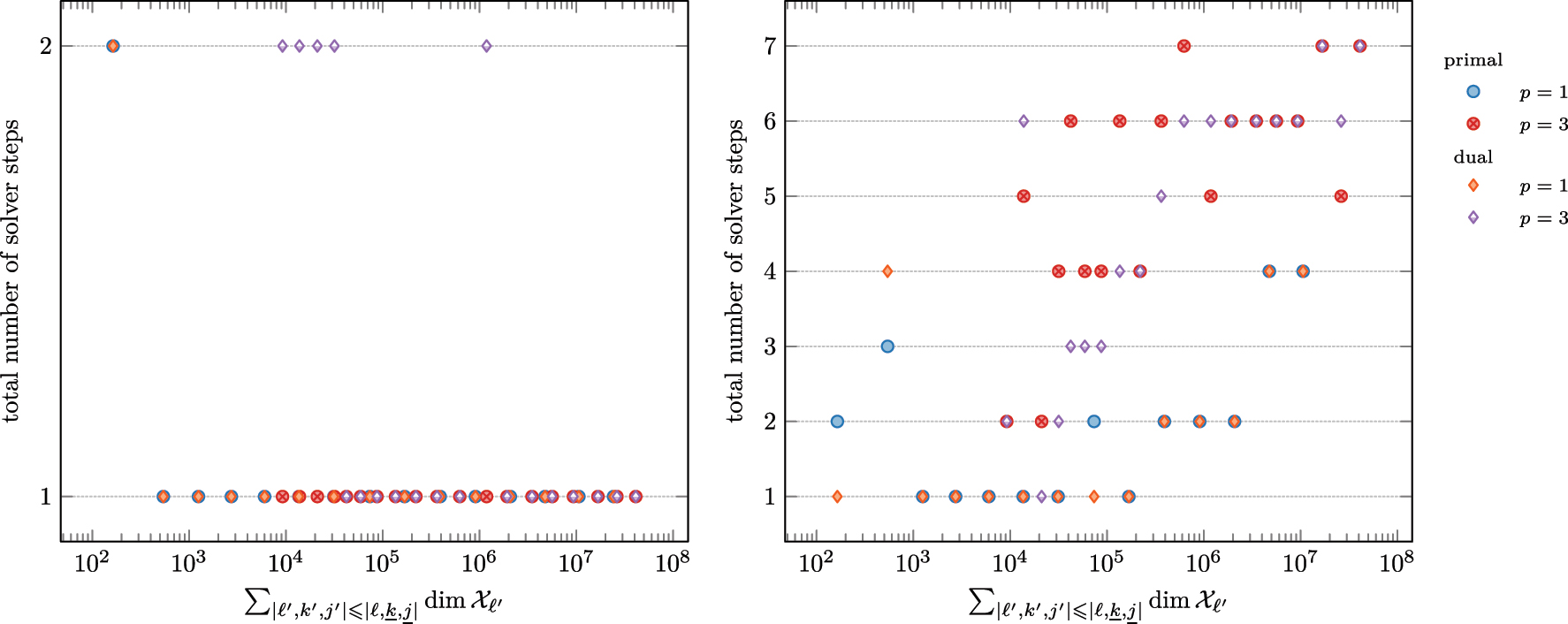
Finally, in Figure 6, we display the number of total solver steps
8 Summary
In this work, we developed a cost-optimal goal-oriented adaptive finite element method for the efficient computation of the quantity of interest G(u
⋆) with solution u
⋆ to the general second-order linear elliptic partial differential equation (4). Since the current analysis of iterative algebraic solvers for nonsymmetric systems with optimal preconditioner only leads to contraction of the residual in a vector norm, we proposed a nested iterative solver for the primal and dual problem in parallel. The strategy consists of the Zarantonello iteration (13) as an outer solver loop and an optimal multigrid solver for the arising SPD system as an innermost solver loop. In recent own work [33], we have shown that the link between convergence rates with respect to the degrees of freedom and the total computational cost is full linear convergence of the quasi-error
-
Research ethics: Not applicable.
-
Author contributions: All authors have accepted responsibility for the entire content of this manuscript and approved its submission.
-
Use of Large Language Models, AI and Machine Learning Tools: None declared.
-
Competing interests: The authors state no conflict of interest.
-
Research funding: This research was funded in whole or in part by the Austrian Science Fund (FWF) through [10.55776/F65], [10.55776/I6802], and [10.55776/P33216]. For open access purposes, the author has applied a CC BY public copyright license to any author accepted manuscript version arising from this submission. Additionally, Maximilian Brunner and Julian Streitberger are supported by the Vienna School of Mathematics.
-
Data availability: Not applicable.
References
[1] W. Dörfler, “A convergent adaptive algorithm for Poisson’s equation,” SIAM J. Numer. Anal., vol. 33, no. 3, pp. 1106–1124, 1996. https://doi.org/10.1137/0733054.Search in Google Scholar
[2] P. Morin, R. H. Nochetto, and K. G. Siebert, “Data oscillation and convergence of adaptive FEM,” SIAM J. Numer. Anal., vol. 38, no. 2, pp. 466–488, 2000. https://doi.org/10.1137/s0036142999360044.Search in Google Scholar
[3] P. Binev, W. Dahmen, and R. DeVore, “Adaptive finite element methods with convergence rates,” Numer. Math., vol. 97, no. 2, pp. 219–268, 2004. https://doi.org/10.1007/s00211-003-0492-7.Search in Google Scholar
[4] R. Stevenson, “Optimality of a standard adaptive finite element method,” Found. Comput. Math., vol. 7, no. 2, pp. 245–269, 2007. https://doi.org/10.1007/s10208-005-0183-0.Search in Google Scholar
[5] J. M. Cascón, C. Kreuzer, R. H. Nochetto, and K. G. Siebert, “Quasi-optimal convergence rate for an adaptive finite element method,” SIAM J. Numer. Anal., vol. 46, no. 5, pp. 2524–2550, 2008. https://doi.org/10.1137/07069047x.Search in Google Scholar
[6] C. Kreuzer and K. G. Siebert, “Decay rates of adaptive finite elements with Dörfler marking,” Numer. Math., vol. 117, no. 4, pp. 679–716, 2011. https://doi.org/10.1007/s00211-010-0324-5.Search in Google Scholar
[7] J. M. Cascón and R. H. Nochetto, “Quasioptimal cardinality of AFEM driven by nonresidual estimators,” IMA J. Numer. Anal., vol. 32, no. 1, pp. 1–29, 2012. https://doi.org/10.1093/imanum/drr014.Search in Google Scholar
[8] M. Feischl, T. Führer, and D. Praetorius, “Adaptive FEM with optimal convergence rates for a certain class of nonsymmetric and possibly nonlinear problems,” SIAM J. Numer. Anal., vol. 52, no. 2, pp. 601–625, 2014. https://doi.org/10.1137/120897225.Search in Google Scholar
[9] C. Carstensen, M. Feischl, M. Page, and D. Praetorius, “Axioms of adaptivity,” Comput. Math. Appl., vol. 67, no. 6, pp. 1195–1253, 2014. https://doi.org/10.1016/j.camwa.2013.12.003.Search in Google Scholar PubMed PubMed Central
[10] R. Becker and R. Rannacher, “An optimal control approach to a posteriori error estimation in finite element methods,” Acta Numer., vol. 10, pp. 1–102, 2001. https://doi.org/10.1017/s0962492901000010.Search in Google Scholar
[11] W. Bangerth and R. Rannacher, Adaptive Finite Element Methods for Differential Equations, Basel, Springer Science & Business Media, 2003.10.1007/978-3-0348-7605-6Search in Google Scholar
[12] K. Eriksson, D. Estep, P. Hansbo, and C. Johnson, “Introduction to adaptive methods for differential equations,” Acta Numer., vol. 4, pp. 105–158, 1995. https://doi.org/10.1017/s0962492900002531.Search in Google Scholar
[13] M. B. Giles and E. Süli, “Adjoint methods for PDEs: a posteriori error analysis and postprocessing by duality,” Acta Numer., vol. 11, pp. 145–236, 2002. https://doi.org/10.1017/cbo9780511550140.003.Search in Google Scholar
[14] M. S. Mommer and R. Stevenson, “A goal-oriented adaptive finite element method with convergence rates,” SIAM J. Numer. Anal., vol. 47, no. 2, pp. 861–886, 2009. https://doi.org/10.1137/060675666.Search in Google Scholar
[15] R. Becker, E. Estecahandy, and D. Trujillo, “Weighted marking for goal-oriented adaptive finite element methods,” SIAM J. Numer. Anal., vol. 49, no. 6, pp. 2451–2469, 2011. https://doi.org/10.1137/100794298.Search in Google Scholar
[16] M. Feischl, G. Gantner, A. Haberl, D. Praetorius, and T. Führer, “Adaptive boundary element methods for optimal convergence of point errors,” Numer. Math., vol. 132, no. 3, pp. 541–567, 2016. https://doi.org/10.1007/s00211-015-0727-4.Search in Google Scholar
[17] M. Feischl, D. Praetorius, and K. G. van der Zee, “An abstract analysis of optimal goal-oriented adaptivity,” SIAM J. Numer. Anal., vol. 54, no. 3, pp. 1423–1448, 2016. https://doi.org/10.1137/15m1021982.Search in Google Scholar
[18] M. Holst and S. Pollock, “Convergence of goal-oriented adaptive finite element methods for nonsymmetric problems,” Numer. Methods Partial Differ. Equ., vol. 32, no. 2, pp. 479–509, 2016. https://doi.org/10.1002/num.22002.Search in Google Scholar
[19] R. Becker, M. Innerberger, and D. Praetorius, “Optimal convergence rates for goal-oriented FEM with quadratic goal functional,” Comput. Methods Appl. Math., vol. 21, no. 2, pp. 267–288, 2021. https://doi.org/10.1515/cmam-2020-0044.Search in Google Scholar
[20] R. Becker, M. Brunner, M. Innerberger, J. M. Melenk, and D. Praetorius, “Rate-optimal goal-oriented adaptive FEM for semilinear elliptic PDEs,” Comput. Math. Appl., vol. 118, pp. 18–35, 2022. https://doi.org/10.1016/j.camwa.2022.05.008.Search in Google Scholar
[21] B. Endtmayer, U. Langer, and T. Wick, “Multigoal-oriented error estimates for non-linear problems,” J. Numer. Math., vol. 27, no. 4, pp. 215–236, 2019. https://doi.org/10.1515/jnma-2018-0038.Search in Google Scholar
[22] B. Endtmayer, U. Langer, and T. Wick, “Two-side a posteriori error estimates for the dual-weighted residual method,” SIAM J. Sci. Comput., vol. 42, no. 1, pp. A371–A394, 2020. https://doi.org/10.1137/18m1227275.Search in Google Scholar
[23] V. Dolejší, O. Bartoš, and F. Roskovec, “Goal-oriented mesh adaptation method for nonlinear problems including algebraic errors,” Comput. Math. Appl., vol. 93, pp. 178–198, 2021. https://doi.org/10.1016/j.camwa.2021.04.004.Search in Google Scholar
[24] A. Cohen, W. Dahmen, and R. DeVore, “Adaptive wavelet methods for elliptic operator equations: convergence rates,” Math. Comput., vol. 70, no. 233, pp. 27–75, 2001. https://doi.org/10.1090/s0025-5718-00-01252-7.Search in Google Scholar
[25] A. Cohen, W. Dahmen, and R. DeVore, “Adaptive wavelet schemes for nonlinear variational problems,” SIAM J. Numer. Anal., vol. 41, no. 5, pp. 1785–1823, 2003. https://doi.org/10.1137/s0036142902412269.Search in Google Scholar
[26] C. Carstensen and J. Gedicke, “An adaptive finite element eigenvalue solver of asymptotic quasi-optimal computational complexity,” SIAM J. Numer. Anal., vol. 50, no. 3, pp. 1029–1057, 2012. https://doi.org/10.1137/090769430.Search in Google Scholar
[27] G. Gantner, A. Haberl, D. Praetorius, and S. Schimanko, “Rate optimality of adaptive finite element methods with respect to overall computational costs,” Math. Comput., vol. 90, no. 331, pp. 2011–2040, 2021. https://doi.org/10.1090/mcom/3654.Search in Google Scholar
[28] M. Brunner, M. Innerberger, A. Miraçi, D. Praetorius, J. Streitberger, and P. Heid, “Adaptive FEM with quasi-optimal overall cost for nonsymmetric linear elliptic PDEs,” IMA J. Numer. Anal., vol. 44, no. 3, pp. 1560–1596, 2024. https://doi.org/10.1093/imanum/drad039.Search in Google Scholar
[29] R. Becker, G. Gantner, M. Innerberger, and D. Praetorius, “Goal-oriented adaptive finite element methods with optimal computational complexity,” Numer. Math., vol. 153, no. 1, pp. 111–140, 2023. https://doi.org/10.1007/s00211-022-01334-8.Search in Google Scholar PubMed PubMed Central
[30] J. Wu and H. Zheng, “Uniform convergence of multigrid methods for adaptive meshes,” Appl. Numer. Math., vol. 113, pp. 109–123, 2017. https://doi.org/10.1016/j.apnum.2016.11.005.Search in Google Scholar
[31] L. Chen, R. H. Nochetto, and J. Xu, “Optimal multilevel methods for graded bisection grids,” Numer. Math., vol. 120, no. 1, pp. 1–34, 2012. https://doi.org/10.1007/s00211-011-0401-4.Search in Google Scholar
[32] M. Innerberger, A. Miraçi, D. Praetorius, and J. Streitberger, “hp-robust multigrid solver on locally refined meshes for FEM discretizations of symmetric elliptic PDEs,” ESAIM: Math. Modell. Numer. Anal., vol. 58, no. 1, pp. 247–272, 2024. https://doi.org/10.1051/m2an/2023104.Search in Google Scholar
[33] P. Bringmann, M. Feischl, A. Miraçi, D. Praetorius, and J. Streitberger, “On full linear convergence and optimal complexity of adaptive FEM with inexact solver,”arXiv:2311.15738, 2023. https://doi.org/10.48550/arXiv.2311.15738.Search in Google Scholar
[34] M. Feischl, “Inf-sup stability implies quasi-orthogonality,” Math. Comput., vol. 91, no. 337, pp. 2059–2094, 2022. https://doi.org/10.1090/mcom/3748.Search in Google Scholar
[35] A. Bespalov, A. Haberl, and D. Praetorius, “Adaptive FEM with coarse initial mesh guarantees optimal convergence rates for compactly perturbed elliptic problems,” Comput. Methods Appl. Mech. Eng., vol. 317, pp. 318–340, 2017. https://doi.org/10.1016/j.cma.2016.12.014.Search in Google Scholar
[36] E. Zarantonello, “Solving functional equations by contractive averaging, math,” Res. Cent. Rep., vol. 160, 1960.Search in Google Scholar
[37] S. Congreve and T. P. Wihler, “Iterative Galerkin discretizations for strongly monotone problems,” J. Comput. Appl. Math., vol. 311, pp. 457–472, 2017. https://doi.org/10.1016/j.cam.2016.08.014.Search in Google Scholar
[38] G. Gantner, A. Haberl, D. Praetorius, and B. Stiftner, “Rate optimal adaptive FEM with inexact solver for nonlinear operators,” IMA J. Numer. Anal., vol. 38, no. 4, pp. 1797–1831, 2018. https://doi.org/10.1093/imanum/drx050.Search in Google Scholar
[39] A. Haberl, D. Praetorius, S. Schimanko, and M. Vohralík, “Convergence and quasi-optimal cost of adaptive algorithms for nonlinear operators including iterative linearization and algebraic solver,” Numer. Math., vol. 147, no. 3, pp. 679–725, 2021. https://doi.org/10.1007/s00211-021-01176-w.Search in Google Scholar
[40] E. Zeidler, Nonlinear Functional Analysis and its Applications. Part II/A, New York, Springer-Verlag, 1990.10.1007/978-1-4612-0981-2Search in Google Scholar
[41] Y. Saad, Iterative Methods for Sparse Linear Systems, 2nd ed. Philadelphia, PA, Society for Industrial and Applied Mathematics, 2003.10.1137/1.9780898718003Search in Google Scholar
[42] Y. Saad and M. H. Schultz, “GMRES: a generalized minimal residual algorithm for solving nonsymmetric linear systems,” SIAM J. Sci. Comput., vol. 7, no. 3, pp. 856–869, 1986. https://doi.org/10.1137/0907058.Search in Google Scholar
[43] R. Stevenson, “The completion of locally refined simplicial partitions created by bisection,” Math. Comput., vol. 77, no. 261, pp. 227–241, 2008. https://doi.org/10.1090/s0025-5718-07-01959-x.Search in Google Scholar
[44] M. Aurada, M. Feischl, T. Führer, M. Karkulik, and D. Praetorius, “Energy norm based error estimators for adaptive BEM for hypersingular integral equations,” Appl. Numer. Math., vol. 95, pp. 15–35, 2015. https://doi.org/10.1016/j.apnum.2013.12.004.Search in Google Scholar
[45] M. Karkulik, D. Pavlicek, and D. Praetorius, “On 2D newest vertex bisection: optimality of mesh-closure and H1-stability of L2-projection,” Constr. Approx., vol. 38, no. 2, pp. 213–234, 2013. https://doi.org/10.1007/s00365-013-9192-4.Search in Google Scholar
[46] L. Diening, L. Gehring, and J. Storn, “Adaptive Mesh Refinement for Arbitrary Initial Triangulations,”arXiv.2306.02674, 2023.Search in Google Scholar
[47] M. Ainsworth and J. T. Oden, A Posteriori Error Estimation in Finite Element Analysis, Ser. Pure and Applied Mathematics, New York, Wiley-Interscience, 2000.10.1002/9781118032824Search in Google Scholar
[48] R. Verfürth, “A posteriori error estimation and adaptive mesh-refinement techniques,” in Proceedings of the Fifth International Congress on Computational and Applied Mathematics (Leuven, 1992), vol. 50, pp. 67–83, 1994.10.1016/0377-0427(94)90290-9Search in Google Scholar
[49] C.-M. Pfeiler and D. Praetorius, “Dörfler marking with minimal cardinality is a linear complexity problem,” Math. Comput., vol. 89, no. 326, pp. 2735–2752, 2020. https://doi.org/10.1090/mcom/3553.Search in Google Scholar
[50] M. Brunner, M. Innerberger, A. Miraçi, D. Praetorius, J. Streitberger, and P. Heid, “Corrigendum to: adaptive FEM with quasi-optimal overall cost for nonsymmetric linear elliptic PDEs,” IMA J. Numer. Anal., vol. 44, no. 3, pp. 1903–1909, 2024. https://doi.org/10.1093/imanum/drad103.Search in Google Scholar
[51] M. Innerberger and D. Praetorius, “MooAFEM: an object oriented matlab code for higher-order adaptive FEM for (nonlinear) elliptic PDEs,” Appl. Math. Comput., vol. 442, Art. no. 127731, 2023.10.1016/j.amc.2022.127731Search in Google Scholar
© 2024 the author(s), published by De Gruyter, Berlin/Boston
This work is licensed under the Creative Commons Attribution 4.0 International License.
Articles in the same Issue
- Frontmatter
- Effective highly accurate time integrators for linear Klein–Gordon equations across the scales
- Optimal complexity of goal-oriented adaptive FEM for nonsymmetric linear elliptic PDEs
- Stability and error analysis of a semi-implicit scheme for incompressible flows with variable density and viscosity
- Error analysis of virtual element method for the Poisson–Boltzmann equation