
From asymptotic distribution and vague convergence to uniform convergence, with numerical applications
-
Giovanni Barbarino
 und
Paris Vassalos
und
Paris Vassalos

Abstract
Let
1 Introduction
Throughout this paper, a matrix-sequence is a sequence of the form
where the entries …, f −2, f −1, f 0, f 1, f 2, … are k × k matrices (blocks) for some k ⩾ 1. If k = 1, then (1.1) is a classical (scalar) Toeplitz matrix. The nth section of (1.1) is the matrix defined by
A case of special interest arises when the entries f
k
are the Fourier coefficients of a function
where the integrals are computed componentwise. In this case, the matrix A
n
in (1.2) is denoted by T
n
(f) and is referred to as the nth (block) Toeplitz matrix generated by f. The asymptotic singular value and eigenvalue distributions of the Toeplitz sequence
An important concept related to matrix-sequences is the notion of asymptotic spectral (or eigenvalue) distribution. After the publication of Tyrtyshnikov’s paper in 1996 [11], there has been an ever growing interest in this topic, which led, among others, to the birth of GLT sequences [17], [18], [19]. The reasons behind this widespread interest are not purely academic, because the asymptotic spectral distribution has significant practical implications. For example, suppose that
Before proceeding further, let us introduce the formal definition of asymptotic singular value and eigenvalue distribution. Let
Definition 1.1
(asymptotic singular value and eigenvalue distribution of a matrix-sequence). Let
We say that
(1.3)In this case, f is called the eigenvalue (or spectral) symbol of
We say that
(1.4)In this case, f is called the singular value symbol of
We remark that Definition 1.1 is well-posed as the functions
Definition 1.2
(asymptotic distribution of a sequence of finite multisets of numbers). Let
In the previous literature, it has often been claimed that the informal meaning behind the asymptotic spectral distribution (1.3) is the following [5], Rem. 2.9]: assuming that there exist k a.e. continuous functions
for n large enough; similarly, if d = 2, d n = n 2 k, and Ω = [a 1, b 1] × [a 2, b 2], then, assuming we have no outliers, the eigenvalues of A n are approximately equal to
for n large enough; and so on for d ⩾ 3. In the case where d = k = 1, Ω = [a, b] is a bounded interval,
where ‖ ⋅ ‖∞ is the usual ∞-norm of vectors,
λ
(A
n
) is the properly sorted vector of eigenvalues of A
n
, f(
x
n
) is the vector of samples
In this paper, using the concept of monotone rearrangement (quantile function) and matrix analysis arguments from the theory of GLT sequences, we provide deeper insights into the notion of asymptotic spectral distribution by presenting precise mathematical formulations and proofs of the informal meaning behind (1.3) that are more general than [26], Th. 1.3]. Our formulations are made in terms of uniform convergence to 0 of differences of vectors, in complete analogy with (1.5).
In our first main result (Theorem 2.1), we extend [26], Th. 1.3] by formulating and proving the informal meaning behind (1.3) in the case where d ⩾ 1 and the domain Ω of the spectral symbol f is a Peano–Jordan measurable set (i.e., a bounded set with μ d (∂Ω) = 0). In Corollary 2.1, we prove (a slightly more general version of) [26], Th. 1.3] as a corollary of Theorem 2.1.
In our second main result (Theorem 2.2), we prove for d = 1 that Theorem 2.1 can be strengthened in the case where the spectrum of A n is contained in the image of f for every n and f satisfies some mild assumptions. More precisely, in this case we prove that the eigenvalues of A n are exact samples of f over an asymptotically uniform grid (see Section 2 for the corresponding definition).
In our last main result (Theorem 2.3), we extend [26], Th. 1.3] by formulating and proving the informal meaning behind (1.3) in the case where k ⩾ 1, i.e., the spectral symbol f is a matrix-valued function.
The results herein, including the main Theorems 2.1–2.3, are actually formulated in terms of asymptotic distributions of sequences of finite multisets of numbers (Definition 1.2) and not in terms of asymptotic spectral distributions (Definition 1.1). This is done to allow for a better comparison with the previous literature and especially with [26]. Reinterpreting the results in terms of asymptotic spectral distributions is a straightforward rephrasing exercise that is left to the reader.
The paper is organized as follows. In Section 2, we formulate the main results. In Section 3, we prove the main results. In Section 4, we illustrate the main results through numerical experiments. In Section 5, we draw conclusions and we also highlight the relation existing between the asymptotic distribution and the vague convergence of probability measures (a relation that allows for a reinterpretation of the main results of this paper in a probabilistic perspective).
2 Main results
2.1 Notation and terminology
Throughout this paper, the cardinality, the interior, the closure, and the characteristic (indicator) function of a set E are denoted by |E|,
2.1.1 Multi-index notation
A multi-index
i
of size d, also called a d-index, is a vector in
For instance, in the case d = 2 the ordering is
When a d-index
i
varies in a finite set
2.1.2 Essential range
Given a measurable function
It is clear that
2.1.3 Asymptotically uniform grids
Let [
a
,
b
] be a closed d-dimensional rectangle and let {
n
=
n
(n)}
n
be a sequence of d-indices in
where
is referred to as the distance of
2.1.4 Regular sets
We say that
2.2 Statements of the main results
Theorem 2.1 is our first main result. It is a generalization to the multidimensional case of a previous result due to Bogoya, Böttcher, Grudsky, and Maximenko [26], Th. 1.3]. For a better comparison between Theorem 2.1 and [26], Th. 1.3], we recall that, if
Theorem 2.1.
Let
Λ n ⊆ [infΩ f − ɛ n , supΩ f + ɛ n ] for every n and for some ɛ n → 0 as n → ∞.
Then, if σ
n
and τ
n
are two permutations of
In particular,
where the minimum is taken over all permutations τ of
Remark 2.1.
Since
As a consequence of Theorem 2.1, in Corollary 2.1 we prove (a slightly more general version of) [26], Th. 1.3].
Corollary 2.1.
Let
Λ n ⊆ [inf[a,b] f − ɛ n , sup[a,b] f + ɛ n ] for every n and for some ɛ n → 0 as n → ∞.
Then, for every a.u. grid
In particular,
where the minimum is taken over all permutations τ of {1, …, d n }.
Proof.
Take an a.u. grid
Remark 2.2.
The hypothesis “
Theorem 2.2 is our second main result. It shows that, if in Corollary 2.1 we assume that Λ n ⊆ f([a, b]) and f has a finite number of local maximum, local minimum, and discontinuity points, then the values in Λ n , up to a suitable permutation, are exact samples of f on an a.u. grid in [a, b]. It is important to point out that by “local maximum/minimum point” we here mean “weak local maximum/minimum point” according to the following definition.
Definition 2.1
(local extremum points). Given a function
For example, if f is constant on [a, b], then all points of [a, b] are both local maximum and local minimum points for f.
Theorem 2.2.
Let
Λ n ⊆ f([a, b]) for every n.
Then, there exist an a.u. grid
Theorem 2.3 is our last main result. It is a generalization of Corollary 2.1 to the case where the scalar function f is replaced by a matrix-valued function.
Theorem 2.3.
Let
For every n there exists a partition
Then, for every n there exists a partition {Λ n,1, …, Λ n,k } of Λ n such that, for every j = 1, …, k, the following properties hold:
Λ n,j ⊆ [inf[a,b] f j − δ n , sup[a,b] f j + δ n ] for some δ n → 0 as n → ∞;
Let
In particular,
where the minimum is taken over all permutations τ of {1, …, |Λ n,j |}.
In order to prove Theorem 2.3, we shall need the following lemmas, which are reported here because they have a special interest in themselves and may be considered as further main results of this paper, although “less important” than Theorems 2.1–2.3.
Lemma 2.1.
Let
Then, for every n there exists a partition {Λ n,1, …, Λ n,k } of Λ n such that, for every j = 1, …, k, the following properties hold:
|Λ n,j | = L n,j ;
Lemma 2.2.
Let
for every n there exists a partition
Then, for every n there exists a partition {Λ n,1, …, Λ n,k } of Λ n such that, for every j = 1, …, k, the following properties hold:
3 Proofs of the main results
3.1 Monotone rearrangement
In this section, we recall the notion of monotone rearrangement and we collect some related results that we shall need in the proof of Theorem 2.1.
Definition 3.1.
Let
Note that f †(y) is a well-defined real number for every y ∈ (0, 1), because
In probability theory, where f is interpreted as a random variable on Ω with probability distribution m f and distribution function F f given by
the monotone rearrangement f † in (3.1) can be rewritten as
and is referred to as the quantile function of f or the generalized inverse of F f . It is clear that f † is monotone increasing on (0, 1), which implies that the limits lim y→0 f †(y) and lim y→1 f †(y) always exist. The next lemma gives the exact values of these limits and allows us to complete the definition of f † by continuous extension; see Definition 3.2.
Lemma 3.1.
Let
Proof.
We only prove the equality lim y→0 f †(y) = ess infΩ f as the proof of the other equality is analogous.
Case 1: ess infΩ
f = −∞. In this case, by definition of ess infΩ
f, we have μ
d
{f ⩽ u} > 0 for all
This means that lim y→0 f †(y) = −∞.
Case 2:
To prove the other inequality, fix ɛ > 0. By definition of m, we have
Hence, α ɛ /2 ∈ (0, 1) and
Since this is true for all ɛ > 0, we conclude that lim y→0 f †(y) ⩽ m. □
Definition 3.2
(monotone rearrangement). Let
The domain of f † is denoted by Ω† and is always assumed to be the largest possible. This means that Ω† always includes (0, 1) and it also includes 0 (resp., 1) whenever f †(0) (resp., f †(1)) is defined, i.e., whenever ess infΩ f > −∞ (resp., ess supΩ f < ∞).
We remark that, according to Definition 3.2 and Lemma 3.1, f † is always continuous at 0 and 1 whenever it is defined there. In particular, the discontinuity points of f †, if any, must lie in (0, 1). The next lemma collects some basic properties of monotone rearrangements.
Lemma 3.2.
Let
f † is monotone increasing and left-continuous on Ω†.
For every Borel set
For every continuous bounded function
For every y ∈ Ω† we have
If f † is continuous on (0, 1) then
f † is continuous on (0, 1) if and only if
Proof.
1–3. These properties can be derived from [27], Ch. 3, Prop. 4 and Prob. 3], [27], Ch. 4, Th. 15] and [27], Ch. 14, Prop. 7].
4. By definition of
5. Let y ∈ Ω†. f
† is left-continuous at y (by property 1), and it is continuous at y if y = 0 or y = 1 (because f
† is always continuous at 0 and 1 whenever it is defined there). Thus, we have μ
1{f
† ∈ D(f
†(y), ɛ)} > 0 for every ɛ > 0. Hence,
6. Suppose that f
† is continuous on (0, 1). This means that f
† is continuous on Ω†, since f
† is always continuous at 0 and 1 whenever it is defined there. By property 5, we infer that
7. (⟹) Suppose that f † is continuous on (0, 1), i.e., continuous on Ω†. By properties 4 and 6, we have
In particular,
(⟸) Suppose that f
† is not continuous on (0, 1). Then, there exists for f
† a discontinuity point y
0 ∈ (0, 1), which is necessarily a jump because f
† is monotone increasing. In particular, we can find a point α in the open jump
The main results we need on monotone rearrangements are Theorems 3.1 and 3.2. For the proof of Theorem 3.1, see [29], Th. 3.1]. Theorem 3.2 is a generalization of ref. [29], Th. 3.2] and is proved below.
Theorem 3.1.
Let
sort them in increasing order, and put them into a vector [s
0, …, s
ω(n)], where
for every continuity point y of f † in (0, 1).
Theorem 3.2.
In Theorem 3.1, suppose that
If f is bounded from below on Ω with infΩ f = ess infΩ f, then
If f is bounded from above on Ω with supΩ f = ess supΩ f, then
If f is bounded on Ω and
Recall from Remark 2.1 that the assumption infΩ
f = ess infΩ
f in the second statement is equivalent to infΩ
f ⩾ ess infΩ
f and the assumption supΩ
f = ess supΩ
f in the third statement is equivalent to supΩ
f ⩽ ess supΩ
f. Moreover, under the hypothesis that
Lemma 3.3.
If a sequence of monotone functions converges pointwise on a compact interval to a continuous function, then it converges uniformly.
Proof of Theorem 3.2.
f † is continuous on (0, 1) by Lemma 3.2 and
Since f is bounded from below on Ω, we have ess infΩ f > −∞ and f †(0) = lim y→0 f †(y) = ess infΩ f is defined. Moreover, the function f † is continuous on [0, 1) by Lemma 3.2 and the definition f †(0) = lim y→0 f †(y). Since
Since
hence
We have therefore proved that
It is proved in the same way as the second statement.
It follows immediately from the second and third statements. □
3.2 Proof of Theorem 2.1
The last result we need to prove Theorem 2.1 is the following technical lemma [29], Lem. 3.3].
Lemma 3.4.
Let ω(n) be a sequence of positive integers such that ω(n) → ∞ and let
where
Proof of Theorem 2.1.
We begin with the following observation: since
Sort the samples
Sort the real numbers
because on the one hand f
†(0) = ess infΩ
f = infΩ
f by our assumption
and so, by the continuity of f † at 0,
The same argument shows that g n (1) → f †(1) as n → ∞. We conclude that g n (y) → f †(y) for all y ∈ [0, 1] and so, by Lemma 3.3,
By combining (3.2) and (3.3), we obtain that
which proves the theorem. □
3.3 Properties of a.u. grids
In this section, we collect the properties of a.u. grids that we need in the proof of Theorem 2.2. We begin with the following general result on real vectors. If
Lemma 3.5.
Let
Proof.
By Weyl’s perturbation theorem [31], Cor. III.2.6], for every pair of m × m Hermitian matrices A and B we have
where the eigenvalues of A and B are arranged in increasing order: λ 1(A) ⩽ … ⩽ λ m (A) and λ 1(B) ⩽ … ⩽ λ m (B). If we apply this result to the real diagonal matrices A = diag(x 1, …, x m ) and B = diag(y 1, …, y m ), we obtain (3.4). □
As a consequence of Lemma 3.5, the increasing rearrangement of an a.u. grid is still an a.u. grid.
Lemma 3.6
(increasing rearrangement of an a.u. grid is still an a.u. grid). Let
Proof.
We apply Lemma 3.5 with
□
In view of the next lemma, we point out that if
Lemma 3.7
(multiset differing little from an a.u. grid is an a.u. grid). Let
Proof.
Without loss of generality, we can assume that the points of
Indeed, after rearranging the points of
see Figure 1. We make the following observations.
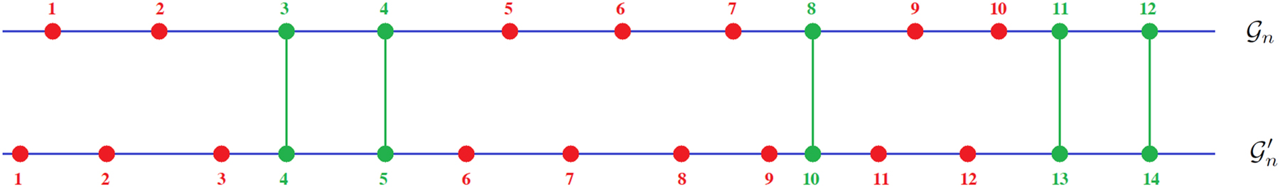
Illustration for the proof of Lemma 3.7. The dots on the first line are the points of
and
|i k − j k | ⩽ b n for all k = 1, …, a n . Indeed, if
and
From
It remains to prove that
Recall that, by assumption,
We consider two cases.
j ∈ J n . In this case, j = j k for some k = 1, …, a n and
(3.6)j ∉ J n . In this case, let j k , j k+1 ∈ J n be the two indices in J n surrounding j as in Figure 2. Note that j k may not exist if j is “too close” to the left boundary (as it would happen in Figure 2 if j were equal to 1, 2 or 3); in this situation, we have j k+1 = j 1 and we set by convention j k = j 0 = 0, i k = i 0 = 0,
j k < j < j k+1.
|j − j k | ⩽ b n . Indeed, looking at Figure 2 and keeping in mind our conventions for the left and right boundaries, we have
|i k+1 − i k | ⩽ b n + 1. Indeed, looking at Figure 2 and keeping in mind our conventions for the left and right boundaries, we have
Thus,
In conclusion, by combining the two considered cases, for all
which is a quantity independent of j and tending to 0 as n → ∞ (recall that b
n
= o(d
n
) and
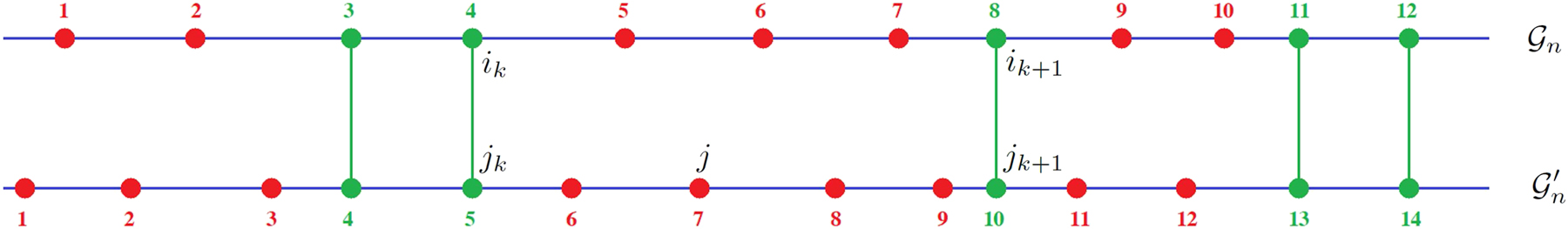
Illustration for the proof of Lemma 3.7.
3.4 Properties of continuous functions satisfying particular conditions
Lemma 3.8 highlights a property of continuous monotone functions on a compact interval. This property can be proved on the basis of the following more general results:
if
if
However, for the reader’s convenience, we include a direct proof of Lemma 3.8.
Lemma 3.8.
Let
Proof.
We prove the lemma under the assumption that f is strictly increasing on [a, b]; the proof in the case where f is strictly decreasing on [a, b] is completely analogous. Fix δ > 0. Since f is continuous and strictly increasing on [a, b], the function
Similarly, the function
If we set ɛ = min(ɛ +, ɛ −) > 0, then we see that
which is equivalent to
Thus, for every x ∈ [a + δ, b − δ] we have [f(x) − ɛ, f(x) + ɛ] ⊆ [f(x − δ), f(x + δ)] = f([x − δ, x + δ]), where the latter equality follows from the fact that f is continuous and monotone increasing. □
Lemma 3.9 shows that the preimage of any point through a continuous function
Lemma 3.9.
Let I be a bounded real interval and let
Proof.
For a given
Now, suppose by contradiction that f
−1(λ) is infinite for a certain
Corollary 3.1.
Let I be a bounded real interval and let
Proof.
Let a < b be the endpoints of the interval I and let a = η
0 < η
1 < … < η
ℓ
< η
ℓ+1 = b be the discontinuity points of f, to which we also add the boundary points η
0 = a and η
ℓ+1 = b. Note that the restriction
is finite by Lemma 3.9. □
3.5 Proof of Theorem 2.2
The last results we need to prove Theorem 2.2 are the following two technical lemmas. Lemma 3.10 provides a straightforward estimate of the largest number of points taken from a uniform grid that can lie in a fixed interval; the proof is left to the reader. Lemma 3.11 is a slight generalization of ref. [1], Ex. 3.3].
Lemma 3.10.
Let h > 0 and let
Lemma 3.11.
For every ɛ > 0, let
Proof.
Since q n (ɛ) → q(ɛ) for every ɛ > 0,
for ɛ = 1 there exists n 1 such that |q n (1) − q(1)| ⩽ 1 for n ⩾ n 1,
for
for
…
Define
ɛ n = 1 for n < n 2,
…
By construction, ɛ n → 0 and |q n (ɛ n ) − q(ɛ n )| ⩽ ɛ n for n⩾n 2, so |q n (ɛ n )| ⩽ |q(ɛ n )| + ɛ n for n⩾n 2 and q n (ɛ n ) → 0. □
Proof of Theorem 2.2.
Let θ
i,n
= a + i(b − a)/d
n
, i = 1, …, d
n
. It is clear that the grid
where for simplicity we have set
We show that
For every δ, ɛ ⩾ 0 and every n, we define the “bad” sets
We call them “bad” sets, because if
where
Now, let a = ξ
0 < ξ
1 < … < ξ
k
< ξ
k+1 = b be the local maximum points, local minimum points, and discontinuity points of f, to which we also add the boundary points ξ
0 = a and ξ
k+1 = b. For every j = 0, …, k, the function f is continuous on (ξ
j
, ξ
j+1) and has no local maximum/minimum points on (ξ
j
, ξ
j+1), so it is strictly monotone on (ξ
j
, ξ
j+1). Thus, by Lemma 3.8 applied to
Hence, for every δ > 0 there exists ɛ (δ) = min j=0,…,k ɛ (j,δ) > 0 such that
For every δ > 0, let n
δ
be such that ɛ
n
⩽ ɛ
(δ) for n ⩾ n
δ
. If n ⩾ n
δ
and i ∈ {1, …, d
n
} is an index such that
Hence,
where the latter inequality is due to Lemma 3.10. We can therefore choose, by Lemma 3.11, a sequence of positive numbers
To conclude the proof, let
The grid
3.6 Concatenation lemma
The following lemma is a plain consequence of Definition 1.1 and has often been used in the literature, but lucid statement and proof have never been provided. We therefore provide the details below.
Lemma 3.12
(concatenation lemma). Let
Proof.
The result follows from Definition 1.1, after observing that, for every
where in the second equality we have used the change of variable formula for the Lebesgue integral. □
3.7 Restriction operator and asymptotic spectral distribution of restricted matrix-sequences
For every n ⩾ 1, let Ξ
n
be the uniform grid in [0, 1] given by Ξ
n
= {i/(n + 1): i = 1, …, n}. If
Lemma 3.13.
Let Ω ⊆ [0, 1] be a regular set with μ
1(Ω) > 0, let
3.8 GLT sequences
Let
Lemma 3.14.
Let
The second property is reported in the next lemma [32], Th. 2].
Lemma 3.15.
Let
The third property is reported in the next lemma, which has never appeared in the literature.
Lemma 3.16
(splitting of GLT sequences formed by diagonal matrices). Let
Then
Proof.
Let Ω
j
= [(j − 1)/k, j/k] for j = 1, …, k, and fix j ∈ {1, …, k}. Since
Let
For every n, we have
where the last inequality is due to Lemma 3.10. Since L n,i /d n → 1/k as n → ∞ for every i = 1, …, k by assumption, we have
and so
□
3.9 Proof of Lemma 2.1
We have now collected all the ingredients to prove Lemma 2.1.
Proof of Lemma 2.1.
By Lemma 3.12, the hypothesis
By Lemma 3.15, there exists a sequence
By Lemma 3.16, we conclude that
Since
(this is proved by direct computation using the change of variable formula for the Lebesgue integral as in the proof of Lemma 3.12), the thesis is proved with
□
3.10 Proof of Lemma 2.2
In order to prove Lemma 2.2, we need some auxiliary results. The first result is reported in the next lemma [1], Th. 3.1].
Lemma 3.17.
If
where d n is the size of A n .
The second result is reported in the next lemma [1], Th. 3.2]. In what follows, the notation
Lemma 3.18.
Let
The third result is reported in the next lemma [1], Ex. 5.3].
Lemma 3.19.
Let
The last result is the following lemma of graph theory. In what follows, given a directed graph
Lemma 3.20.
Let X be a finite set, and let A
1, …, A
k
and B
1, …, B
k
be two partitions of X with |A
i
| = |B
i
| for every i = 1, …, k. Let
Proof.
Suppose by contradiction that (i, j) ∈ E but there is no directed path from j to i. Then, the sets of nodes
are disjoint. Moreover, there is no edge from N
j
to
where the last inequality follows by letting x vary in N
j
∪ {i} instead of V. We have thus obtained a contradiction, because
Proof of Lemma 2.2.
The hypotheses of Lemma 2.1 are satisfied with f
1, …, f
k
, Λ
n
as in the statement of Lemma 2.2 and with
The partition
For every j = 1, …, k, since
Note that the previous limit relation continues to hold if we replace L
n,j
with d
n
(because
then we have the following: for every n there exists some δ n tending to 0 as n → ∞ such that ɛ n ⩽ δ n and, for every j = 1, …, k,
We remark that, since
Now, fix n and take an element
(with i 0, …, i q+1 ∈ {1, …, k} and i 0, …, i q distinct) and corresponding elements
(with x 0, …, x q ∈ Λ n ) such that
As a consequence, we can produce a new partition
by removing x
s
from
hence
Therefore, if in analogy with (3.12) we define
then we have
where the latter equation is due to the fact that x = x
0 has been removed from
we have produced a new partition
with the same cardinalities
and with
We can now repeat the same procedure for another element
with the same cardinalities
and with corresponding “E-sets”
where E n,j is defined in analogy with (3.12) and (3.16) as follows:
We prove that the partition {Λ n,1, …, Λ n,k } satisfies the three properties required in the thesis of the lemma.
The partition {Λ n,1, …, Λ n,k } satisfies the first property by (3.17) and the third property by (3.18) and (3.19). It only remains to prove that {Λ n,1, …, Λ n,k } satisfies the second property. To this end, we note that the above procedure must be repeated at most a number N n of times equal to
because each time we apply the procedure, the union of the “E-sets” loses an element (the final equality in (3.20) is due to (3.13)). Moreover, each time we apply the procedure, the new partition
For example, the first time we apply the procedure, we obtain
So, after N n applications of the procedure, we obtain
Thus, for every j = 1, …, k, if we define D
n,j
as in the second property of the thesis of the lemma, the previous inequality implies that, after a suitable permutation of its diagonal elements, D
n,j
becomes equal to
3.11 Proof of Theorem 2.3
We have now collected all the ingredients to prove Theorem 2.3.
Proof of Theorem 2.3.
The theorem follows immediately from Lemma 2.2 and Corollary 2.1. Indeed, by Lemma 2.2, for every n there exists a partition {Λ n,1, …, Λ n,k } of Λ n such that, for every j = 1, …, k, the following properties hold:
Λ n,j ⊆ [inf[a,b] f j − δ n , sup[a,b] f j + δ n ] for some δ n → 0 as n → ∞.
By Corollary 2.1, for every j = 1, …, k and every a.u. grid
□
4 Numerical experiments
In this section, after recalling some properties of Toeplitz matrices, we illustrate our main results through numerical examples.
4.1 Preliminaries on Toeplitz matrices
It is not difficult to see that the conjugate transpose of T n (f) is given by
for every f ∈ L
1([−π, π]) and every n; see, e.g., [1], Sect. 6.2]. In particular, if f is real a.e., then
Theorem 4.1.
Let f ∈ L 1([−π, π]) be real and let m f = ess inf[−π,π] f and M f = ess sup[−π,π] f. Then, the following properties hold:
T n (f) is Hermitian and the eigenvalues of T n (f) lie in the interval [m f , M f ] for all n;
if f is not a.e. constant, then the eigenvalues of T n (f) lie in (m f , M f ) for all n;
4.2 Numerical examples
Example 4.1.
Let
For every a.u. grid
where τ n is a suitable permutation of {1, …, n}.
There exists an a.u. grid
where τ n is a suitable permutation of {1, …, n}.
The two previous assertions are actually well known in this case, because Λ n = {f(iπ/(n + 1)): i = 1, …, n}; see [33], Th. 2.4].
Example 4.2.
Let
and let Λ
n
= {λ
1,n
, …, λ
n,n
} be the multiset consisting of the eigenvalues of the Hermitian Toeplitz matrix T
n
(f). Figure 3 shows the graph of f over the interval [0, π]. By Theorem 4.1 and the fact that f is an even function, we have
where τ n is the permutation of {1, …, n} that sorts λ 1,n , …, λ n,n in increasing order (note that f|[0,π] is increasing). To provide numerical evidence of (4.2), in Table 1 we compute M n for increasing values of n in the case of the a.u. grid θ i,n = iπ/(n + 1), i = 1, …, n. We see from the table that M n → 0 as n → ∞, though the convergence is slow.
Now we observe that f|[0,π] and Λ
n
do not satisfy the assumptions of Theorem 2.2. Actually, they satisfy all the assumptions of Theorem 2.2 except the hypothesis that f has a finite number of local maximum/minimum points. Indeed, f is constant on [0, π/2] and so all points in [0, π/2) are both local maximum and local minimum points for f according to our Definition 2.1. We observe that, in fact, the thesis of Theorem 2.2 does not hold in this case, i.e., there is no a.u. grid
for a suitable permutation τ
n
of {1, …, n}. This is clear, because Λ
n
⊂ (1, 1 + π/2) and so any grid
![Figure 3:
Example 4.2: Graph on the interval [0, π] of the function f(θ) defined in (4.1).](/document/doi/10.1515/jnma-2023-0091/asset/graphic/j_jnum-2023-0091_fig_003.jpg)
Example 4.2: Graph on the interval [0, π] of the function f(θ) defined in (4.1).
Example 4.2: Computation of M n for increasing values of n.
| n | M n |
|---|---|
| 8 | 0.0851 |
| 16 | 0.0632 |
| 32 | 0.0454 |
| 64 | 0.0312 |
| 128 | 0.0206 |
| 256 | 0.0132 |
| 512 | 0.0082 |
| 1,024 | 0.0050 |
Example 4.3.
Let
and let Λ
n
= {λ
1,n
, …, λ
n,n
} be the multiset consisting of the eigenvalues of the Hermitian Toeplitz matrix T
n
(f). Figure 4 shows the graph of f over the interval [0, π]. By Theorem 4.1 and the fact that f is an even function, we have
For every a.u. grid
(4.4)where σ n and τ n are two permutations of {1, …, n} such that the vectors
There exists an a.u. grid
where τ n is a suitable permutation of {1, …, n}.
To provide numerical evidence of (4.4), in Table 2 we compute M n for increasing values of n in the case of the a.u. grid θ i,n = iπ/(n + 1), i = 1, …, n. We see from the table that M n → 0 as n → ∞, though the convergence is slow.
![Figure 4:
Example 4.3: Graph on the interval [0, π] of the function f(θ) defined in (4.3).](/document/doi/10.1515/jnma-2023-0091/asset/graphic/j_jnum-2023-0091_fig_004.jpg)
Example 4.3: Graph on the interval [0, π] of the function f(θ) defined in (4.3).
Example 4.3: Computation of M n for increasing values of n.
| n | M n |
|---|---|
| 8 | 0.7220 |
| 16 | 0.5625 |
| 32 | 0.4471 |
| 64 | 0.2956 |
| 128 | 0.1783 |
| 256 | 0.1096 |
| 512 | 0.0605 |
| 1,024 | 0.0373 |
Example 4.4.
Consider the following second-order differential problem:
where
where a
i
= a(x
i
) for all i in the real interval [0, n + 1]; see [1], Sect. 10.5.1] for more details. Let
where the latter equality follows from the continuity of f and the fact that the domain [0, 1] × [0, π] is not “too wild” (in particular, it is contained in the closure of its interior); see [1], Ex. 2.1].
Now, following the notations of Theorem 2.1, let
a
= (0, 0) and
b
= (1, π), so that [
a
,
b
] = [0, 1] × [0, π]. Assume that n is a perfect square, let
and let
where σ n and τ n are two permutations of {1, …, n} such that the vectors
are sorted in increasing order. To provide numerical evidence of (4.5), in Table 3 we compute M n for increasing values of n and different choices of a(x). In all cases, we see from the table that M n → 0 as n → ∞, though the convergence is slow.
Example 4.4: Computation of M n for increasing values of n and different choices of a(x).
| (a) a(x) = e−x | (b) a(x) = 2 + cos(3x) | (c) a(x) = x log(1 + x) | |||
|---|---|---|---|---|---|
| n | M n | n | M n | n | M n |
| 900 | 0.0684 | 900 | 0.1471 | 900 | 0.1240 |
| 1,600 | 0.0559 | 1,600 | 0.1132 | 1,600 | 0.0915 |
| 2,500 | 0.0473 | 2,500 | 0.0890 | 2,500 | 0.0717 |
| 3,600 | 0.0411 | 3,600 | 0.0738 | 3,600 | 0.0583 |
| 4,900 | 0.0364 | 4,900 | 0.0634 | 4,900 | 0.0497 |
| 6,400 | 0.0326 | 6,400 | 0.0558 | 6,400 | 0.0435 |
| 8,100 | 0.0296 | 8,100 | 0.0484 | 8,100 | 0.0383 |
| 10,000 | 0.0271 | 10,000 | 0.0436 | 10,000 | 0.0344 |
Example 4.5.
Consider the two-dimensional Poisson problem
In the isogeometric Galerkin discretization based on tensor-product biquadratic B-splines defined over the uniform grid i / n for i = 0, …, n and n = n (n) = (n, n), the computation of the numerical solution reduces to solving a linear system whose coefficient matrix is the symmetric n 2 × n 2 matrix given by
where ⊗ is the Kronecker tensor product and K n , M n are the symmetric n × n matrices given by
see [2], Sect. 7.6] for more details. Let
where
and let
for all n. Thus, Theorem 2.1 applies in this case. In fact, in view of the spectral decompositions obtained in ref. [35], Sect. 3.3], the eigenvalues of A n are exactly given by
where
n
=
n
(n) = (n, n) as above and
Example 4.6.
Consider the following second-order differential problem:
In the classical Galerkin method with basis functions given by the 2n − 1 B-splines of degree 2 and smoothness C
0([0, 1]) defined over the uniform knot sequence
see [22], Sect. 2.3.2] for more details. Let
and let Λ
n
= {λ
1,n
, …, λ
2n−1,n
} be the multiset consisting of the eigenvalues of A
n
(sorted in increasing order for later convenience). We know from refs. [5], Th. 6.5] and [22], Sect. 2.3.2] that
Figure 5 shows the graphs of the functions f 1,2(θ) and the set of eigenvalues Λ n for n = 20. The eigenvalues λ i,n , i = 1, …, 2n − 1, are positioned at iπ/n for i = 1, …, n and (i − n)π/n for i = n + 1, …, 2n − 1. Note that
From the figure, we may assume that the hypotheses of Theorem 2.3 are satisfied with the partition
if
(4.8)(4.9)
Actually, we can say more than (4.8) and (4.9). Indeed, numerical experiments reveal that M n,1 = M n,2 = 0 for all n if we choose the a.u. grids suggested by Figure 5, i.e., θ i,n = iπ/n, i = 1, …, n, and ϑ i,n = iπ/n, i = 1, …, n − 1. In other words, the eigenvalues of A n are explicitly given by
We refer the reader to Appendix A for further explicit formulas for the eigenvalues of B-spline Galerkin discretization matrices. These formulas have been obtained through numerical experiments and provide further confirmations of Theorem 2.3.
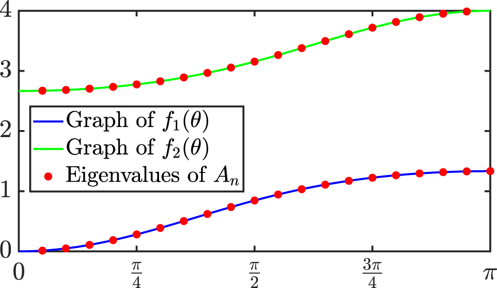
Example 4.6: Graphs of the functions f 1,2(θ) in (4.6)–(4.7) and set of eigenvalues Λ n for n = 20.
5 Conclusions
We have provided new insights into the notion of asymptotic (spectral) distribution by extending previous results due to Bogoya, Böttcher, Grudsky, and Maximenko [25], [26]. In particular, using the concept of monotone rearrangement (quantile function) and matrix analysis arguments from the theory of GLT sequences, we have shown that, under suitable assumptions, if the asymptotic distribution of a sequence of multisets
We conclude this paper with a remark. The notion of asymptotic distribution given in Definition 1.2 is deeply connected with the notion of vague convergence of probability measures, which is also referred to as convergence in distribution in ref. [26]. More precisely, as shown in ref. [32]:
if
where δ z is the Dirac probability measure such that δ z (E) = 1 if z ∈ E and δ z (E) = 0 otherwise;
if f is as in Definition 1.2 with k = 1, then we can associate with f a uniquely determined probability measure μ f on
The asymptotic distribution relation
can therefore be rewritten as
which is equivalent to saying that
Acknowledgments
Giovanni Barbarino, Carlo Garoni and Stefano Serra-Capizzano are members of the Research Group GNCS (Gruppo Nazionale per il Calcolo Scientifico) of INdAM (Istituto Nazionale di Alta Matematica).
-
Research ethics: Not applicable.
-
Informed consent: Not applicable.
-
Author contributions: All authors have accepted responsibility for the entire content of this manuscript and approved its submission. Giovanni Barbarino provided the proofs of the main results of the paper. Carlo Garoni revised/fine-tuned/extended these proofs and wrote the paper. Sven-Erik Ekström, Stefano Serra-Capizzano and Paris Vassalos had the idea of this paper and wrote the original version of the manuscript. Sven-Erik Ekström and David Meadon performed the numerical experiments in Section 4 and Appendix A.
-
Use of Large Language Models, AI and Machine Learning Tools: None declared.
-
Conflict of interest: The authors state no conflict of interest.
-
Research funding: Giovanni Barbarino was supported by the Alfred Kordelinin Säätiö Grant 210122 and the European Research Council (ERC) Consolidator Grant 101085607 through the Project eLinoR. Carlo Garoni was supported by an INdAM-GNCS Project (CUP E53C22001930001) and by the Department of Mathematics of the University of Rome Tor Vergata through the MUR Excellence Department Project MatMod@TOV (CUP E83C23000330006) and the Project RICH_GLT (CUP E83C22001650005). David Meadon was funded by the Centre for Interdisciplinary Mathematics (CIM) at Uppsala University. Stefano Serra-Capizzano was funded by the PRIN-PNRR (Piano Nazionale di Ripresa e Resilienza) Project MATHPROCULT (MATHematical tools for predictive maintenance and PROtection of CULTural heritage, Code P20228HZWR, CUP J53D23003780006) and by the European High-Performance Computing Joint Undertaking (JU) under Grant Agreement 955701. The JU receives support from the European Union's Horizon 2020 Research and Innovation Programme and Belgium, France, Germany, Switzerland. Stefano Serra-Capizzano is also grateful to the Theory, Economics and Systems Laboratory (TESLAB) of the Department of Computer Science at the Athens University of Economics and Business for providing financial support.
-
Data availability: Not applicable.
Appendix A: Formulas for the eigenvalues of B-spline Galerkin discretization matrices
Consider the following second-order differential eigenvalue problem:
Let p ⩾ 1 and 0 ⩽ k ⩽ p − 1. In the classical Galerkin method with basis functions given by the n(p − k) + k − 1 B-splines B 2,p,k , …, B n(p−k)+k,p,k of degree p and smoothness C k ([0, 1]) defined over the uniform knot sequence
and vanishing at the boundary points x = 0 and x = 1, the computation of the numerical solution reduces to solving a linear system whose coefficient matrix is the (n(p − k) + k − 1) × (n(p − k) + k − 1) matrix given by
where K n,p,k , M n,p,k are the symmetric positive definite matrices given by
see [22], Sect. 2.5] for more details. We remark that, for p = 2 and k = 1, the matrix n −1 K n,2,1 coincides with the matrix A n of Example 4.6. As proved in ref. [5], Th. 6.17], we have
where:
the functions
the blocks
the functions
We remark that, for every θ ∈ [0, π], the matrix f p,k (θ) is Hermitian positive semidefinite and the matrix h p,k (θ) is Hermitian positive definite; see [22], Rem. 2.1]. The following Maple worksheet computes f p,k (θ) and h p,k (θ) for the input pair p, k defined at the beginning. Here, we have chosen p = 2 and k = 0 for comparison with Example 4.6.
| >p ≔ 2: k ≔ 0: |
|
|
| > with(CurveFitting): with(LinearAlgebra): |
|
|
| > # Construction of the reference B-splines β 1,p,k , …, β p−k,p,k |
| > β ≔ [ ]: |
|
|
|
|
|
|
| > # Derivatives of the reference B-splines β 1,p,k , …, β p−k,p,k |
| > D_β ≔ simplify(diff(β, t)): |
|
|
| > Kblocks≔ [ ]: Mblocks≔ [ ]: |
|
|
|
|
|
|
|
|
|
|
|
|
|
|
| > # Construction of the functions f = f p,k and h = h p,k |
| > f(θ) ≔ Kblocks[1]: h(θ) ≔ Mblocks[1]: |
|
|
|
|
|
|
|
|
|
|
In Theorems A.1–A.3, we report the formulas for the eigenvalues of the matrices n −1 K n,p,k , nM n,p,k , n −2 L n,p,k that we obtained through high-precision numerical computations performed in Julia, using an accuracy of at least 100 decimal digits. In what follows, for every θ ∈ [0, π] and every j = 1, …, p − k, we define λ j (f p,k (θ)) (resp., λ j (h p,k (θ)), λ j (e p,k (θ))) as the jth eigenvalue of f p,k (θ) (resp., h p,k (θ), e p,k (θ)) according to the increasing ordering:
Moreover, for every n ⩾ 1, we define the uniform grids
Theorem A.1.
Let 1 ⩽ p ⩽ 100 and 0 ⩽ k ⩽ min(1, p − 1). Then, for every n = 1, …, 100, the eigenvalues of n −1 K n,p,k are given by
where the grid
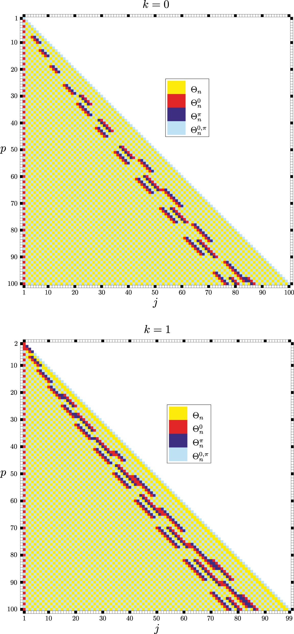
Grid
Conjecture A.1.
Theorem A.1 continues to hold if we replace “for every n = 1, …, 100” with “for every n ⩾ 1”.
To simplify the statement of Theorem A.2, we define the integer sequence
The sequence
It is not difficult to check that
Theorem A.2.
Let 1 ⩽ p ⩽ 100 and 0 ⩽ k ⩽ min(1, p − 1). Then, for every n = 1, …, 100, the eigenvalues of nM n,p,k are given by
where the grid
Conjecture A.2.
Theorem A.2 continues to hold if we replace “1 ⩽ p ⩽ 100” with “p ⩾ 1” and “for every n = 1, …, 100” with “for every n ⩾ 1”.
Theorem A.3.
Let 1 ⩽ p ⩽ 100 and 0 ⩽ k ⩽ min(1, p − 1). Then, for every n = 1, …, 20, the eigenvalues of n −2 L n,p,k are given by
where the grid
Conjecture A.3.
Theorem A.3 continues to hold if we replace “1 ⩽ p ⩽ 100” with “p ⩾ 1” and “for every n = 1, …, 20” with “for every n ⩾ 1”.
References
[1] C. Garoni and S. Serra-Capizzano, Generalized Locally Toeplitz Sequences: Theory and Applications, vol. I, Cham, Springer, 2017.10.1007/978-3-319-53679-8Suche in Google Scholar
[2] C. Garoni and S. Serra-Capizzano, Generalized Locally Toeplitz Sequences: Theory and Applications, vol. II, Cham, Springer, 2018.10.1007/978-3-030-02233-4Suche in Google Scholar
[3] G. Barbarino, “A systematic approach to reduced GLT,” BIT Numer. Math., vol. 62, pp. 681–743, 2022, https://doi.org/10.1007/s10543-021-00896-7.Suche in Google Scholar
[4] G. Barbarino, C. Garoni, M. Mazza, and S. Serra-Capizzano, “Rectangular GLT sequences,” Electron. Trans. Numer. Anal., vol. 55, pp. 585–617, 2022, https://doi.org/10.1553/etna_vol55s585.Suche in Google Scholar
[5] G. Barbarino, C. Garoni, and S. Serra-Capizzano, “Block generalized locally Toeplitz sequences: theory and applications in the unidimensional case,” Electron. Trans. Numer. Anal., vol. 53, pp. 28–112, 2020, https://doi.org/10.1553/etna_vol53s28.Suche in Google Scholar
[6] G. Barbarino, C. Garoni, and S. Serra-Capizzano, “Block generalized locally Toeplitz sequences: theory and applications in the multidimensional case,” Electron. Trans. Numer. Anal., vol. 53, pp. 113–216, 2020, https://doi.org/10.1553/etna_vol53s113.Suche in Google Scholar
[7] A. Böttcher, C. Garoni, and S. Serra-Capizzano, “Exploration of Toeplitz-like matrices with unbounded symbols is not a purely academic journey,” Sb. Math., vol. 208, pp. 1602–1627, 2017, https://doi.org/10.1070/sm8823.Suche in Google Scholar
[8] U. Grenander and G. Szegő, Toeplitz Forms and Their Applications, 2nd ed. New York, AMS Chelsea Publishing, 1984.Suche in Google Scholar
[9] F. Avram, “On bilinear forms in Gaussian random variables and Toeplitz matrices,” Probab. Theory Relat. Fields, vol. 79, pp. 37–45, 1988, https://doi.org/10.1007/bf00319101.Suche in Google Scholar
[10] S. V. Parter, “On the distribution of the singular values of Toeplitz matrices,” Linear Algebra Appl., vol. 80, pp. 115–130, 1986, https://doi.org/10.1016/0024-3795(86)90280-6.Suche in Google Scholar
[11] E. E. Tyrtyshnikov, “A unifying approach to some old and new theorems on distribution and clustering,” Linear Algebra Appl., vol. 232, pp. 1–43, 1996, https://doi.org/10.1016/0024-3795(94)00025-5.Suche in Google Scholar
[12] E. E. Tyrtyshnikov and N. L. Zamarashkin, “Spectra of multilevel Toeplitz matrices: advanced theory via simple matrix relationships,” Linear Algebra Appl., vol. 270, pp. 15–27, 1998, https://doi.org/10.1016/s0024-3795(97)80001-8.Suche in Google Scholar
[13] N. L. Zamarashkin and E. E. Tyrtyshnikov, “Distribution of eigenvalues and singular values of Toeplitz matrices under weakened conditions on the generating function,” Sb. Math., vol. 188, pp. 1191–1201, 1997, https://doi.org/10.1070/sm1997v188n08abeh000251.Suche in Google Scholar
[14] P. Tilli, “A note on the spectral distribution of Toeplitz matrices,” Linear Multilinear Algebra, vol. 45, pp. 147–159, 1998, https://doi.org/10.1080/03081089808818584.Suche in Google Scholar
[15] P. Tilli, “Some results on complex Toeplitz eigenvalues,” J. Math. Anal. Appl., vol. 239, pp. 390–401, 1999, https://doi.org/10.1006/jmaa.1999.6572.Suche in Google Scholar
[16] A. Böttcher and B. Silbermann, Introduction to Large Truncated Toeplitz Matrices, New York, Springer, 1999.10.1007/978-1-4612-1426-7Suche in Google Scholar
[17] S. Serra-Capizzano, “Generalized locally Toeplitz sequences: spectral analysis and applications to discretized partial differential equations,” Linear Algebra Appl., vol. 366, pp. 371–402, 2003, https://doi.org/10.1016/s0024-3795(02)00504-9.Suche in Google Scholar
[18] S. Serra-Capizzano, “The GLT class as a generalized Fourier analysis and applications,” Linear Algebra Appl., vol. 419, pp. 180–233, 2006, https://doi.org/10.1016/j.laa.2006.04.012.Suche in Google Scholar
[19] P. Tilli, “Locally Toeplitz sequences: spectral properties and applications,” Linear Algebra Appl., vol. 278, pp. 91–120, 1998, https://doi.org/10.1016/s0024-3795(97)10079-9.Suche in Google Scholar
[20] D. Bianchi, “Analysis of the spectral symbol associated to discretization schemes of linear self-adjoint differential operators,” Calcolo, vol. 58, 2021, Art. no. 38, https://doi.org/10.1007/s10092-021-00426-5.Suche in Google Scholar
[21] D. Bianchi and S. Serra-Capizzano, “Spectral analysis of finite-dimensional approximations of 1d waves in non-uniform grids,” Calcolo, vol. 55, 2018, Art. no. 47, https://doi.org/10.1007/s10092-018-0288-x.Suche in Google Scholar
[22] C. Garoni, H. Speleers, S.-E. Ekström, A. Reali, S. Serra-Capizzano, and T. J. R. Hughes, “Symbol-based analysis of finite element and isogeometric B-spline discretizations of eigenvalue problems: exposition and review,” Arch. Comput. Methods Eng., vol. 26, pp. 1639–1690, 2019.10.1007/s11831-018-9295-ySuche in Google Scholar
[23] B. Beckermann and A. B. J. Kuijlaars, “Superlinear convergence of conjugate gradients,” SIAM J. Numer. Anal., vol. 39, pp. 300–329, 2001, https://doi.org/10.1137/s0036142999363188.Suche in Google Scholar
[24] A. B. J. Kuijlaars, “Convergence analysis of Krylov subspace iterations with methods from potential theory,” SIAM Rev., vol. 48, pp. 3–40, 2006, https://doi.org/10.1137/s0036144504445376.Suche in Google Scholar
[25] J. M. Bogoya, A. Böttcher, S. M. Grudsky, and E. A. Maximenko, “Maximum norm versions of the Szegő and Avram–Parter theorems for Toeplitz matrices,” J. Approx. Theory, vol. 196, pp. 79–100, 2015.10.1016/j.jat.2015.03.003Suche in Google Scholar
[26] J. M. Bogoya, A. Böttcher, and E. A. Maximenko, “From convergence in distribution to uniform convergence,” Bol. Soc. Mat. Mex., vol. 22, pp. 695–710, 2016, https://doi.org/10.1007/s40590-016-0105-y.Suche in Google Scholar
[27] B. Fristedt and L. Gray, A Modern Approach to Probability Theory, Boston, Birkhäuser, 1997.10.1007/978-1-4899-2837-5Suche in Google Scholar
[28] W. Rudin, Principles of Mathematical Analysis, 3rd ed. New York, McGraw-Hill, 1976.Suche in Google Scholar
[29] G. Barbarino, D. Bianchi, and C. Garoni, “Constructive approach to the monotone rearrangement of functions,” Expo. Math., vol. 40, pp. 155–175, 2022, https://doi.org/10.1016/j.exmath.2021.10.004.Suche in Google Scholar
[30] G. Pólya and G. Szegő, Problems and Theorems in Analysis I. Series. Integral Calculus. Theory of Functions, Berlin–Heidelberg, Springer, 1998.10.1007/978-3-642-61905-2Suche in Google Scholar
[31] R. Bhatia, Matrix Analysis, New York, Springer, 1997.10.1007/978-1-4612-0653-8Suche in Google Scholar
[32] G. Barbarino, “Spectral measures,” in Structured Matrices in Numerical Linear Algebra: Analysis, Algorithms and Applications, Springer INdAM Series, vol. 30, Cham, Springer, 2019, pp. 1–24.10.1007/978-3-030-04088-8_1Suche in Google Scholar
[33] A. Böttcher and S. M. Grudsky, Spectral Properties of Banded Toeplitz Matrices, Philadelphia, SIAM, 2005.10.1137/1.9780898717853Suche in Google Scholar
[34] D. Noutsos, S. Serra-Capizzano, and P. Vassalos, “The conditioning of FD matrix sequences coming from semi-elliptic differential equations,” Linear Algebra Appl., vol. 428, pp. 600–624, 2008, https://doi.org/10.1016/j.laa.2007.08.008.Suche in Google Scholar
[35] S.-E. Ekström, I. Furci, C. Garoni, C. Manni, S. Serra-Capizzano, and H. Speleers, “Are the eigenvalues of the B-spline isogeometric analysis approximation of −Δu = λu known in almost closed form?” Numer. Linear Algebra Appl., vol. 25, 2018, Art. no. e2198.10.1002/nla.2198Suche in Google Scholar
[36] A. Klenke, Probability Theory: A Comprehensive Course, London, Springer, 2008.Suche in Google Scholar
© 2025 the author(s), published by De Gruyter, Berlin/Boston
This work is licensed under the Creative Commons Attribution 4.0 International License.