Generalized energy-conserving dissipative particle dynamics with mass transfer: coupling between energy and mass exchange
-
Giuseppe Colella
 ,
Allan D. Mackie
,
James P. Larentzos
,
John K. Brennan
,
Martin Lísal
and
Josep Bonet Avalos
,
Allan D. Mackie
,
James P. Larentzos
,
John K. Brennan
,
Martin Lísal
and
Josep Bonet Avalos


Abstract
The complete description of energy and material transport within the Generalized energy-conserving dissipative particle dynamics with mass transfer (GenDPDE-M) methodology is presented. In particular, the dynamic coupling between mass and energy is incorporated into the GenDPDE-M, which was previously introduced with dynamically decoupled fluxes (J. Bonet Avalos et al., J. Chem. Theory Comput., 18 (12): 7639–7652, 2022). From a theoretical perspective, we have derived the appropriate Fluctuation-Dissipation theorems along with Onsager’s reciprocal relations, suitable for mesoscale models featuring this coupling. Equilibrium and non-equilibrium simulations are performed to demonstrate the internal thermodynamic consistency of the method, as well as the ability to capture the Ludwig–Soret effect, and tune its strength through the mesoscopic parameters. In view of the completeness of the presented approach, GenDPDE-M is the most general Lagrangian method to deal with complex fluids and systems at the mesoscale, where thermal agitation is relevant.
1 Introduction
The macroscopic behavior and properties of complex systems such as biological matter, composite materials or complex fluids, depend on the dynamics of phenomena occurring at the micro- and mesoscale. For such systems, the coupling between energy and mass transport is important for the understanding of several physicochemical scenarios, ranging from molecular motors to heterogeneous catalysis, with many important applications, e.g., in most chemical engineering processes. While atomistic modeling and simulation is a valuable tool, the computational cost of its application to such complex systems, whose characteristic temporal and spatial breadths are typically large compared to molecular dimensions, is often prohibitive. Coarse-grain (CG) modeling has become a vital alternative in cases where atomistic approaches are limiting or impractical. Among the wide variety of CG methods developed over the last decades, Dissipative Particle Dynamics (DPD) [1] has become a popular tool. Standard DPD is a Lagrangian, Galilean-invariant method whose dynamics conserves the total momentum and number of particles. As a consequence, the associated fields satisfy the corresponding hydrodynamic equations in the hydrodynamic limit [2], namely, Navier–Stokes and continuity equations [3]. In the standard DPD approach, the total force acting on a CG particle takes into account conservative as well as dissipative forces. The dissipation enters into the description through the CGing, due to the coupling between the resolved and CG degrees of freedom. Wherever dissipation occurs, implicitly there is a random contribution due to the thermal agitation of the non-resolved degrees of freedom [2]. In the DPD method, these contributions are added in the form of Langevin-like random forces between particles, which still preserve the Galilean invariance of the model. The dissipative friction force depends on both the positions and linearly on the velocity difference between the particles, through a coefficient that determines the strength of the force. The random contribution, on the other hand, is characterized by a Gaussian distribution and an amplitude that is related to the strength of the friction force through the corresponding Fluctuation-Dissipation (FD) theorem. In standard DPD method, the intensity of the random force depends on the system temperature T as a parameter [4]. Therefore, DPD is by construction isothermal and as a consequence heat flow cannot be modeled. An extension of the original DPD method was developed afterwards to include energy conservation, referred to as DPD with Energy Conservation (DPDE) [5], [6]. In DPDE, particles carry internal energy, stored into the CG degrees of freedom, and exhibit a particle temperature involved in the interparticle heat exchange. Since their development, both DPD and DPDE have been increasingly applied in different research areas [7], [8], [9], [10]. Recently, the Generalized Energy-Conserving DPD (GenDPDE) method [11], [12] has been proposed as a further extension of DPDE. The fundamental idea behind GenDPDE is the introduction of a particle fluctuating thermodynamics, which allows for a consistent definition of many-body forces that can depend on the particle temperature and particle density, unlike previous many-body DPD models in which the forces depend only on the local density [13], [14], [15], [16], [17], [18], [19], [20], or even parametrically on the system temperature [21]. More specifically, within the GenDPDE framework the force exerted by each mesoparticle can be related to its internal pressure, which depends on the particle volume and temperature through a particle Equation of State (EoS). In this way, the GenDPDE method permits the definition of temperature- and density-dependent forces, which are relevant for modeling non-equilibrium phenomena occurring in systems undergoing, e.g., chemical reactions [22] or shock compressions [23].
The concept of a fluctuating particle thermodynamics readily allowed for an extension of the GenDPDE framework to also include chemical composition into the description of the particle thermodynamic state. This extension is referred to as GenDPDE-M [24], [25]. Analogous to the heat flux in GenDPDE, in the new framework matter can be exchanged with neighboring mesoparticles through diffusive fluxes. However, GenDPDE-M in its first formulation (see the aforementioned references) disregarded any dynamic coupling between energy and material transport, which is in reality present in many relevant physical scenarios. Therefore, the introduction of the dynamic coupling between energy and mass fluxes presented in this work is a critical extension of GenDPDE-M.
In this article, we develop the theoretical framework to account for the coupling between mass and energy transport at the mesoscale. The outcome of our work is, therefore, a GenDPDE-M method that is complete and allows general, complex cases, involving momentum, energy and material transports, to be addressed in a unified way. Thus, within the complete GenDPDE-M method, phenomena such as the Ludwig–Soret effect can be properly modeled.
The manuscript is organized as follows. In Section 2, we review the theoretical framework based on the definition of the heat and diffusive fluxes along the lines of classical Onsager’s non-equilibrium thermodynamics [26], formulated at the mesoscale, where thermal agitation is relevant. We derive Langevin equations for the coupled energy and mass transfers to account for the thermal fluctuations. We highlight the key role of Detailed Balance (DB) in consistently formulating the fluctuating dynamics of complex CG systems. We show that DB not only sets the amplitude of the random contributions through FD relations, but also imposes the validity of Onsager’s reciprocal relations (ORR) at the mesoscopic level. We then introduce the van der Waals (vdW) particle thermodynamic model as a case study, which is used in both equilibrium and non-equilibrium simulations. In Section 3, we provide the computational details regarding our GenDPDE-M simulations. In Section 4, we present data obtained from equilibrium and non-equilibrium simulations. From these simulations, we show the consistency of the fluctuating local thermodynamic description, when coupling between mass and energy is present. Moreover, non-equilibrium simulations results are shown in which the dependency of the Ludwig–Soret effect on the strength of the mesoscopic coupling is discussed, along with the impact of the latter on the thermal conductivity of the system. Finally, Section 5 provides conclusions and future outlooks regarding GenDPDE-M.
2 Theoretical framework
In the general GenDPDE-M framework [24], [25], mesoparticles are regarded as property carriers whose state and dynamics are ultimately inherited from an existing underlying physical system. The latter can be regarded as being described by a classical Hamiltonian, with time-reversible trajectories, which ensures that an equilibrium probability distribution function exists and that DB is satisfied. The mesoscopic state variables are then a collection of surviving variables resulting from the CG process. Due to the elimination of internal degrees of freedom (non-surviving variables), the mesoscopic state variables can then be treated in a manner analogous to macroscopic Thermodynamics. For a simple multicomponent system, these surviving variables are the mesoparticle mass, m
i
, position, r
i
, momentum, p
i
, internal energy, u
i
, number density, n
i
(representative of the mesoparticle volume), and chemical composition. The dependence of the particle state on the chemical composition was introduced in the formulation of GenDPDE-M to incorporate material exchange into the GenDPDE framework [11], [12]. To describe composition, let us assume that the underlying physical system contains a number N
s
of different chemical species, each denoted by α and having a molecular mass
It is very important to realize that a given extensive property should be specified for each mesoparticle, to characterize its size. Without loss of generality, we fix the total mesoparticle mass
due to the constant mass constraint. Here,
In the following, we formulate heat and diffusive fluxes with coupling between them, which go beyond the initial approach presented in Refs. [24], [25]. We start by introducing, in Section 2.1, the concept of the particle fluctuating thermodynamics while the particles are kept at rest, for simplicity. We further outline the central object of the mesoscale thermodynamic description, i.e., the probability distributions for the state variables. In Section 2.2, we introduce the heat and diffusive fluxes, using Onsager’s formulation of non-equilibrium processes at the mesoscopic level [26], [28], since particles at rest can still exchange energy and mass due to these fluxes. We then provide explicit expressions for the general relations between the heat and diffusive fluxes with the corresponding thermodynamic forces, together with the associated random contributions, in Section 2.3. Finally, we derive the complete Equations-of-Motion (EoM) for the system of moving particles, which exchange energy and matter (Section 2.4). For completeness, in Section 2.5 we provide an example of a thermodynamic model for the mesoparticles, which is used in the simulations.
2.1 Probability distribution and intensive variables
For simplicity and clarity, but without loss of generality, let us consider mesoparticles with their positions fixed in space. Moreover, we restrain the discussion to binary mixtures (N s = 2). Although the generalization to multicomponent systems is straightforward, it requires quite a lengthy algebraic treatment [27].
The state of a static mesoparticle is defined by specifying its energetic content u
i
and the mass of the A-component
Following the analysis in Refs. [11], [12], the canonical equilibrium probability distribution for a system of N static mesoparticles with an embedded binary mixture is given by
where
In Eq. (3) we have explicitly assumed that the independent variables are the particles energies, u
i
, and the mass of species A,
which is a definition of the bare intensive variables,
where
It is important to realize that these intensive variables are estimators of the ensemble temperature and chemical potential, due to the fact that their equilibrium average yields [12],
where the macroscopic exchange chemical potential is defined as
According to Refs. [11], [12], Eq. (9) cannot be trivially inverted to express u
i
as a function of
where we have introduced s i as the so-called dressed particle entropy, related to the bare particle entropy by
with the Jacobian,
From Eq. (13), the relationship between the bare and dressed temperatures follows (see Eq. (17) of Ref. [12]),
Therefore, the thermodynamic relationship in Eq. (9) transforms into
where
The dressed variables are different estimators of the ensemble properties, i.e.,
Notice that the difference between dressed and bare variables is of the order of magnitude of the fluctuations, which should vanish with the size of the mesoparticles as k B /C V → 0, with C V being the mesoparticle heat capacity. In what follows, we require both the dressed and bare representations of the variables.
2.2 Heat and diffusive fluxes
From the exponent on the right-hand side of Eq. (3), we identify the free energy functional of the system, namely
Notice that this functional corresponds to the canonical ensemble and contains information about reservoir properties, i.e., the temperature T, which differs from the fluctuating particle temperature θ. In this form, we have arbitrarily chosen u
i
and
where the dot represents time-differentiation. Thus,
The equivalence of such statement and the traditional positiveness of the entropy production has been shown in Ref. [12]. Here, we will proceed straightforwardly from Eq. (22). As the independent variables are u i and m i , from Eq. (9), we can write
Thus,
The conserved quantities u i and m i follow some dynamic equations, which we aim at deriving eventually. On the one hand, the First Law of Thermodynamics also holds at the mesoscopic level,
where q i and W i are, respectively, the total heat transferred by mesoparticle i and the work done on mesoparticle i by the mechanical forces. Hence,
Since the mesoparticles are static, no mechanical work is exerted and, as a consequence,
namely, the irreversible energy exchange produced between particles is due to the exchange of mesoscopic heat. On the other hand, we can similarly assume that the irreversible material exchanges between particles are due to pairwise diffusive fluxes, i.e.,
The interparticle fluxes satisfy
To develop this equation further, we can first separate the summation over j ≠ i into two contributions, namely, j < i and j > i. Second, focusing on the second contribution, we can change the order of summation in such a way that ∑
i,j>i
… = ∑
j,i<j
…. Third, we can re-label the dummy indices i ↔ j and use the change of sign of
As the inequality must be satisfied irrespective of the number of pairs, we arrive to a more restrictive condition for every pair, i.e.,
From Eq. (31), we can identify the thermodynamic forces as
Notice that the thermodynamic forces are defined in terms of the bare intensive variables. Furthermore, from Eqs. (10) and (11) we can see that their equilibrium average exactly vanishes.
According to Onsager’s linear non-equilibrium thermodynamics [26], the heat and diffusive fluxes are defined as linear combinations of the thermodynamic forces sharing the same tensorial nature (Curie’s principle), which turns Eq. (31) into a quadratic expression in terms of the Y ij ’s. The implications of the inequality in Eq. (31) will be the subject of a later analysis. For our example, we thus write,
where
As a concluding remark, we comment on the usual distinction between the heat flux and measurable heat flux in the literature (see, e.g., [26], [30]). Theoretically, this distinction is related to what one would measure in a temperature gradient subject to the condition
where h α is the enthalpy per unit of mass of species α. Then, in classical non-equilibrium thermodynamics, from the entropy production equation it follows that the measurable heat flux can be defined as,
However, Eqs. (36) and (37) are only valid at the macroscopic level, i.e., with regards to the overall behavior of the ensemble of mesoparticles, independently of the form of Eqs. (34) and (35). For their validity, it is required that the spatial differences in the thermodynamic intensive variables are sufficiently small so that only the linear terms need to be retained, in view of Eq. (36). In Appendix A we show that the distinction between heat flux and a measurable counterpart at the level of the mesoparticles cannot be made. Only, if additional conditions on the size of the differences between particle temperatures apply, one can define a
2.3 Dynamics of energy and mass exchange of static mesoparticles
To the form given in Eqs. (34) and (35) for the systematic component of the dynamics, following the general GenDPDE-M scheme of Refs. [24], [25], we now add the effect of the thermal agitation through random fluxes, in the spirit of the so-called fluctuating hydrodynamics of Landau and Lifshitz [3]. We thus propose the complete EoM for static mesoparticles in a discrete form,
In Eqs. (38) and (39), prime and non-prime variables refer to the time t + δt and t, respectively; δt is the timestep, and
where
with
The coefficients
as m i is kept constant in GenDPDE-M. The EoM in Eqs. (38) and (39) can be written in a more compact form using matrix notation, i.e.,
where we have defined the vectors for the mesoscopic state, x i , thermodynamic forces, Y ij , and random contributions, Ω ij , as
together with the matrices of Onsager’s phenomenological coefficients, L ij , and the amplitudes of the random contributions, σ ij , according to
The mesoscopic transport coefficients in L ij and the amplitudes of the random terms in σ ij are linked together by the general FD theorem,
which is derived in Appendix B. In Eq. (49), the superscript T represents the transposed matrix. Moreover, in Appendix C we demonstrate that the ORR are also a consequence of DB, which implies that
For a binary mixture, this simply reduces to
Due to this symmetry, Eq. (49) implies that
where we introduced more natural notation for the coefficients, namely,
Here, κ ij can be regarded as the mesoscopic thermal conductivity coefficient, while Ð ij would be the mesoscopic Maxwell–Stefan diffusion coefficient [27]. Next, for convenience, we introduce the positive-definite coupling constants k u and k m from the relations,
Equation (52) thus become
These equations then can be solved to find the parameters involved in the coupling dynamics, i.e.,
Moreover, the cross-coefficient takes the form,
It is important to note that the amplitudes of the random terms are not unequivocally determined by simply fixing κ
ij
, Ð
ij
and
Next, in view of Eq. (31), Onsager’s coefficients must satisfy the following sign conditions,
which imply that κ ij > 0 and Ð ij > 0. In addition, from Eqs. (55) and (56) it also follows that k u > 0 and k m > 0. Moreover, from Eq. (63) we also find that the coupling constants are subject to the following inequality,
Combining Eq. (64) with the definitions of the amplitudes of the random terms, Eqs. (55), (56), (58), and (59), we arrive at the identification of the physically acceptable bounds for the coupling constants, namely,
The choice k
u
= k
m
implies that
2.4 The equations of motion
The dynamics of heat and mass transport, Eq. (46), with the corresponding FD relations, expressed in Eqs. (55), (56), (58) and (59), can be easily incorporated into the mechanical motion of a system of moving mesoparticles with an embedded binary mixture, because of our choice of constant mass (cf. Eq. (1)). The equilibrium distribution for the complete set of variables is the extension of Eq. (3) with the energy due to the mechanical degrees of freedom, i.e.,
where the functional form of
where w
ij
≡ w(r
ij
) is a smooth, monotonically decreasing (dw
ij
/dr
ij
< 0), non-negative, spherically symmetric weighting function. It vanishes for an interparticle distance, r
ij
≡ |r
i
− r
j
|, such that r
ij
≥ R
cut, where R
cut is the cut-off range. Unlike the other weighting functions defined in this work, w
ij
is normalized so that
Due to the spatial motion of the particles, here we have to explicitly take into account that the dissipative parameters are space-dependent, i.e.,
where ω
u
(r
ij
) and ω
m
(r
ij
) are smooth, monotonically decreasing, non-negative, and spherically symmetric weighting functions. They vanish for
where
As the positions are slow variables compared to u
i
,
The EoM for N mesoparticles in the coupled GenDPDE-M method are identical to those of Ref. [24], i.e.,
The dynamic coupling between mass and energy transport is taken into account through the form of the heat and mass fluxes, given by Eqs. (34) and (35), together with the random fluxes, Eqs. (40) and (41). For completeness, in Eqs. (74) and (75),
is the conservative force between a pair of mesoparticles i and j, where π i the particle pressure that follows from the free energy of the EoS for the mesoparticle. Note that the particle pressure will contribute to the overall system pressure as an excess pressure, as there is always an ideal contribution due to the thermal agitation of the mesoparticles. This point is important when defining the particle EoS targeting a given specific macroscopic thermodynamic behavior. In Eq. (78), e ij ≡ r ij /r ij . Further, the friction force takes the usual DPD form (see, e.g., [12]),
for a pair of mesoparticles i and j. Here, γ
ij
= γ ω
p
(r
ij
), γ being the mesoscopic friction coefficient, and ω
p
(r
ij
) being a weighting function with the same properties as the other functions in Eqs. (69) and (70), vanishing for
is the random contribution to the particle momentum, and
2.5 Particle thermodynamic model
As a representative example, we aim at describing a macroscopic system whose thermodynamics is given by the vdW mixture model, based on the vdW EoS [31], and the one-fluid (1f) conformational solution theory [32], which treats a mixture as a pseudo-fluid with composition-dependent parameters.
Specifically, the vdW EoS a i and b i parameters of the mesoparticle i are given by the combining rules [32], [33]
where a
α
and b
α
are the vdW EoS parameters of the embedded physical species α, and
Then, for the particle pressure needed for evaluation of the conservative force, Eq. (78), we propose a corrected vdW EoS by the subtraction of the ideal gas contribution due to the mesoparticle agitation, namely,
where [25],
We have chosen to express the mesoparticle thermodynamics in terms of dressed variables, although the physically relevant properties of the model can equally be expressed in terms of bare variables. Effectively, if Eq. (15) is taken into account, together with the fact that the bare pressure is related to the dressed one through the relation,
then the equilibrium probability distributions remain invariant.
Equation (83) can be derived from the appropriate particle Helmholtz free-energy f, as found in Appendix A of Ref. [25]. The expression reads
where
Therefore, to obtain the expression of the internal energy u
i
, from which the temperature θ
i
can be calculated, we have to first derive the particle entropy, from the usual relation
Equation (A4) in Ref. [25] corresponds to the high-temperature limit θ i /θ 0 ≫ 1 of this expression. We will also take such limit in this work, to make our expressions in more accordance with real gases. However, before we simplify our expressions, we can calculate the form of the internal energy u i from Eq. (87) using u i = f i + θ i s i , which reads,
Finally, the chemical potential of species α is obtained from Eq. (87) through differentiation with respect to
From a practical point of view, we are using the simplified expressions for the internal energy as well as the chemical potentials in the high temperature limit θ i /θ 0 ≫ 1, thus obtaining our final expressions required for the simulations, i.e.,
for the internal energy, and
for the chemical potential.
2.5.1 Bare variables
Since the thermodynamic forces in Eqs. (32) and (33) are expressed in terms of bare variables, the explicit expressions for the bare temperature as well as the bare chemical potentials are required. To this end, let us first consider the form of the Jacobian of the transformation, given in Eq. (14), already in the high temperature limit,
where use has been made of Eqs. (88) and (91) to calculate the derivatives. Therefore, from Eq. (91), using Eq. (15),
In the same way, from Eq. (17), using again Eq. (91), one finds,
The vdW EoS, and in fact all properties derived from Eq. (87), is not defined for
3 Computational details
As in the decoupled GenDPDE-M method [24], [25], the EoM in Eqs. (73)–(77) were integrated by the extended Shardlow splitting algorithm, which separately discretizes the reversible and irreversible parts of the dynamics [34], [35].
We consider an embedded binary mixture of an atomic and a diatomic fluid, taking the equimolar Ar(A)/Cl2(B) binary mixture as a representative example. Values of the vdW EoS parameters were determined from the critical temperature, T c , and critical pressure, P c , of Ar and Cl2, according to [32]
where
The simulations were performed using Lennard–Jones reduced units, where
We used the Lucy weighting function [36] for w(r), and the quadratic weighting function [11] for ω
p
(r), ω
u
(r) and ω
m
(r), with cut-off distances
3.1 Simulations under temperature gradient
To simulate the dependence of the Ludwig–Soret effect (thermodiffusion) with the dynamic coupling between energy and mass within the GenDPDE-M method, we modified the reverse PeX non-equilibrium method by Müller–Plathe [37], [38], often used in molecular dynamics to generate a temperature gradient while conserving the total energy and momentum. The method sets hot (h) and cold (c) regions (slabs) at prefixed x-positions in an orthorhombic simulation box, such that they are at the same distance within the box as well as across the PBC in the x-direction. Relative to L x , the slab thickness was set small enough to have a sufficiently long section for the temperature gradient to develop and occupy most of the box, but at the same time, sufficiently large to contain enough mesoparticles so that the estimated mean temperatures minimally fluctuate. Unlike the PeX method described in Refs. [37], [38], where fast particles in the cold slab virtually collide with slow particles in the hot slab to create a net energy flux from cold to hot, here, at a given frequency f exc during the simulations, the mesoparticle with the highest particle temperature in the cold slab is selected to exchange a prescribed amount of heat, δq > 0, with the mesoparticle with the lowest temperature in the hot slab. This procedure ensures that the total momentum and energy of the system remain invariant, despite the temperature gradient that develops as a consequence of the forced heat flux across the sample, which is externally controlled by the values of δq and f exc. Therefore, the internal energy of the mesoparticles involved in the exchange is updated as
In our simulations, the virtual heat transfer between the cold and hot slabs was performed every timestep, i.e., f exc = 1, and the value of δq was adjusted to produce a small, linear temperature gradient profile between the hot and cold slabs. The linearity of the obtained temperature profile allows us to use linear response theory, and evaluate the macroscopic thermal conductivity together with the Soret coefficient [26].
Once the system has reached steady state, the heat-flux density is calculated as
where A = L
y
L
z
is the cross-sectional area of the slab, Δt is the time between the initial measuring time t
1 and the final time t
2, during which the exchanged energy is accumulated into
The macroscopic thermal conductivity λ is then defined from the relation,
where it is assumed that the material flux is zero at steady state. Here, T(x) = ⟨θ(x)⟩ and dT/dx is the average particle temperature gradient in the x-direction, taken over measures at different times while in steady state. In Eq. (98), the dT/dx → 0 formally expresses the necessity of a very small gradient to achieve the linearity of the response [26]. To determine the local values of the temperature, we divided the space between the slabs into several narrow bins and evaluated the local average of the dressed temperature, ⟨θ i ⟩, over the particles within each bin. Notice that we use the dressed temperature here because it is an estimator of the equilibrium temperature, in view of Eq. (18). After taking different snapshots of the temperature distribution along the sample, we averaged them and evaluated the temperature gradient from the mean profile, using a linear regression over most of the central section between the slabs. Then, the thermal conductivity λ is obtained from Eq. (98). Notice that while the heat flux is externally imposed and has no variability, the determination of the temperature gradient is affected by numerical uncertainty, which propagates to the reported value of λ.
Equation (98) follows the criterion of Refs. [30], [38] in which, in a multicomponent system, λ is defined with the material fluxes set to zero, as it agrees with a simple experimental setup. Hence, the relationship between the heat transported and the temperature gradient follows from Fourier’s law, but also includes the effects of the coupling between the energy and mass transport through the concentration gradient. Other criteria could be invoked [26], in which the thermal conductivity is defined also from Eq. (98), but under the assumption that either
Finally, the Soret coefficient for embedded species B in a binary mixture is also obtained from the condition of zero material flux at steady state, and can be computed as [26]
where
4 Results
In this section, we present and discuss the results of equilibrium and non-equilibrium GenDPDE-M simulations with different values for the parameters that govern the dynamic coupling between energy and mass transfer at the mesoscale. Equilibrium simulations provide numerical proof of the independence of the probability distributions from the mesoscopic transport coefficients. Non-equilibrium simulations, on the other hand, are used to explore the effects of the coupling on heat transport and thermodiffusion. Finally, the dependence of the system’s properties on the level of CGing is also analyzed.
4.1 Equilibrium simulations
Three GenDPDE-M simulations of the CG equimolar Ar/Cl2 binary mixture were performed for an initial temperature T = 1.081 and an overall system number density c = 0.3152, which correspond to supercritical conditions for the pure substances. In these simulations, we varied the mesoscopic dynamic coefficients γ, κ and Ð, as well as the coupling constants, k
u
and k
m
, as reported in Table 1. For each of these sets of parameters, we evaluated the equilibrium distributions for θ
i
(dressed temperature),
Parameters employed in equilibrium GenDPDE-M simulations. The mesoscopic transport coefficients γ, κ and Ð represent the friction, thermal conductivity and Maxwell-Stefan coefficients, respectively. The coupling constants k u and k m are energy and mass prefactors with the dimensions of k B . n run is the selected number of simulation timesteps.
| Test | γ | κ | Ð | k u | k m | n run |
|---|---|---|---|---|---|---|
| Dec-E | 4.5 | 1.0 | 0.01 | 2.0 | 2.0 | 1 × 10⁶ |
| C1-E | 4.5 | 1.0 | 0.01 | 1.0 | 1.5 | 1 × 10⁶ |
| C2-E | 0.9 | 5.0 | 0.05 | 1.0 | 1.5 | 1 × 10⁶ |
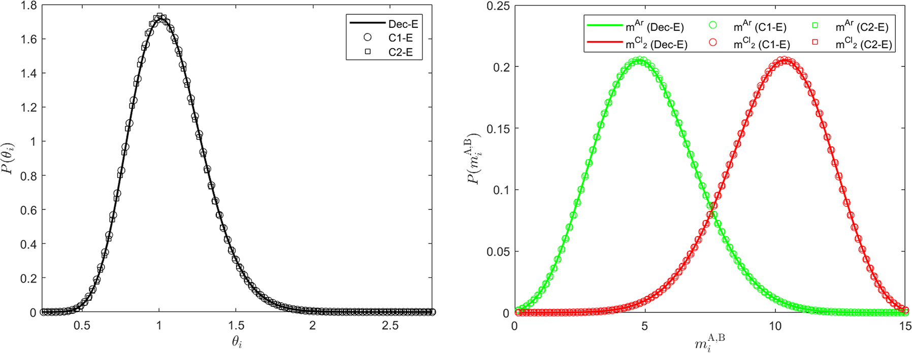
The equilibrium probability distributions of the particle temperature (top) and embedded species masses (bottom) for the CG equimolar Ar/Cl2 binary mixture at an initial temperature T = 1.081 and system number density c = 0.3152, as obtained from the decoupled GenDPDE-M simulation, Dec-E, and coupled GenDPDE-M simulations C1-E and C2-E. All the distributions consistently overlap.
From Figure 1, we can see that P(θ
i
) as well as
4.2 Non-equilibrium simulations
Non-equilibrium simulations of the CG equimolar Ar/Cl2 binary mixture were carried out for an initial state T = 0.885 and c = 0.5775, corresponding again to supercritical conditions for the pure substances. Six GenDPDE-M tests were performed, in which we set γ = 4.5, κ = 1 and Ð = 5, and varied L um according to the values of k u and k m given in Table 2. Notice that the mesoscopic Maxwell–Stefan coefficient Ð was increased with respect to the equilibrium simulations to allow the system to quickly relax to steady-state conditions, thus reducing the computational cost of the tests. A short equilibration run of n equil = 1 × 10⁵ timesteps was performed before imposing heat transfer between the hot and cold slabs. A relaxation period of n relax = 4 × 10⁵ timesteps was subsequently considered, after which no variation in the average temperature and concentration profiles was observed.
Parameters employed in non-equilibrium GenDPDE-M simulations. The coupling constants k u and k m are energy and mass prefactors with the dimensions of k B . L um is the mesoscopic Onsager’s cross-coefficient defined in Eq. (72). n run is the selected number of simulation timesteps.
| Test | k u | k m | L um | n run |
|---|---|---|---|---|
| Dec-NE | 2.0000 | 2.0000 | 0.0 | 1.5 × 10⁶ |
| C1-NE | 1.5000 | 0.6072 | −1.0 | 1.5 × 10⁶ |
| C2-NE | 1.8000 | 0.4830 | −1.5 | 1.5 × 10⁶ |
| C3-NE | 0.5000 | 1.3929 | 1.0 | 1.5 × 10⁶ |
| C1b-NE | 0.9000 | 0.1440 | −1.0 | 1.5 × 10⁶ |
| C2b-NE | 1.1000 | 0.0200 | −1.5 | 1.5 × 10⁶ |
Similarly to the equilibrium cases, here test Dec-NE refers to a decoupled system simulating the same algorithm as in Refs. [24], [25]. As shown in Table 2, tests C1-NE, C2-NE and C3-NE consider coupled configurations with different strengths of the dynamic energy-mass coupling effect, controlled by the value of the coefficient L um . Furthermore, with the aim of assessing the independence of the results from the choice of k u and k m provided that L um is kept constant, simulations C1b-NE and C2b-NE were performed, testing identical conditions to the cases C1-NE and C2-NE, respectively, but using different values of the coupling constants.
Figure 2 shows the steady-state profiles of the local average particle dressed temperature, T(x) = ⟨θ(x)⟩, which is a possible estimator of the local temperature. Notice that, if the bare temperature
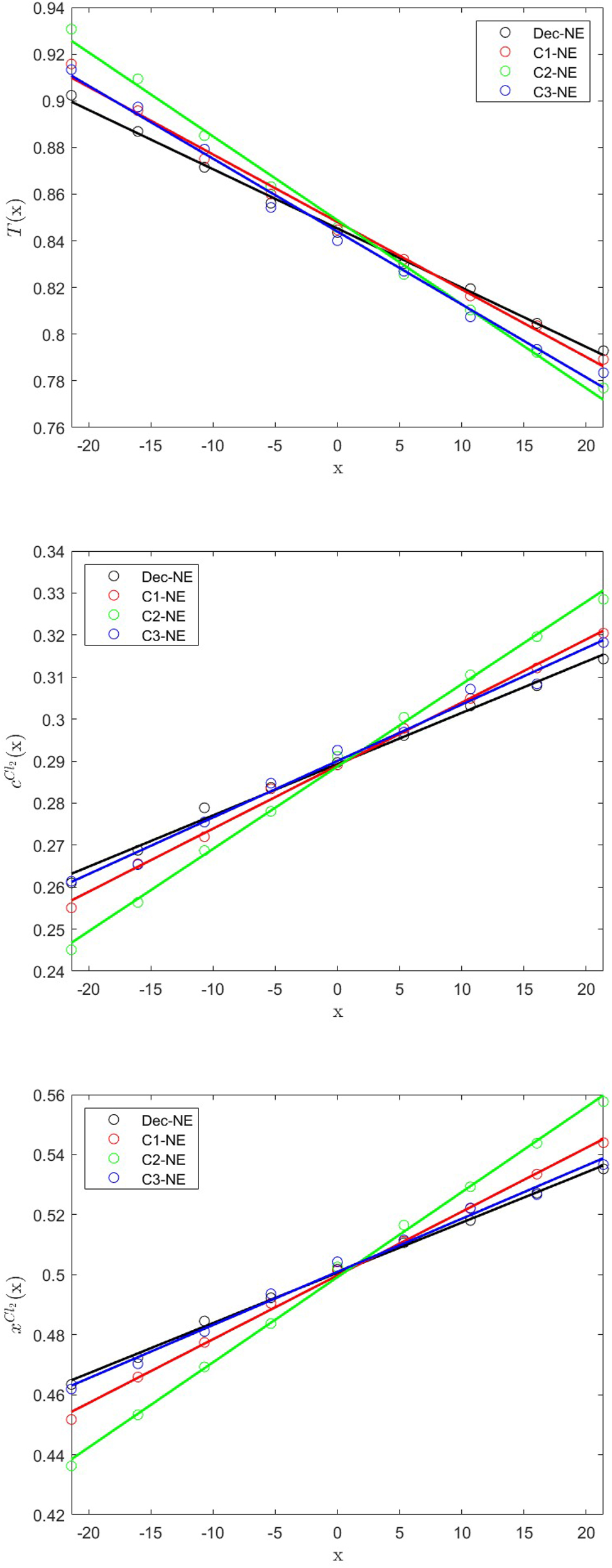
The x-profiles of the particle temperature (top), and the number concentration (middle) and molar fraction (bottom) of Cl2 for the CG equimolar Ar/Cl2 binary mixture at an initial temperature T = 0.885 and system number density c = 0.5775, as obtained from the decoupled GenDPDE-M simulation, Dec-NE, and coupled GenDPDE-M simulations C1-NE, C2-NE and C3-NE. The circles represent simulation results, while the solid lines represent linear regressions.
In Figure 3 we analyze the results of the aforementioned pairs of analogous cases, namely C1-NE and C1b-NE, as well as C2-NE and C2b-NE. The temperature, concentration and molar fraction profiles observed for cases C1b-NE and C2b-NE are practically indiscernable when compared to tests C1-NE and C2-NE, respectively: this result proves that the overall macroscopic behavior of our model is indeed insensitive to the specific values of the coupling constants k u and k m , and depends only on the parameters κ and Ð and on the coupling coefficient L um .
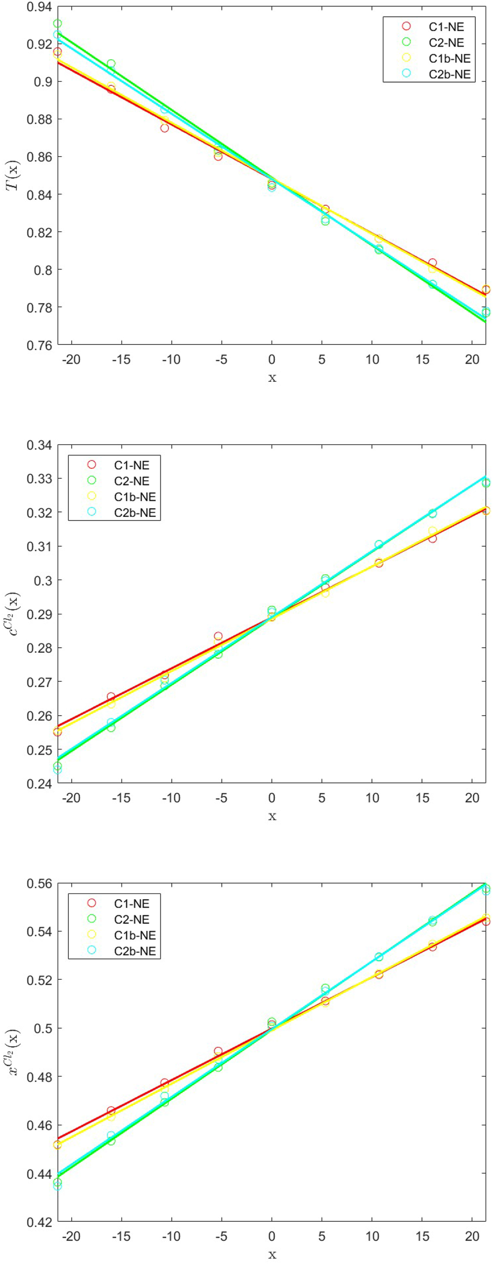
The x-profiles of the particle temperature (top), and the number concentration (middle) and molar fraction (bottom) of Cl2 for the CG equimolar Ar/Cl2 binary mixture at an initial temperature T = 0.885 and system number density c = 0.577, as obtained from the coupled GenDPDE-M simulations C1-NE and C2-NE and their analogous C1b-NE and C2b-NE. The circles represent simulation results, while the solid lines represent linear regressions. The results referring to identical sets of mesoscopic dynamic coefficients are in excellent agreement.
From the profiles T(x) and x
B(x), we evaluated the corresponding gradients, dT/dx and dx
B/dx, using linear regressions, and computed the thermal conductivity, λ, as well as the Soret coefficient,
Values of the thermal conductivity, λ, and the Soret coefficient for Cl2,
| Test | J x × 103 | (dT/dx) × 103 |
|
λ |
|
|---|---|---|---|---|---|
| Dec-NE | 6.46 | −2.54 ± 0.05 | 1.67 ± 0.03 | 2.55 ± 0.05 | 2.64 ± 0.07 |
| C1-NE | 6.46 | −2.89 ± 0.09 | 2.12 ± 0.04 | 2.23 ± 0.07 | 2.94 ± 0.10 |
| C2-NE | 6.46 | −3.60 ± 0.10 | 2.84 ± 0.05 | 1.80 ± 0.05 | 3.15 ± 0.10 |
| C3-NE | 6.46 | −3.12 ± 0.10 | 1.77 ± 0.06 | 2.07 ± 0.07 | 2.27 ± 0.11 |
| C1b-NE | 6.46 | −2.95 ± 0.06 | 2.21 ± 0.02 | 2.19 ± 0.05 | 2.99 ± 0.07 |
| C2b-NE | 6.46 | −3.47 ± 0.07 | 2.80 ± 0.06 | 1.86 ± 0.04 | 3.22 ± 0.10 |
We observe that the measured errors in the determination of both λ and
4.3 Scale-dependence of the mesoscopic model
To conclude this section, we briefly consider the analysis of the system properties as a function of the degree of CGing, Φ. Although this issue will be examined more thoroughly elsewhere, let us introduce here a minimal model, satisfying the GenDPDE-M dynamics discussed in this manuscript, in which the scale factor Φ = 1 and its number of mesoparticles N
0 is of the order of the total number of physical particles in the system,
where ζ(Φ) is proportional to the integration of the product of the weight function w with the pair distribution function g over the cutoff radius R cut, ζ = ∫dr w(r)g(r). This parameter measures the local inhomogeneities in the particle distribution due to the presence of the interparticle pair potential interaction at the present degree of CGing. Hence, from Eq. (83), we can write Eq. (100) as
In addition, we consider that
To numerically illustrate these facts, we have conducted simulations at different degrees of CGing. Figure 4 shows the variation of the system pressure P and the internal energy per particle u = U/N
0 as a function of Φ for an equimolar Ar/Cl2 mixture at a temperature T = 0.885 and number density c = 0.5775, as obtained from GenDPDE-M simulations. The figure also illustrates the effect of the number of neighbors, which depends on the chosen value of the cutoff radius. In our analysis, two different nominal cutoff radii were used, namely,

The system internal energy per physical particle (top) and the system pressure (bottom) as functions of the level of CGing, for an equimolar Ar/Cl2 mixture at an initial temperature T = 0.885 and system number density c = 0.5775. The thermodynamic u = 0.56, and the thermodynamic P = 1.44.
5 Conclusions
The Generalized Energy-Conserving Dissipative Particle Dynamics with Mass Transfer method (GenDPDE-M) was introduced in Refs. [24], [25] as an extension of the GenDPDE algorithm to simulate mesoparticles with variable composition. These original publications, being a proof of concept, only dealt with the particular case in which energy and mass transport between particles were dynamically decoupled. In real systems, however, it is well known that the energy fluxes entrain mass transport, and vice versa, leading to the Ludwig–Soret and Dufour effects [26]. In this article, we have developed the theoretical framework required to describe such coupled energy and material transport at the mesoscale. With this addition, GenDPDE-M can simulate general complex physicochemical scenarios in which the simultaneous transport of energy and matter takes place at the mesoscale; the method is therefore complete.
The extension presented in this article is formulated through the introduction of novel forms for the heat and diffusive fluxes between the mesoparticles. Here, these fluxes depend on both temperature and chemical potential differences, following Onsager’s formulation of non-equilibrium thermodynamics. Since the GenDPDE-M method is formulated as Langevin-like equations, with random contributions simulating the effect of the hydrodynamic fluctuations [3], expressions for the amplitudes of these random terms need to be derived. Starting from Detailed Balance as the physical link between the mesoscopic model and the underlying physical system, we obtained the necessary Fluctuation-Dissipation theorems providing these amplitudes as functions of particle state variables, such as temperature, and also on the dynamic coefficients, which include the coupling. Interestingly, Detailed Balance is sufficient to also demonstrate that Onsager’s reciprocal relations are valid at the mesoscale.
The consistency of the algorithm is demonstrated by showing that the simulated dynamics effectively samples the equilibrium probability distributions indicated in Eq. (67). We have checked that the distributions are independent of the values of the mesoscopic transport coefficients as well as the dynamic coupling between energy and mass. For completeness, a non-equilibrium simulation scheme, analogous to the setup of a real experiment, was conceived with the aim of reproducing the Ludwig–Soret effect for a specific two-component system. The mesoscopic thermodynamic model employed was the van der Waals one-fluid model describing an Ar/Cl2 mixture. It is shown that GenDPDE-M not only properly reproduces this phenomenon, but crucially also allows us to control the strength of the Ludwig–Soret effect through the appropriate choice of the mesoscopic Onsager’s cross-coefficient
The framework developed in this article aims at the simulation of multicomponent systems, including moving interfaces, which are particularly relevant in areas such as chemical engineering, heat transport, materials engineering, among many others. The most natural step forward is to extend the algorithm to include chemical reactions within the mesoparticles, coupled to energy and matter transport, which will permit the simulation of reactive systems with moving interfaces, e.g., detonation and combustion, interfacial growth, among many other situations in which complex fluid processes may take place. Such an extension will be done elsewhere. Furthermore, the use of more complex EoS for the particle thermodynamic description, such as the Lennard–Jones [31], [39], Exponential-6 [40], [41], [42] or Statistical Associated Fluid Theory [43] EoS, enables the application of the method to a panoply of different materials and processes.
-
Research ethics: Not applicable.
-
Author contributions: The authors have accepted responsibility for the entire content of this manuscript and approved its submission.
-
Competing interests: The authors state no conflict of interest.
-
Research funding: GC acknowledges funding from the European Union’s Horizon 2020 research and innovation programme under the Marie Skłodowska-Curie grant agreement No. 945413 (DOI 10.3030/945413) and from the Universitat Rovira i Virgili (URV). AM and JBA acknowledge support from the grant PID2021-122187NB-C33, funded by MCIN/AEI/10.13039/501100011033 and “ERDF A way of making Europe”. Research performed by AM and JBA was furthermore sponsored by the Army Research Office (DOI 10.13039/100000183), and was accomplished under Cooperative Agreement No. W911NF-20-2-0227. Research performed by ML was sponsored by the Army Research Office and was accomplished under Cooperative Agreement No. W911NF-20-2-0203. ML also acknowledges funding from the Czech Science Foundation (DOI 10.13039/501100001824), grant No. 21-27338S. JPL and JKB acknowledge support in part for a grant of computer time from the DoD High Performance Computing Modernization Program at the Army, Navy, and Air Force Supercomputing Resource Centers.
-
Data availability: The raw data can be obtained on request from the corresponding author.
-
Disclaimer: This work reflects only the author's view and the Agency is not responsible for any use that may be made of the information it contains. The views and conclusions contained in this document are those of the authors and should not be interpreted as representing the official policies, either expressed or implied, of the Army Research Office or the U.S. Government. The U.S. Government is authorized to reproduce and distribute reprints for Government purposes notwithstanding any copyright notation herein.
Appendix A: Alternative formulation of the heat and diffusive fluxes
With the purpose of exploring the possible definition of alternative expressions for the heat and diffusive fluxes, defined in Eqs. (34) and (35), let us introduce the following definitions:
In view of these equations, the condition
After some algebra, Eq. (A5) becomes
We recall that the bare chemical potential is a function of the bare temperature, according to Eqs. (94) and (95). Hence, the quantities
where
According to our formulation of the particle dynamics, the mass and energy transfer occur at constant local density, as the kinematic move takes place separately from thermodynamic property exchange moves. Hence, we must consider that the transfer occurs at constant volume (or local density n). Therefore, rather than proceeding by introducing ∂μ/∂θ| π = −s, as is usually done, we have instead ∂μ/∂θ| n = −s − (n/κ T )∂μ/∂π| θ , as the processes are not at constant pressure.
At this point, it is rather obvious that the analogy with the macroscopic definition of the measurable heat flux cannot be continued further. From one perspective, the expansion of the thermodynamic properties around the central temperature precludes the possibility of having large particle temperature differences, which may be present in some situations of interest for the application of our model. Notice that, even in equilibrium, the temperature differences between particles are of the order of
cannot be related to the particle entropies, as
where again we have retained terms up to the first order only. Further, manipulating Eq. (A10) by introducing
we can write,
where we have defined what would be the analogous expression of the measurable heat flux at the mesoscale, i.e.,
Although we show that, under specific thermodynamic conditions the measurable heat flux can be defined, we stress that the quantity
Appendix B: Fluctuation-Dissipation theorem
The relation between the matrices containing the mesoscopic transport coefficients, L ij , and the amplitudes of the random terms, σ ij , as defined in Eq. (48) follows from the evaluation of the second moment of the system distribution [11], [12] and use of DB. We remind the reader that the validity of DB is only based on the form of the Hamiltonian of the underlying microscopic physical system, together with the time-reversibility of the trajectories of the latter [44]. Therefore, as GenDPDE-M aims at simulating physical systems, the assumption of DB is the most basic assumption that connects its structure to the physical nature of the processes of the system.
Thus, the second moment of the fluctuating mesoscopic state vector x i , defined in Eq. (47) is given by
where
due to causality. Here,
Here, we have only considered a given pair of mesoparticles i and j as the FD theorem has to be satisfied by any given number of pairs, which ultimately implies it should be satisfied individually for every pair. In view of this, we have restricted our demonstration to a given pair for simplicity of notation and clarity, but with no loss of generality. Hence,
Note that the first term on the right-hand side of Eq. (B3) is exactly
Next, let us focus on individual terms on the right-hand side of Eq. (B4) separately. We start with rewriting the second term as
where partial integration and independence of L
ij
from u
i
and
Finally, the third term can be rewritten as
where use has been made of the properties of the normalized random numbers, Eqs. (43) and (44), together with Eq. (47). Inserting Eqs. (B5)–(B7) into (B4), we get
As we demand that the dynamic coefficients of the model be independent of the reservoir characteristics contained in
Equation (B9) represents the general FD theorem relating the mesoscopic transport coefficients to the amplitudes of the thermal fluctuations.
Appendix C: Onsager’s reciprocal relations
Demonstration of Onsager’s reciprocal relations for the mesoscopic transport coefficients follows from the evaluation of the autocorrelation of the state vectors at different times, i.e.,
Using the compact form of the EoM Eq. (46), together with the property of the transition probability Eq. (B2) and the fact that the random terms are not correlated to other state variables at the same instant of time, we can rewrite Eq. (C1) as
Analogously to Appendix B, in this demonstration we only consider a pair of mesoparticles, namely i and j, as the validity of ORR should be independent of the number of pairs. Next, using DB [44],
it follows that
where
Equating the right-hand sides of Eqs. (C2) and (C3), and using the properties of the transposed matrix, we get
The above integrals were already solved in Eqs. (B5) and (B6). Invoking again the independence of L ij from the reservoir properties, Eq. (C4) is satisfied if we further demand that
Therefore, we conclude that, for a binary mixture, the condition
References
[1] P. J. Hoogerbrugge and J. M. V. A. Koelman, “Simulating microscopic hydrodynamic phenomena with dissipative particle dynamics,” Europhys. Lett., vol. 19, no. 3, pp. 155–160, 1992. https://doi.org/10.1209/0295-5075/19/3/001.Search in Google Scholar
[2] J.-P. Hansen and I. R. McDonald, Theory of Simple Liquids, Oxford, Elsevier, 2006.Search in Google Scholar
[3] L. D. Landau and E. M. Lifshitz, Fluid Mechanics. Landau and Lifshitz: Course of Theoretical Physics, vol. 6, 2nd ed Oxford, Pergamon, 1987.Search in Google Scholar
[4] P. Español and P. B. Warren, “Statistical mechanics of dissipative particle dynamics,” Europhys. Lett., vol. 30, no. 4, pp. 191–196, 1995. https://doi.org/10.1209/0295-5075/30/4/001.Search in Google Scholar
[5] J. B. Avalos and A. D. Mackie, “Dissipative particle dynamics with energy conservation,” Europhys. Lett., vol. 40, no. 2, pp. 141–146, 1997. https://doi.org/10.1209/epl/i1997-00436-6.Search in Google Scholar
[6] P. Español, “Dissipative particle dynamics with energy conservation,” Europhys. Lett., vol. 40, no. 6, pp. 631–636, 1997. https://doi.org/10.1209/epl/i1997-00515-8.Search in Google Scholar
[7] R. Qiao and P. He, “Simulation of heat conduction in nanocomposite using energy-conserving dissipative particle dynamics,” Mol. Simul., vol. 33, no. 8, pp. 677–683, 2007. https://doi.org/10.1080/08927020701286511.Search in Google Scholar
[8] G. C. Ganzenmüller, S. Hiermaier, and M. O. Steinhauser, “Shock-wave induced damage in lipid bilayers: a dissipative particle dynamics simulation study,” Soft Matter, vol. 7, no. 9, pp. 4307–4317, 2011. https://doi.org/10.1039/c0sm01296c.Search in Google Scholar
[9] Z. Li, Y.-H. Tang, X. Li, and G. E. Karniadakis, “Mesoscale modeling of phase transition dynamics of thermoresponsive polymers,” Chem. Commun., vol. 51, no. 55, pp. 11038–11040, 2015. https://doi.org/10.1039/c5cc01684c.Search in Google Scholar PubMed
[10] E. O. Johansson, T. Yamada, B. Sundén, and J. Yuan, “Modeling mesoscopic solidification using dissipative particle dynamics,” Int. J. Therm. Sci., vol. 101, pp. 207–216, 2016, https://doi.org/10.1016/j.ijthermalsci.2015.11.002.Search in Google Scholar
[11] J. Bonet Avalos, M. Lísal, J. P. Larentzos, A. D. Mackie, and J. K. Brennan, “Generalised dissipative particle dynamics with energy conservation: density- and temperature-dependent potentials,” Phys. Chem. Chem. Phys., vol. 21, no. 45, pp. 24891–24911, 2019. https://doi.org/10.1039/c9cp04404c.Search in Google Scholar PubMed
[12] J. Bonet Avalos, M. Lísal, J. P. Larentzos, A. D. Mackie, and J. K. Brennan, “Generalised dissipative particle dynamics with energy conservation revisited: insight from the thermodynamics of the mesoparticle leading to an alternative heat flow model,” Phys. Rev. E, vol. 103, no. 6, p. 062128, 2021. https://doi.org/10.1103/physreve.103.062128.Search in Google Scholar
[13] I. Pagonabarraga and D. Frenkel, “Dissipative particle dynamics for interacting systems,” J. Chem. Phys., vol. 115, no. 11, pp. 5015–5026, 2001. https://doi.org/10.1063/1.1396848.Search in Google Scholar
[14] P. B. Warren, “Vapor-liquid coexistence in many-body dissipative particle dynamics,” Phys. Rev. E, vol. 68, no. 6, p. 066702, 2003. https://doi.org/10.1103/physreve.68.066702.Search in Google Scholar
[15] E. Moeendarbary, T. Y. Ng, and M. Zangeneh, “Dissipative particle dynamics: introduction, methodology and complex fluid applications – a review,” Int. J. Appl. Mech., vol. 1, no. 4, pp. 737–763, 2009. https://doi.org/10.1142/s1758825109000381.Search in Google Scholar
[16] J. K. Brennan, M. Lísal, J. D. Moore, S. Izvekov, I. V. Schweigert, and J. P. Larentzos, “Coarse-grain model simulations of nonequilibrium dynamics in heterogeneous materials,” J. Phys. Chem. Lett., vol. 5, no. 12, pp. 2144–2149, 2014. https://doi.org/10.1021/jz500756s.Search in Google Scholar PubMed
[17] J. D. Moore, et al., “A coarse-grain force field for RDX: density dependent and energy conserving,” J. Chem. Phys., vol. 144, no. 10, p. 104501, 2016. https://doi.org/10.1063/1.4942520.Search in Google Scholar PubMed
[18] P. Español and P. B. Warren, “Perspective: dissipative particle dynamics,” J. Chem. Phys., vol. 146, no. 15, p. 150901, 2017. https://doi.org/10.1063/1.4979514.Search in Google Scholar PubMed
[19] J. P. Larentzos, J. M. Mansell, M. Lísal, and J. K. Brennan, “Coarse-grain modelling using an equation-of-state many-body potential: application to fluid mixtures at high temperature and high pressure,” Mol. Phys., vol. 116, no. 21–22, pp. 3271–3282, 2018. https://doi.org/10.1080/00268976.2018.1459920.Search in Google Scholar
[20] K. P. Santo and A. V. Neimark, “Dissipative particle dynamics simulations in colloid and interface science: a review,” Adv. Colloid Interface Sci., vol. 298, p. 102545, 2021, https://doi.org/10.1016/j.cis.2021.102545.Search in Google Scholar PubMed
[21] Z. Li, Y.-H. Tang, H. Lei, B. Caswell, and G. E. Karniadakis, “Energy-conserving dissipative particle dynamics with temperature-dependent properties,” J. Comput. Phys., vol. 265, pp. 113–127, 2014, https://doi.org/10.1016/j.jcp.2014.02.003.Search in Google Scholar
[22] M. Lísal, J. P. Larentzos, J. B. Avalos, A. D. Mackie, and J. K. Brennan, “Generalized energy-conserving dissipative particle dynamics with reactions,” J. Chem. Theory Comput., vol. 18, no. 4, pp. 2503–2512, 2022. https://doi.org/10.1021/acs.jctc.1c01294.Search in Google Scholar PubMed
[23] B. H. Lee, M. N. Sakano, J. P. Larentzos, J. K. Brennan, and A. Strachan, “A coarse-grain reactive model of RDX: molecular resolution at the μm scale,” J. Chem. Phys., vol. 158, no. 2, p. 024702, 2023. https://doi.org/10.1063/5.0122940.Search in Google Scholar PubMed
[24] J. B. Avalos, M. Lísal, J. P. Larentzos, A. D. Mackie, and J. K. Brennan, “Generalized energy-conserving dissipative particle dynamics with mass transfer. Part 1: theoretical foundation and algorithm,” J. Chem. Theory Comput., vol. 18, no. 12, pp. 7639–7652, 2022. https://doi.org/10.1021/acs.jctc.2c00452.Search in Google Scholar PubMed
[25] M. Lísal, J. B. Avalos, J. P. Larentzos, A. D. Mackie, and J. K. Brennan, “Generalized energy-conserving dissipative particle dynamics with mass transfer. Part 2: applications and demonstrations,” J. Chem. Theory Comput., vol. 18, no. 12, pp. 7653–7670, 2022. https://doi.org/10.1021/acs.jctc.2c00453.Search in Google Scholar PubMed
[26] S. R. de Groot and P. Mazur, Non-Equilibrium Thermodynamics, New York, Dover Publications, INC., 1984.Search in Google Scholar
[27] R. Taylor and R. Krishna, Multicomponent Mass Transfer, New York, Wiley, 1993.Search in Google Scholar
[28] L. Onsager and S. Machlup, “Fluctuations and irreversible processes,” Phys. Rev., vol. 91, no. 6, pp. 1505–1512, 1953. https://doi.org/10.1103/physrev.91.1505.Search in Google Scholar
[29] H. B. Callen, Thermodynamics and an Introduction to Thermostatistics, New York, John Wiley & Sons, 1985.Search in Google Scholar
[30] J. Armstrong and F. Bresme, “Thermal conductivity of highly asymmetric binary mixtures: how important are heat/mass coupling effects?,” Phys. Chem. Chem. Phys., vol. 16, no. 24, pp. 12307–12316, 2014. https://doi.org/10.1039/c4cp00818a.Search in Google Scholar PubMed
[31] J. K. Johnson, J. A. Zollweg, and K. E. Gubbins, “The Lennard-Jones equation of state revisited,” Mol. Phys., vol. 78, no. 3, pp. 591–618, 1993. https://doi.org/10.1080/00268979300100411.Search in Google Scholar
[32] J. R. Elliott and T. C. Lira, Introductory Chemical Engineering Thermodynamics, New York, Prentice Hall, 2012.Search in Google Scholar
[33] T. Y. Kwak and G. A. Mansoori, “Van der Waals mixing rules for cubic equations of state. applications for supercritical fluid extraction modelling,” Chem. Eng. Sci., vol. 41, no. 5, pp. 1303–1309, 1986. https://doi.org/10.1016/0009-2509(86)87103-2.Search in Google Scholar
[34] M. Lísal, J. K. Brennan, and J. B. Avalos, “Dissipative particle dynamics at isothermal, isobaric, isoenergetic, and isoenthalpic conditions using Shardlow-like splitting algorithms,” J. Chem. Phys., vol. 135, no. 20, p. 204105, 2011. https://doi.org/10.1063/1.3660209.Search in Google Scholar PubMed
[35] J. P. Larentzos, J. K. Brennan, J. D. Moore, M. Lísal, and W. D. Mattson, “Parallel implementation of isothermal and isoenergetic dissipative particle dynamics using Shardlow-like splitting algorithms,” Comput. Phys. Commun., vol. 185, no. 7, pp. 1987–1998, 2014. https://doi.org/10.1016/j.cpc.2014.03.029.Search in Google Scholar
[36] L. B. Lucy, “A numerical approach to the testing of the fission hypothesis,” Astron. J., vol. 82, pp. 1013–1024, 1977, https://doi.org/10.1086/112164.Search in Google Scholar
[37] F. Müller-Plathe and P. Bordat, “Reverse non-equilibrium molecular dynamics,” Lect. Notes Phys., vol. 640, pp. 310–326, 2004, https://doi.org/10.1007/978-3-540-39895-0_10.Search in Google Scholar
[38] C. Nieto-Draghi and J. B. Avalos, “Non-equilibrium momentum exchange algorithm for molecular dynamics simulation of heat flow in multicomponent systems,” Mol. Phys., vol. 101, no. 14, pp. 2303–2307, 2003. https://doi.org/10.1080/0026897031000154338.Search in Google Scholar
[39] J. Kolafa and I. Nezbeda, “The Lennard-Jones fluid: an accurate analytic and theoretically-based equation of state,” Fluid Phase Equil., vol. 100, pp. 1–34, 1994, https://doi.org/10.1016/0378-3812(94)80001-4.Search in Google Scholar
[40] H. Vörtler, I. Nezbeda, and M. Lísal, “The exp-6 potential fluid at very high pressures: computer simulations and theory,” Mol. Phys., vol. 92, no. 5, pp. 813–824, 1997. https://doi.org/10.1080/00268979709482153.Search in Google Scholar
[41] M. Lísal, W. R. Smith, and I. Nezbeda, “Computer simulation of the thermodynamic properties of high-temperature chemically-reacting plasmas,” J. Chem. Phys., vol. 113, no. 12, pp. 4885–4895, 2000. https://doi.org/10.1063/1.1289245.Search in Google Scholar
[42] J.-X. Sun, Q. Wu, L. Cai, and F. Jing, “Analytic equation of state for exponential-six fluid based on the ross variational perturbation theory and the Percus–Yevick radial distribution function of hard spheres,” Chem. Phys. Lett., vol. 449, no. 1, pp. 72–76, 2007. https://doi.org/10.1016/j.cplett.2007.10.019.Search in Google Scholar
[43] W. G. Chapman, K. E. Gubbins, G. Jackson, and M. Radosz, “New reference equation of state for associating liquids,” Ind. Eng. Chem. Res., vol. 29, no. 8, pp. 1709–1721, 1990. https://doi.org/10.1021/ie00104a021.Search in Google Scholar
[44] N. G. van Kampen, Stochastic Processes in Physics and Chemistry, Amsterdam, North Holland, 1992.Search in Google Scholar
© 2024 the author(s), published by De Gruyter, Berlin/Boston
This work is licensed under the Creative Commons Attribution 4.0 International License.
Articles in the same Issue
- Frontmatter
- Original Research Articles
- Optimization analysis of an endoreversible quantum heat engine with efficient power function
- Heat transfer within nonequilibrium dense aluminum heated by a heavy ion beam
- Thermal and electrical properties of photovoltaic cell with linear phenomenological heat transfer law
- Modeling equilibrium and non-equilibrium thermophysical properties of liquid lubricants using semi-empirical approaches and neural network
- Proposing a procedure for multi-objective optimization of cascade thermoelectric coolers to achieve maximum cooling capacity and COP
- Inconsistency between the micropolar theory and non-equilibrium thermodynamics in the case of polar fluids
- Generalized energy-conserving dissipative particle dynamics with mass transfer: coupling between energy and mass exchange
- Power and efficient power optimization of one-qubit Novikov quantum heat engines with an external dissipative heat leak
- Application of discrete symmetry to natural convection in vertical porous microchannels
- Erratum
- Corrigendum to: Significance of entropy generation and the Coriolis force on the three-dimensional non-Darcy flow of ethylene-glycol conveying carbon nanotubes (SWCNTs and MWCNTs)