The mF mode of authenticated encryption with associated data
-
Bishwajit Chakraborty
 and
Mridul Nandi
and
Mridul Nandi

Abstract
In recent years, the demand for lightweight cryptographic protocols has grown immensely. To fulfill this necessity, the National Institute of Standards and Technology (NIST) has initiated a standardization process for lightweight cryptographic encryption. NIST’s call for proposal demands that the scheme should have one primary member that has a key length of 128 bits, and it should be secure up to
1 Introduction
Lighweight cryptography. Lightweight cryptography is concerned with a huge variety of resource-limited devices including Internet of Things end nodes and radio-frequency identification tags [1]. For a resource-constrained environment, the standard cryptographic protocols such as Advanced Encryption Standard (AES) [2] and SHA3 [3], which work well together, within computer systems, are difficult to implement because of implementation size, speed or throughput, and energy consumption. The lightweight cryptography trades off implementation cost, speed, security, performance, and energy consumption on resource-limited devices. The purpose of lightweight cryptography is to consume less memory, less computing resource, and less power supply, and to provide a weaker but satisfactory security solution that can work in resource-limited devices. As a consequence, lightweight cryptographic protocols are expected to be simpler and faster as compared to conventional cryptographic protocols.
In the last decade, the demand for lightweight cryptographic protocols has grown immensely. To fulfill this necessity, the National Institute of Standards and Technology (NIST) has initiated a standardization process for lightweight cryptographic (LWC) encryption schemes. NIST’s call for proposal [4] demands that a scheme should have one primary member that has a key length of 128 bits, and it should be secure up to
(Tweakable) block cipher. A block cipher is a cryptographic primitive consisting of two algorithms, namely,
A tweakable block cipher (TBC) [5] is a deterministic function
TBC-based AEAD. For many AEAD modes [6,7,8, 9,10] with an underlying TBC
where
Security of some instantiations of TBC based on block ciphers. A dedicated TBC construction is conjectured to have security, and hence, we can instantiate the mode by such a secure TBC. In addition to the dedicated constructions, there are some known constructions of TBC based on a block cipher. For example, XEX [11] is shown to have birthday-bound security.
AEAD modes such as
Note that while constructing any TBC, it is generally desired that it should achieve security with a
Can we have an instantiation of TBC based on block cipher without using any auxiliary key but still provide satisfactory security (for instance, up to the NIST desired level)?
At a glance, it seems impossible to design such a TBC. However, we show that such security is possible to achieve for the AEAD mode based on a TBC, which does not use any auxiliary key. Clearly, we must have different reductions than what we usually have (as mentioned in equations (1.1)–(1.2)). The distinguishing attack for
1.1 Our contribution
We formalize the TBC-based AEAD mode, which is used in
where the new security advantage terms
We now study these two security notions for two instantiations of TBC.
Plugging these results in our previous results, we obtain that the
1.2 Organization of the article
In Section 2, we define some existing and newly introduced security definitions associated with AEAD modes and TBCs. In Section 3, we introduce the TBC-based AEAD scheme called
2 Security definitions of AEAD and TBC
2.1 Security definitions of AEAD
In this section, we define some well-known security definitions of AEAD modes. We call an AEAD adversary nonce respecting when it doesn’t make more than one encryption query with the same nonce. An authenticated encryption scheme with associated data functionality, or AEAD in short, is a tuple of deterministic algorithms
Here,
2.1.1 Privacy
Given an adversary
where the maximum is taken over all the nonce-respecting adversaries
2.1.2 Forgery
We say that a nonce-respecting oracle adversary
and we write
where the maximum is taken over all adversary
2.2 Security definitions of TBC
Let
where
Next, we define two new security definitions for a given TBC.
2.2.1
μ
-respecting TPRP security
Let
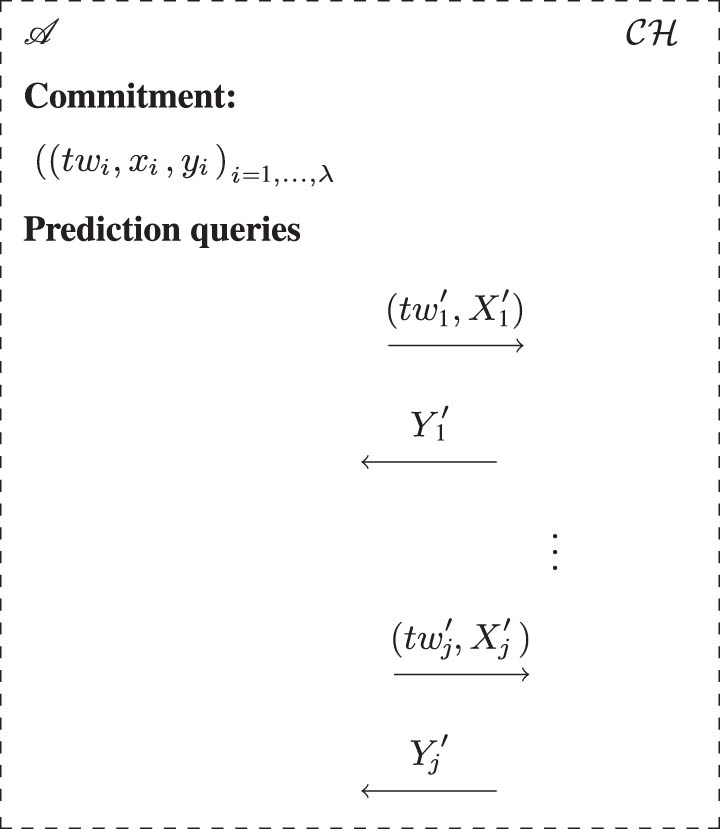
2.2.2 Multi-commitment prediction
Let
PHASE 2:
After all the queries of the first phase are done, it makes at most
We say that any adversary
The
and we write,
where maximum is taken over all adversaries
We define
where the maximum is taken over all adversaries as defined earlier with the additional restriction that they make
We would like to note that in the ideal cipher model, the
2.3 Multi collision
We say that an adversary
and
Phase 2 of the
3 The
mF
mode of AEAD
We start by defining the positive feedback function
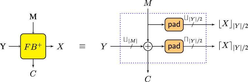
The
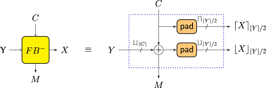
The FB − function in mF. pad is 0 1 ∗ padding.
Let
Given any data
Associated data processing: It parses
Message processing: It parses
Let
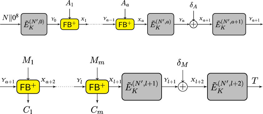
Block diagram for mF encryption. Here, N′ = N‖x, where x = 08/07 1 depending on the condition that (a ≠ 0) or (a = 0 & m ≠ 0) respectively. We define l = a + m. δ A , δ M are as defined in Figure 5.
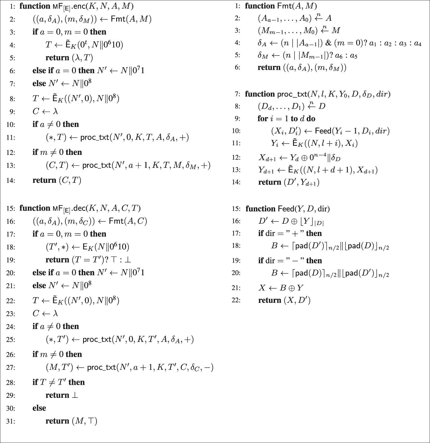
Algorithm defining the
4 Security reductions of
mF
Here, we give upper bounds on the privacy advantage and forging advantage of
4.1 Privacy
Theorem 4.1
For any privacy adversary
where
Proof
Note that
By using straightforward reduction, one can construct an adversary
The inequality (1) follows from the definition that
Consider the event that
for some known
Then, clearly,
Finally, to bound
The
Note that the probability of
In that case, for a given
Varying over all
Hence, we have
Lemma 4.2
4.2 Forgery
Define an oracle
We can similarly define
This follows from the standard reduction and Lemma 4.2.
Theorem 4.3
For any nonce-respecting forging adversary
Let
4.2.1 The reduction game
Let
Phase 1:
Whenever
In the previous step,
For every decryption query of the form
When all the encryption and decryption queries by
if there doesn’t exist any encryption query
Else if
Else if
Else if
Else if
If
Remark 4.4
If there exists a common prefix between
Phase 2 (commitment):
For each
If
Note that
If
If
where
Phase 2 (prediction):
For each
If
It calculates
It sends prediction query of the form
If
Note that
Finally
If
Note that,
for
It sends
4.2.2 Understanding the reduction game
The adversary
For simplicity, we assume that
Here, we only discuss the most complex case, i.e., when there exists an encryption query of the form
Note that adversary
Remark 4.5
When
Let CBAD denote the event that
Lemma 4.6
Proof
Since
where
Now, Let
Now since all the
Corollary 4.7
If the event
Proof
Note that,
Proposition 4.8
Suppose
We postpone the proof of Proposition 4.8 to Section 4.3.
4.2.3 Proof of Theorem 4.3
For all encryption queries of the form
Note that Proposition 4.8 means, that, given
Hence,
4.3 Proof of Proposition 4.8
Let
Case 1: If
In the commitment phase, the adversary
Notice that if
If
If
Let
Hence, if any of the aforementioned condition is satisfied, then
Case 2: If
We have,
where
In the commitment phase, the adversary
Case 3: If
There exist an
Now consider the two cases:
First, let
Now, let
Hence, we conclude that
In the commitment phase, the adversary commits
If
If not, then
Hence, we have
Inductively, suppose
Hence,
Since
Finally, since
Hence,
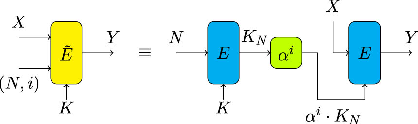
5 A block cipher-based TBC construction
Let
Definition 5.1
Given any fixed KUF
where for all
Notice that if
Consider a block cipher
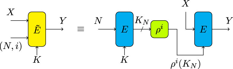
A block cipher-based TBC construction.
Remark 5.2
If the key size
5.1 Bounding
μ
-
TPRP
security of
E
˜
Here, we try to bound the
We assume that the adversary doesn’t make repetitive or redundant queries.
5.1.1 The ideal world and analysis of bad events
Let
In the ideal world, the oracle chooses random functions
Primitive query: In the Ideal world for the ith primitive query of the form
Define
Online query: On receiving the ith input query of the form
Offline computation: Oracle chooses
Define
Define
Bad Events: We now look at the ideal world transcript
Similarly, the six possible output collisions are as follows:
We ignore cases
In notation:
Note that, in the ideal world,
Definition 5.3
We call a transcript
Lemma 5.4
Proof
Here, we try to bound the distinct bad events defined earlier.
Bounding
Bounding
Case 1: (
Case 2: (
Hence, Case 2 event occurs if and only if,
Note that queries of this form arise due to the encryption query of
Let
Now, varying over all possible
Since the aforementioned two cases are mutually exclusive, we have
Bounding
Bounding
Then, by union bound, we have
Bounding
Bounding
Hence, we get
Finally, adding all the probabilities, we get the lemma.□
5.1.2 Real World and good transcript analysis
The real world has oracle
By good transcript, we mean any transcript, which is not bad. Now consider a good transcript
Note that by definition of the good transcript, the input–outputs of
where
Now, note that in the real world, the primitive queries and online queries are permutation compatible.
Hence, we have
Hence,
Hence, by H-coefficient technique, we have Theorem 5.5.
Theorem 5.5
5.2 Bounding
(
μ
,
λ
)
-
m
c
p
security of
E
˜
Here, we try to bound the advantage of a
5.2.1 Game 0:
We define the original
Phase 1:
Primitive query: For the ith primitive query of the form
Define
Online query oracle chooses
Phase 2:
Commitment generation:
Primitive queries:
Prediction queries: Whenever
Let
Define
5.2.2 Game 1:
We now define a newly modified security game called Game 1. Here,
Phase 1 online query: On receiving the ith input query of the form
We say that any adversary
where the maximum is taken over all adversaries
Proposition 5.6
Given any
Proof
We construct the
Whenever
Whenever
On receiving the commitments from
Whenever
Whenever
From the construction, it is clear that whenever
Hence,
□
Proposition 5.7
Proof
Consider the following event due to Phase 2.
Claim 5.8
Proof
Fix
Claim 5.9
Proof
Suppose
Proposition 5.7 follows from Claims 5.8 and 5.9.
Theorem 5.10
Proof
From Proposition 5.6, we have for any
Taking maximum over all such
Now plugging in the appropriate values from Proposition 5.7 and Theorem 4.1, we have Theorem 4.3.□
6
mF
under the new TBC construction
In this section, we consider the
Theorem 6.1
Theorem 6.2
where
Proof
Theorems 6.1 and 6.2 can be derived from Theorems 4.1 and 4.3, respectively, by appropriately plugging in the security bounds for
6.1
mixFeed
as an
mF
construction
The
Khairallah [13] observed that
7 Overcoming the weakness of
mixFeed
In this section, we show that the weakness in
For any primitive polynomial
Next, we consider the
Theorem 7.1
Theorem 7.2
where
7.1 Interpretation of the above bounds
According to NIST requirement,
Remark 7.3
If the linearity of multiplication by a primitive polynomial
8
mF
mode as a lightweight AEAD
In this section, we try to give a theoretical comparison between the
A TBC in
We have tabulated theoretical comparisons of different TBC-based AEAD schemes in Table 1. A more practical, implementation-based comparison is beyond the scope of this article and can be left as a future research problem.
A theoretical comparison of different TBC-based lightweight AEAD schemes. Here the TBC of
| Mode | State size (includes key size) | Block size | Tweak size |
|
Bits processed per primitive call | Inverse free |
|---|---|---|---|---|---|---|
| Romulus-N1 [8] | 512 | 128 | 384 | 1 | 128 | Yes |
| Romulus- M1 [8] | 512 | 128 | 384 | 2 | 64 | Yes |
| SKINNY-AEAD (M1) [16] | 640 | 128 | 384 | 1 | 128 | No |
| QAMELEON [17] | 640 | 128 | 384 | 1 | 128 | No |
| LILLIPUT-I-128 [18] | 576 | 128 | 320 | 1 | 128 | No |
|
|
384 | 128 | NA | 1 | 128 | Yes |
9 Conclusion
In this article, we have considered a TBC-based AEAD scheme
-
Conflict of interest: Authors state no conflict of interest.
References
[1] N. Mouha. The design space of lightweight cryptography. in: NIST Lightweight Cryptography Workshop 2015. 2015. Search in Google Scholar
[2] NIST. Announcing the ADVANCED ENCRYPTION STANDARD (AES), National Institute of Standards and Technology, U.S. Department of Commerce, Fedral Information Processing Standards Publication no FIPS 197. 2001.Search in Google Scholar
[3] M. J. Dworkin. SHA-3 standard: Permutation-based hash and extendable-output functions. 2015. 10.6028/NIST.FIPS.202Search in Google Scholar
[4] NIST. Submission Requirements and Evaluation Criteria for the Lightweight Cryptography Standardization Process. 2018.https://csrc.nist.gov/CSRC/media/Projects/Lightweight-Cryptography/documents/final-lwc-submission-requirements-august2018.pdfSearch in Google Scholar
[5] M. Liskov, R.L. Rivest, D. Wagner. Tweakable block ciphers. In: Annual International Cryptology Conference. Springer; 2002. p. 31–46. 10.1007/3-540-45708-9_3Search in Google Scholar
[6] B. Chakraborty, M. Nandi. mixFeed. Submission to NIST LwC Standardization Process (Round 2). 2019. https://csrc.nist.gov/CSRC/media/Projects/lightweight-cryptography/documents/round-2/spec-doc-rnd2/mixFeed-spec-round2.pdf.Search in Google Scholar
[7] T. Iwata, M. Khairallah, K. Minematsu, T. Peyrin. REMUS. Submission to NIST LwC Standardization Process (Round 1). 2019. https://csrc.nist.gov/CSRC/media/Projects/Lightweight-Cryptography/documents/round-1/spec-doc/Remus-spec.pdf.Search in Google Scholar
[8] T. Iwata, M. Khairallah, K. Minematsu, T. Peyrin. Romulus. Submission to NIST LwC Standardization Process (Round 2). 2019. https://csrc.nist.gov/CSRC/media/Projects/lightweight-cryptography/documents/round-2/spec-doc-rnd2/Romulus-spec-round2.pdf. Search in Google Scholar
[9] T. Iwata, M. Khairallah, K. Minematsu, T. Peyrin, Y. Sasaki, S. MengSim, L. Sun. Thank Goodness It’s Friday (TGIF). Submission to NIST LwC Standardization Process (Round 1). 2019. https://csrc.nist.gov/CSRC/media/Projects/Lightweight-Cryptography/documents/round-1/spec-doc/TGIF-spec.pdf.Search in Google Scholar
[10] S. Gueron, A. Jha, M. Nandi. COMET. Submission to NIST LwC Standardization Process (Round 1). 2019. https://csrc.nist.gov/CSRC/media/Projects/lightweight-cryptography/documents/round-2/spec-doc-rnd2/comet-spec-round2.pdf.Search in Google Scholar
[11] P. Rogaway. Efficient instantiations of tweakable blockciphers and refinements to modes OCB and PMAC. In: International Conference on the Theory and Application of Cryptology and Information Security. Springer; 2004. p. 16–31. 10.1007/978-3-540-30539-2_2Search in Google Scholar
[12] N. Datta, A. Jha, A. Mège, M. Nandi. Breaking REMUS and TGIF in the light of NIST Lightweight Cryptography Standardization Project. 2019. https://csrc.nist.gov/CSRC/media/Events/lightweight-cryptography-workshop-2019/documents/papers/breaking-remus-and-tgif-lwc2019.pdf.Search in Google Scholar
[13] M. Khairallah. Weak Keys in the Rekeying Paradigm: Application to COMET and mixFeed. Cryptology ePrint Archive, Report 2019/888. 2019. https://eprint.iacr.org/2019/888.Search in Google Scholar
[14] G. Leurent, C. Pernot. New Representations of the AES Key Schedule. Cryptology ePrint Archive, Report 2020/1253. 2020. https://eprint.iacr.org/2020/1253.Search in Google Scholar
[15] P. Rogaway. Authenticated-encryption with associated-data. In: Proceedings of the 9th ACM Conference on Computer and communications Security; 2002. p. 98–107. 10.1145/586110.586125Search in Google Scholar
[16] Beierle C, Jean J, Kölbl S, Leander G, Moradi A, Peyrin T, et al. SKINNY-AEAD and SKINNY-HASH. Submission to NIST LwC Standardization Process (Round 2). 2019. https://csrc.nist.gov/CSRC/media/Projects/lightweight-cryptography/documents/round-2/spec-doc-rnd2/SKINNY-spec-round2.pdf.Search in Google Scholar
[17] R. Avanzi, S. Banik, A. Bogdanov, O. Dunkelman, S. Huang, F. Regazzoni. Qameleon v. 1.0. Submission to NIST LwC Standardization Process (Round 1). 2019. https://csrc.nist.gov/CSRC/media/Projects/Lightweight-Cryptography/documents/round-1/spec-doc/qameleon-spec.pdf.Search in Google Scholar
[18] Adomnicai A, Berger TP, Clavier C, Francq J, Huynh P, Lallemand V, et al. Lilliput-AE: a new lightweight tweakable block cipher for authenticated encryption with associated data. Submitted to NIST Lightweight Project. 2019. Search in Google Scholar
© 2022 Bishwajit Chakraborty and Mridul Nandi, published by De Gruyter
This work is licensed under the Creative Commons Attribution 4.0 International License.
Articles in the same Issue
- Regular Articles
- On the confusion coefficient of Boolean functions
- On the supersingular GPST attack
- Reproducible families of codes and cryptographic applications
- Evolution of group-theoretic cryptology attacks using hyper-heuristics
- MAKE: A matrix action key exchange
- The mF mode of authenticated encryption with associated data
- Cryptanalysis of “MAKE”
- An efficient post-quantum KEM from CSIDH
- Pseudo-free families and cryptographic primitives
- A deterministic algorithm for the discrete logarithm problem in a semigroup
- Application of automorphic forms to lattice problems
- On the algebraic immunity of multiplexer Boolean functions
- A Ring-LWE-based digital signature inspired by Lindner–Peikert scheme
- The polynomial learning with errors problem and the smearing condition
- Abelian sharing, common informations, and linear rank inequalities
- Integer polynomial recovery from outputs and its application to cryptanalysis of a protocol for secure sorting
- DLP in semigroups: Algorithms and lower bounds
- On the efficiency of a general attack against the MOBS cryptosystem
- The most efficient indifferentiable hashing to elliptic curves of j-invariant 1728
- Group codes over binary tetrahedral group