Models for Predicting Development Effort of Small-Scale Visualization Projects
-
M.A. Jayaram
 und
H.V. Raghavendra
und
H.V. Raghavendra

Abstract
Software project effort estimation is one of the important aspects of software engineering. Researchers in this area are still striving hard to come out with the best predictive model that has befallen as a greatest challenge. In this work, the effort estimation for small-scale visualization projects all rendered on engineering, general science, and other allied areas developed by 60 postgraduate students in a supervised academic setting is modeled by three approaches, namely, linear regression, quadratic regression, and neural network. Seven unique parameters, namely, number of lines of code (LOC), new and change code (N&C), reuse code (R), cumulative grade point average (CGPA), cyclomatic complexity (CC), algorithmic complexity (AC), and function points (FP), which are considered to be influential in software development effort, are elicited along with actual effort. The three models are compared with respect to their prediction accuracy via the magnitude of error relative to the estimate (MER) for each project and also its mean MER (MMER) in all the projects in both the verification and validation phases. Evaluations of the models have shown MMER of 0.002, 0.006, and 0.009 during verification and 0.006, 0.002, and 0.002 during validation for the multiple linear regression, nonlinear regression, and neural network models, respectively. Thus, the marginal differences in the error estimates have indicated that the three models can be alternatively used for effort computation specific to visualization projects. Results have also suggested that parameters such as LOC, N&C, R, CC, and AC have a direct influence on effort prediction, whereas CGPA has an inverse relationship. FP seems to be neutral as far as visualization projects are concerned.
1 Introduction
It is well known that software effort estimates pave the way for planning and controlling the process of software development. Software effort estimation is a challenge by itself. There have been plethora of attempts, and there have been a slew of estimation techniques proposed since the 1960s. However, the following fundamental intents have remained the same for long:
To prescribe a model that has the greatest prediction accuracy and
To propose novel techniques that could provide better estimates.
There are three strategies for software effort estimation [24], namely,
The literature survey shows that most of the models are developed using predefined data sets and the number of parameters considered for predictive models are not more than 2 to 3 [24]. The statistical regression model is the choice in most of the cases. However, no single technique that is best for all situations is found to be apt until this point in time. Researchers have attributed the complexity of the domain as the reason. In the light of this, the work presented in this paper is unique in the sense that:
The predictive models are based on the real-time project development in an academic setup with project completion and other schedules roughly mimicking the industry environment.
Sixty small visualization projects developed by postgraduate students encompassing several domains of scientific and engineering interest are considered in this work. This is a unique and novel attempt by itself.
This work is also novel in terms of parameter elicitation. We have justifiably considered seven parameters, namely, lines of code (LOC), cumulative grade point average (CGPA) of the student developer, new and change code (N&C) in the code, reuse code (R), cyclomatic complexity (CC), algorithmic complexity (AC), and function point (FP). This kind of approach seems to have not been addressed or thought in any of the prior works.
The rest of the paper is organized as follows. Section 2 narrates the recent related research works. Section 3 is about the methodology involved in this work; in this section, the attributes considered and the multivariate LRM, multivariate non-LRM, and neural network model have been elaborated. The verification of the models is dealt with in Section 4. Section 5 details about the validation of the models, followed by results and discussions in Section 6, and the paper concludes in Section 7.
2 Related Works
Copious literature is available on software effort estimation, but only recent ones are cited here. Lopez-Martin et al. [21] presented a comparative analysis of FLM and LRM for predicting the development effort of short programs based on two independent variables. The two inputs, namely, N&C and R, are used as input parameters in estimating the development effort. The accuracy of the so-developed model is compared to statistical regression model evaluation criteria based on the magnitude of error relative to the estimate (MER) as well as the mean MER (MMER). Twenty programs by seven programers are used for the development of predictive models. This work has shown that FLMs are slightly better in terms of prediction accuracy when compared to LRMs when effort estimation is to be made for small programs.
In most of the research, the data pertaining to the COCOMO 81 data set have been used for developing the estimation models such as FLM, fuzzy regression, and fuzzy neural network [1, 7, 12, 25]. These models differ slightly in terms of prediction accuracy and majorly in terms of number of input attributes.
Srichandan [29] has opined that artificial intelligence techniques such as neural network, fuzzy logic, genetic algorithm, and CBR could provide a way for modeling. The Tukutuku data sets and COCOMO data sets are used in this work. The radial basis function (RBF) neural network (RBFN) is developed for effort estimation. The model is evaluated using the magnitude of relative error (MRE) and mean MRE (MMRE). In a recent attempt for the realistic assessment of software effort estimation, blind analysis is used [28]. In this work, traditional leave-one-out cross-validation (LOOCV) is compared to the time-based grow-one-at-a-time (GOAT) method. It is found that the LOOCV approach is biased and distorts the results that make prediction appear more effective in the laboratory than they would have performed in reality. CBR seems to be a well-established technique that has been applied since long. CBR uses all features that are weighted either 0 or 1. However, feature subset selection (FSS) has an improvement over CBR because it excludes features that do not contribute to the predicted value [27].
A reported work by Heiat [10] has compared the prediction precision of two different kinds of neural networks: multilayer perceptron and an RBF network with the accuracy of a statistical regression. The author has used three sets of data: (1) the IBM Data Processing Services (IBMDPS) data set comprising 24 projects, (2) the Kemerer data set comprising 15 projects, and (3) the Hallmark data set comprising 28 projects. Two experiments were conducted. For the first experiment, Heiat has pooled the projects from the Kemerer and IBM data sets, which include third-generation programming languages, whereas, in the second experiment, he pooled the projects from the IBM, Kemerer, and Hallmark data sets, which comprise both third-generation and fourth-generation programming languages. These three data sets were garnered from publications that happened before 1988. The results from this study indicated that when pooled third-generation and fourth-generation language data set were used, the neural network produced enhanced performance over conventional statistical regression. The prediction accuracy was tested with MMRE. The training set for the models incorporated 32 projects for the first experiment and 60 projects for the second experiment, whereas seven projects were used for testing the models.
Oliveira [26] provided a relative study on support vector regression (SVR), RBFN, and linear regression. The results generated were based on a set of 18 projects and it showed that SVR considerably outperforms RBFN and linear regression. The precision criterion was the MMRE. Vinay et al. [31] have proposed a wavelet neural network (WNN). The WNN is compared to a multilayer perceptron, a RBF network, multiple linear regressions, a dynamic evolving neurofuzzy inference system, and a support vector machine (SVM). The precision criterion was the MMRE. The data sets used were from Canadian Financial and IBMDPS consisting 24 and 37 software projects, respectively. Based on their results, WNN was found to be pragmatic and it also outperformed all the other techniques. De Barcelos Tronto et al. [8] compared the accuracy of a feed-forward multilayer perceptron neural network against statistical regression. The authors have used the COCOMO data set of 63 projects for training and testing the models. The prediction accuracy evaluation criterion was the MMRE. This study was on hinged on the investigation of the behavior of these two techniques when predicting variables as categorical variables are used. The results presented in this study indicated that these two techniques were competitive. Lopez-Martin et al. [22] through their work have opined that the accuracy of a general regression neural network (GRNN) model is statistically equal or better than that obtained by a statistical regression model using data obtained from industrial environments. Each model was generated from a separate data set obtained from the International Software Benchmarking Standards Group (ISBSG) software projects repository.
3 Methodology
Postgraduate students of computer applications in their fourth semester were assigned various projects that are visualization based (C-Graphics) and cover various multidisciplinary topics of science, such as engineering and general interest. Although the environment is academic in nature, it vaguely mimicked the industry environment because of the semblance in project development processes in a controlled and supervised academic environment with a tight project completion and report submission schedules. The following are the salient features:
Twelve sessions, each spanning 3 h (2160 min), was set to be the target time to finish the project work. Apart from this, special sessions were conducted to introduce the projects in terms of its domain, requirements, coding, and other standards of software development. At the completion of the project, 1 week was given for the preparation of final reports.
There were 60 developers (postgraduate students) assigned with different scientific visualization projects drawn from several domains of general interest and engineering. They were given a code review and design review checklist.
For the sake of uniformity among the developers, only C program (C-Graphics in particular) was considered for developing the projects. All the student developers had already received two courses on C programming on the first and second semester levels, respectively. This provided a level ground as far as knowledge of programming language is concerned.
Students were guided initially with respect to their domain of the project chosen. However, there was no continuous intervention of the supervisor. Added to this, the final academic evaluation of the projects was done by two external examiners, thus ensuring unbiased treatment to every project and also to every developer.
The developers were suggested to adopt modular development. This enabled the reuse of functions.
All the projects were developed based on the phases of the process: planning, algorithm design, coding, compiling, testing, and verification.
The kinds of projects were found to have a narrow range of AC varying between Θ(log n) and Θ(n2).
The projects were randomly assigned to 60 students by picking the chits containing the project name. This also ensured the unbiased allocation of projects.
For the sake of completeness and also to justify the uniqueness of the work, a brief description of projects in terms of domain, input, visualization aspects, and output is laid out in Table 1.
Brief Description of Projects.
| Project ID | Title/application area | Brief explanation, input and visualization elements |
|---|---|---|
| SD1 | Visualization of link layer switches/computer networks | Simulation of packet switching features. Bit rate data streams shown as sequences of packets. The display consists of movements of packet-shaped graphic icons, with different speeds giving a sense of data rate. |
| SD2 | Visualization of typing game/alpha typing/online typing solutions | Programed to provide an online learning of typing. Typing pad, keys, screen, and 10 arrows like icons to resemble fingers. Provides visualization of learning exercise. |
| SD3 | Visualization of Sudoku game/online games | This 2D visualization provides excellent means to understand the geometric constraints on positioning digits along the rows of a frame-like matrix of size 10×10. Provides a contesting environment. |
| SD4 | Visualization of inventory management system/inventory management/warehouse management | Roughly simulates how inventory management is made in a warehouse. The visualization comprises textual (names of the items in graphic fonts) movements back and forth from a list of inventories. Display includes available stock of items and the details of expended items. |
| SD5 | Visualization of Mind Guesser/CBR | The program builds a hash table capturing the user’s guessing pattern. The key of the hash table is the last four guesses made by the user. The program makes a prediction (head or tail) and conceals it from the user. The user makes a choice by clicking on a button-like icon. The program updates the score appropriately as to whether it made a correct prediction or not with visualization elements. |
| SD6 | Visualization of eight queens/simple iterative application | Using a regular chess board, the program will place eight queens on the board such that no queen is attacking any of the others. Visualization elements include an 8×8 chessboard-like grids filled in two colors. Eight circles inscribed inside the square grid represent queens and arrow to move the queens. |
| SD7 | Visualization of mobile phone/general application | Visualization of simple tasks of a cell phone. Four utilities viz., contacts, messaging, color note, and calendar have been provided. Visualization elements include small grids for cell buttons, mobile pane, menu, and arrow for movement and selection. |
| SD8 | Visualization of Varignon’s theorem/engineering mechanics | A verification of Varignon’s theorem is attempted through this project. The moments generated by multiple forces acting in different directions over a rectangular plate are portrayed to be equal to the moment generated by their resultant. |
| SD9 | Visualization of tennis game/online gaming | This project provides a simulation of a tennis game that helps improve one’s tennis playing skills by allowing the user to see how the movements should be when making strokes on the court. Virtually, it mimics a training session displaying how best shots are possible. |
| SD10 | Visualization of bike race/online gaming | This project is a primitive animation-based racing bike running on a track whose width is user fed and speed is also user controlled. Keyboard interaction of up-down key is used for speed changing of graphic entities resembling top view of a bike. A scoring and display of speed of bikes are also provided. |
| SD11 | Visualization of puzzle game | The aim of the game is to place a number from 1 to 9 into each of the cells, such that each number must appear exactly once in a each row and in each column in the grid. Use the arrow keys or the mouse to select the square user would like to fill. Typing backspace will remove the number. |
| SD12 | Visualization of Blackjack | The purpose of this project is to gain experience with conditional statements and looping constructs. In the game of Blackjack, a player is dealt a sequence of cards until the sum of all of the cards dealt is greater than 21 or until the user decides not to take any more cards. |
| SD13 | Visualization of cricket game | In this project, the user has a choice to select team and opponent from the given three teams; the user having the option to toss; it’s a two over match. |
| SD14 | Visualization of flight manager | The main objective of this project is to manage the details of the airline enquiry, passenger reservation, and ticket booking. The visualization elements include flow chart that indicates various tasks of a flight manager. The current activity and other parallel activities are highlighted through blinkers and color changes. |
| SD15 | Visualization of nozzle | The variation of the extent of fall of jet of water with respect to changing head/pressure is simulated. The units of visualization include the tank, the water, and a tapering nozzle. The inputs are water head and diameter of the nozzle. The display is jet of water with varying coverage span depending on the input. |
| SD16 | Visualization of number game | One of the simplest two-player games is “Guess the Number”. The first player thinks of a secret number in some known range, whereas the second player attempts to guess the number. After each guess, the first player answers “higher”, “lower”, or “correct” depending on whether the secret number is higher, lower, or equal to the guess. |
| SD17 | Visualization of typing game | User can view typing speed, accuracy, etc. If you want to terminate the program, you can select exit option in the main menu. |
| SD18 | Visualization of cyber café management | The main objective of this project is to manage the details of usage, ID proofs, charges, customer, and downloads. It manages all the information of usage of the bandwidth. |
| SD19 | Visualization of projectile | In this project, the motion of a projectile is simulated. The inputs are velocity of projection and mass of the object. The display elements are the circular object tracing a trajectory and falling on a level surface after covering a range that is scaled to suite the screen dimension. |
| SD20 | Visualization of collision of elastic bodies | The principle of conservation of energy is simulated here. The inputs are mass of two objects moving in opposite direction and the velocities of both. The objects will collide and move in backward direction in different speeds. The visualization elements are two circular objects with different diameters connoting the mass. |
| SD21 | Visualization of automated school bell | This project tried to visualize the automated school bell. It can be used in the school, college, and university for belling objective. It can be used in the any kind of evaluation for belling because we can set the buzzing time. Timetable editable assistance is available. |
| SD22 | Visualization of Snake game | In the Snake game, the snake is going to eat objects randomly emerging on screen and if successful in eating then becomes larger in size and gains score. The player has to change the direction of the snake by pressing left, right, top, and down arrows for getting the food. |
| SD23 | Visualization of KBC Flash | Kaun Banega Crorepati (KBC) is a visualization of a TV reality show simulation system based on the television show by the same name. The main objective of this application is to provide its users with an experience of playing quizzing game at the comfort of their homes on a computer system. |
| SD24 | Visualization of balloon shooting | This project visualizes the bow and the arrow, which is used to shoot the balloon within the given specific time |
| SD25 | Visualization of traffic signals | Traffic lights are used to control the vehicular traffic. The project provides play of green, amber, and red signals at an intersection with four roads. Vehicles are visualized through rectangular boxes of various sizes. |
| SD26 | Visualization of shadow pole | Visualization of the length of the shadow of an erected pole as sun moves from east to west. The length of the shadow is taken as a measure of time. Wall clock display is also mounted on the screen, which is programed to be synchronous with the pole shadow length. |
| SD27 | Visualization of brick game | This project provides a visualization of classic game Brick Breaker. The bricks get broken after coming in contact with a ball that bounces around the screen. At the bottom is a paddle that in the classic game moves based on user input. The user has to make sure the ball bounces off the paddle without going off the bottom of the screen. |
| SD28 | Visualization of mind killer | The visualization brought out in this work helps to refresh the thinking ability by asking the question that needs the lateral thinking from the participant. Questions will flash in rectangular frames. After the elapse of time, the answers will emerge in rectangular frames. A timer is also programed. |
| SD29 | Visualization of dynamic host resolution protocol | This is a network-based project. The visualization of the IP address allocation to a new node that enters into a subnet is attempted. Packet-like icons indicating request message and response message will move from servers and the new entrant. The new address allocated will also be displayed. |
| SD30 | Visualization of Newton’s Cradle | In this project, the Newton’s Cradle, this work demonstrates the conservation of momentum and energy using a series of swinging spheres. When one on the end is lifted and released, it strikes the stationary spheres; a force is transmitted through the stationary spheres and pushes the last one upward. |
| SD31 | Visualization of Cool Tetris game | During the game, the player will deal with seven different kinds of falling blocks with random colors. Each block contains four tiles. The aim is to eliminate as many blocks as possible and, more importantly, to live on. As the score grows, tiles fall faster and faster, and the player would probably find out that even to live on is a hard task. |
| SD32 | Visualization of Chess game | This project implements a classic version of Chess. The basic rules of chess are simulated, and all the chess pawns move according to valid moves for that piece. It is an implementation for two players. It is played on an 8×8 checkerboard, with a dark square in each player’s lower left corner. |
| SD33 | Visualization of Adelson-Velskii and Landis (AVL) tree | This project is used to visualize the AVL tree. An AVL tree is a height balance tree. These trees are binary search trees in which the height of two siblings are not permitted to differ by more than one, i.e. [height of the left sub tree – Height of right sub tree] ≤1. Insertion of new nodes into the AVL tree is visualized with four possible rotations in the event of loss of balance factor. |
| SD34 | Visualization of knapsack problem | Given a set of items, each with a weight and a value, determine the number of each item to include in a collection so that the total weight is less than a given limit and the total value is as large as possible. |
| SD35 | Visualization of basic graphics | This project makes a visualization of the basic shapes such as circle and bar, which contain the fill color, and the value can be displayed. Also comes with the construction of composite shapes making use of elementary shapes. |
| SD36 | Visualization of water hammer effect | An attempt to show the effect of sudden closure of a valve when water in the conduit is flowing under high pressure. The back ripples, the inflation of the pipe, and the bursting of the pipe are simulated under various input cases. |
| SD37 | Visualization of aquarium game | This project is intended to visualize the aquarium game. The game has five levels, each lasting roughly 1 min. Algae will appear more frequently and fewer fish will automatically be generated with each level you pass. The object of the game is to feed the fish before they starve as well as to remove any algae that appear in the fish tank. |
| SD38 | Visualization of principle of momentum | A visualization of see-saw is made. The project is an attempt to explain how moment gets balanced by the alignment of the see-saw arm at various angles. It also shows how the arm can be made horizontal by adjusting the weights of persons at either end of the arm. |
| SD39 | Visualization of Doppler effect | The Doppler effect is an observed change in frequency of an acoustic or electromagnetic wave due to the relative motion of the source and/or observer. The project provides an illustration of both visual and audio effects, e.g. the whistle of a moving train and the consequent movement of sound waves in air. |
| SD40 | Visualization of car race | This project visualizes the car and the car track. It is a car race game with five levels and three cars. The visualization includes moving cars over a track. Obstructions, navigations, and points gained by three competitors are the visual contents. |
| SD41 | Visualization of super elevation in highways | The effect of centrifugal force on a moving vehicle along the curve is portrayed in this project. The outer edge of the road surface is slowly raised and the magnitude of overturning moment is displayed simultaneously. The raising of the edge of the road will stop when the overturning moment becomes equal to the restoring moment. |
| SD42 | Visualization of titration | This provides visualization of the titration experiment. Titration is the slow addition of one solution of a known concentration (called a titrate) to a known volume of another solution of unknown concentration until the reaction reaches neutralization, which is indicated by a color change called end point. |
| SD43 | Visualization of moving car | In this program, the movement of driverless car on a track avoiding the obstacles that may come in its way could be visualized. |
| SD44 | Visualization of Tic Tac Toe game | Tic-Tac-Toe is the most popular and easiest game. It is a two-player (X and O) game, where each player takes turns to mark the spaces in a 3×3 grid. |
| SD45 | Visualization of ATM simulator | The ATM Simulator System application has been designed to maintain the information of the accounts. This includes various customers’ information, including the information of the ATM cards, their types of credit cards or the debit cards, and the transactions done by the customers through the ATM. It records the transaction done by the customer with correlation of the banking services. |
| SD46 | Visualization of water balancing | Graphic simulation of balancing of water levels in a tube when the extremities of the tube are held in various positions. |
| SD47 | Visualization of ray optics | This project geometrical optics or ray optics is visualized. Light propagation in the pattern of rays. This visualization depicts the paths of light propagation in certain circumstances, i.e. through water, glass, and other translucent objects. |
| SD48 | Visualization of siphon action | Flow of water through a pipe due to pressure difference from higher pressure to lower pressure. Visualization elements are a tank and a pipe with its extremities in tank and at a level lower than the tank. The movement of water back and forth in the pipe as the level of pipe extremity is varied. |
| SD49 | Visualization of water pumping | A pump, an icon representing a motor, the pipe, and a overhead tank. As the level of water in the tank increases, the water level in the pump decreases, and an electric meter is also portrayed and displays the electricity consumption in watts. |
| SD50 | Visualization of logic gates | This project allows the user to simulate combinational logic gates where the user inputs binary values for A, B, and C and the output circuit is displayed. The user is given a template array to use with the program, which contains the binary info for AND, OR, and NOT gates. |
3.1 Elicitation of Software Attributes
Seven parameters were considered to be input software attributes. The output parameter is actual effort in time (minutes). The numeric value for each of the input attribute is arrived by manual calculation for all the projects. A brief explanation of the procedure adopted for extracting the attributes from each of the projects is in order:
LOC: The number of LOC of all the 60 projects was manually counted and is expressed in integer.
N&C: Composed of added and modified code. The added code is LOC written during the project development, whereas the modified code is the LOC changed when modifying the previously developed project that is used without any modification. This is also expressed in terms of integers.
R: Refers to LOC that appears in function(s) that has been repeatedly called at different locations of the program. This is expressed as an integer.
CGPA: Taken as a measure of intellect of a project developer. It also signifies the extent of the knowledge gained over four semesters of academic span. This is measured on a scale of 10, with minimum being 5 and maximum being 10.
CC: A software metric (measurement) used to indicate the complexity of a program. It is a quantitative measure of the number of linearly independent paths through a program’s source code. Independent path is defined as a path that has at least one edge that has not been traversed before in any other paths. CC can be calculated with respect to functions, modules, methods, or classes within a program. This is expressed in terms of integer.
AC: Computed manually by identifying the basic operation and the related efficiency case. Basic operation hidden inside iterative constructs such as for loop, while, and do while loops were only considered, neglecting the lower-order terms. From among the projects, AC ranged between Θ(log n) and Θ(n2) where n is the input size. To obtain an integer value, the same input size of 10 is considered across all the projects.
FP: FP analysis is a structured technique of problem solving. It is a method to break systems into smaller components. It provides a method of measuring the size of software. Its main advantage is that it does not consider the source code errors, particularly when selecting the different programming languages [14]. FPs measure software from a functional perspective regardless of language, development method, and hardware platform used. FP is a unit of measurement to express the amount of software functionality, which is language independent [17]. To compute FP metric components, external inputs (EI), external outputs (EO), external inquiry (EQ), internal logical files (ILF), and external interface files (EIF) need to be considered. The components are briefly explained.
EI: Processes data or controls information that comes from outside the application’s boundary. EI is an elementary process. Elementary process is the smallest unit of activity that is meaningful to the end user of an application.
EO: An elementary process that generates data or controls information sent outside the application.
EQ: An elementary process made up of an input-output combination that results in data retrieval.
ILF: A user identifiable group of logically related data or control information maintained within the application.
EIF: A user identifiable group of logically related data or control information referenced by the application but maintained within the boundary of another application. This means that the EIF counted for an application must be an ILF in another application.
These five function types are then ranked as low, average, or high according to their complexity using a set of prescriptive standards as predicated in software engineering [2]. Table 2 presents such weight values for function type in tune with the complexity.
Weights Value by Functional Complexity.
| Function type | Low | Average | High |
|---|---|---|---|
| EI | ×3 | ×4 | ×6 |
| EO | ×4 | ×5 | ×7 |
| EQ | ×3 | ×4 | ×6 |
| ILF | ×7 | ×10 | ×15 |
| EIF | ×5 | ×7 | ×10 |
Finally, FPs are computed by the following formulation:
where UFP is the unadjusted FP count and VAF is the value adjustment factor. An account of UFP and VAF is provided in the following paragraphs.
UFP: Reflects the specific countable functionality provided to the user by the project or application. To determine the UFP, the calculation begins with the counting of the five function types of a project or application: among them, two are data function types and three relate to transactional function types. These two categories of function type are briefed.
After classifying each of the five function types, UFP is computed using predefined weights for each of the function types as a sum total as depicted in Table 3.
UFP Calculation.
| Function type | Functional complexity | Complexity totals | Function type total |
|---|---|---|---|
| EI | Low Average High | *3= ____ *4= ____ *6= ____ | _______ |
| EO | Low Average High | *4= ____ *5= ____ *7= ____ | _______ |
| EQ | Low Average High | *3= ____ *4= ____ *6= ____ | _______ |
| ILF | Low Average High | *7= ____ *10= ____ *15= ____ | _______ |
| EIF | Low Average High | *5= ____ *7= ____ *10= ____ | _______ |
| Total UFP= | _______ | ||
VAF: Based on 14 general system characteristics (GSCs) that rate the general functionality of the application. Each characteristic has associated descriptions that help determine the degree of influence. VAF is computed using the relation that is described in detail in [13]:
where TDI is total degree of influence.
TDI: This parameter accounts for the impact of 14 GSCs of a project as mentioned in Table 4. GSCs are predicated for any software development project. They include features such as communication facilities to aid in the transfer or exchange of information with the application or system; the response time or throughput; the frequency of transactions executed daily, weekly, or monthly; the percentage of the information entered online; end-user efficiency; the extent of logical or mathematical processing; the number of users; and the degree of difficulty involved in conversion and installation. Depending on the project type, some may have influence and some may not. Normally, the degree of influence is rated on a scale from 0 to 5 in terms of their likely effect on the project or application:
0=No influence,
1=Incidental influence,
2=Moderate influence,
3=Average influence,
4=Significant influence, and
5=Strong influence throughout.
Weight Value by Functional Complexity.
| Sr. no. | GSC | Degrees of influence (0–5) |
|---|---|---|
| 1 | Data communications | – |
| 2 | Distributed data processing | – |
| 3 | Performance | – |
| 4 | Heavily used configuration | – |
| 5 | Transaction rate | – |
| 6 | Online data entry | – |
| 7 | End user efficiency | – |
| 8 | Online update | – |
| 9 | Complex processing | – |
| 10 | Reusability | – |
| 11 | Installation ease | – |
| 12 | Operational ease | – |
| 13 | Multiple sites | – |
| 14 | Facilitate change | – |
| Total degree of influence (TDI) | – |
The degrees of influence for all 14 GSCs are to be added for each project.
For example, if degree of influence for all the 14 GSC is 3, then,
Table 5 fetches a consolidated view of projects and the seven attribute values computed for each of the projects and associated effort. It represents the dataset involved in this work.
Data Set Containing All the Attributes.
| Developers code | LOC | CGPA | N&C | R | CC | AC | FP | AE |
|---|---|---|---|---|---|---|---|---|
| SD1 | 197 | 5.95 | 25 | 14 | 11 | 100 | 13 | 2160 |
| SD2 | 696 | 6.22 | 26 | 15 | 65 | 10 | 15 | 2097 |
| SD3 | 458 | 6.58 | 32 | 21 | 60 | 100 | 107 | 2013 |
| SD4 | 589 | 6.66 | 21 | 18 | 42 | 100 | 16 | 1911 |
| SD5 | 689 | 6.71 | 52 | 16 | 53 | 100 | 16 | 1900 |
| SD6 | 121 | 6.89 | 24 | 19 | 16 | 10 | 12 | 1859 |
| SD7 | 859 | 6.91 | 22 | 12 | 56 | 100 | 12 | 1855 |
| SD8 | 410 | 6.98 | 20 | 20 | 33 | 100 | 10 | 1839 |
| SD9 | 379 | 6.99 | 19 | 8 | 34 | 100 | 13 | 1837 |
| SD10 | 898 | 7 | 5 | 9 | 88 | 10 | 11 | 1835 |
| SD11 | 540 | 7.02 | 18 | 8 | 40 | 100 | 10 | 1831 |
| SD12 | 2778 | 7.16 | 12 | 6 | 131 | 10 | 8 | 1799 |
| SD13 | 2013 | 7.26 | 10 | 11 | 145 | 100 | 10 | 1776 |
| SD14 | 129 | 7.27 | 23 | 5 | 18 | 10 | 11 | 1774 |
| SD15 | 129 | 7.32 | 17 | 13 | 18 | 10 | 12 | 1763 |
| SD16 | 138 | 7.35 | 19 | 3 | 16 | 10 | 15 | 1757 |
| SD17 | 1148 | 7.43 | 29 | 8 | 59 | 100 | 7 | 1739 |
| SD18 | 552 | 7.44 | 22 | 11 | 53 | 10 | 9 | 1737 |
| SD19 | 41 | 7.45 | 26 | 19 | 2 | 10 | 9 | 1735 |
| SD20 | 231 | 7.48 | 32 | 14 | 21 | 10 | 11 | 1729 |
| SD21 | 1847 | 7.49 | 25 | 11 | 122 | 10 | 9 | 1727 |
| SD22 | 954 | 7.52 | 18 | 6 | 42 | 100 | 8 | 1721 |
| SD23 | 442 | 7.56 | 24 | 18 | 51 | 10 | 12 | 1712 |
| SD24 | 325 | 7.65 | 33 | 13 | 21 | 10 | 14 | 1692 |
| SD25 | 79 | 7.68 | 16 | 12 | 8 | 100 | 12 | 1686 |
| SD26 | 210 | 7.7 | 6 | 11 | 11 | 100 | 10 | 1682 |
| SD27 | 1677 | 7.73 | 25 | 13 | 133 | 100 | 14 | 1676 |
| SD28 | 261 | 7.74 | 35 | 8 | 27 | 10 | 16 | 1674 |
| SD29 | 337 | 7.77 | 25 | 11 | 25 | 100 | 19 | 1668 |
| SD30 | 736 | 7.78 | 29 | 5 | 47 | 100 | 11 | 1666 |
| SD31 | 893 | 7.79 | 33 | 12 | 137 | 10 | 17 | 1664 |
| SD32 | 131 | 7.8 | 38 | 2 | 18 | 10 | 13 | 1662 |
| SD33 | 373 | 7.94 | 29 | 12 | 45 | 10 | 12 | 1630 |
| SD34 | 690 | 7.96 | 19 | 3 | 46 | 10 | 9 | 1628 |
| SD35 | 170 | 7.98 | 21 | 11 | 12 | 10 | 14 | 1626 |
| SD36 | 324 | 8.02 | 15 | 8 | 21 | 10 | 15 | 1617 |
| SD37 | 407 | 8.22 | 19 | 2 | 22 | 10 | 16 | 1575 |
| SD38 | 180 | 8.32 | 14 | 9 | 15 | 10 | 17 | 1552 |
| SD39 | 360 | 8.4 | 19 | 10 | 20 | 10 | 20 | 1534 |
| SD40 | 970 | 8.47 | 22 | 14 | 66 | 10 | 13 | 1518 |
| SD41 | 263 | 8.56 | 23 | 5 | 21 | 10 | 13 | 1498 |
| SD42 | 420 | 8.58 | 38 | 5 | 11 | 10 | 10 | 1494 |
| SD43 | 126 | 8.59 | 30 | 6 | 8 | 10 | 9 | 1492 |
| SD44 | 271 | 8.88 | 28 | 9 | 29 | 10 | 9 | 1425 |
| SD45 | 874 | 8.9 | 20 | 9 | 79 | 100 | 16 | 1421 |
| SD46 | 933 | 9.02 | 30 | 16 | 55 | 100 | 18 | 1393 |
| SD47 | 418 | 9.2 | 19 | 6 | 40 | 10 | 14 | 1352 |
| SD48 | 523 | 9.24 | 17 | 9 | 42 | 10 | 18 | 1343 |
| SD49 | 556 | 9.34 | 16 | 6 | 51 | 100 | 15 | 1332 |
| SD50 | 480 | 9.46 | 12 | 5 | 71 | 100 | 12 | 1320 |
AE, Actual effort; SD, student developer.
3.2 Multiple LRMs
In the context of effort estimation, regression analysis may be the first choice. Here, the dependent variable is effort and independent variables are the factors that modulate or govern the effort. The analysis requires prior specification of the regression model and specification of finite number of parameters. In practice, it boils down to an intelligent guess about the function whether to be linear or nonlinear, which is unknown, and to be found by the trial-and-error process [30].
A seven-variant multiple LRM is developed using the data in Table 5. The regression equation is developed using R and presented below:
To determine whether the model is statistically significant, the p-value and F-ratio are computed and presented in Table 6. An acceptable value to the coefficients of determination of 0.9811 is adequate because the acceptable value should be ≥0.5 [11]. This coefficient indicates that there exists a statistically significant relationship between the variables at the 99% confidence level. Because p>0.05, the variables are statistically significant [11].
Multiple Linear Regression R.
| Source | df | F-ratio | p-Value | r2 |
|---|---|---|---|---|
| Model | 42 | 334.7 | 0.076 | 0.9811 |
Table 7 presents statistical parameters concerning t-statistic and p-value, which are the indicators of whether the parameters could be further simplified. The results as depicted in this table shows that all the parameters, except FP, are statistically significant with p>0.05.
Multiple Linear Regressions.
| Parametric | Estimated | t-Statistic | p-Value | ||||
|---|---|---|---|---|---|---|---|
| Constant | 3405.1123 | 69.577 | 0.0075 | ||||
| LOC | −0.01460 | −0.992 | 0.3274 | ||||
| CGPA | −223.11724 | −40.369 | 0.0064 | ||||
| N&C | −0.3732 | −0.886 | 0.3814 | ||||
| R | −0.0403 | −0.044 | 0.9648 | ||||
| CC | 0.16305 | 0.749 | 0.4585 | AC | 0.02807 | 1.911 | 0.0635 |
| FP | 0.076042 | 2.769 | 0.00864 |
3.3 Multiple Non-LRMs
Using the same data sets, multiple non-LRMs are also developed. This model happens to be a second-degree curve. The equation is appended below:
Here again, the analysis of results is made and presented in Table 8. The very low p-value is indicative of need for the simplification of parameters and the high value of r2 is indicative that the regression equation is statistically significant. To check whether the model could be simplified further, the p-value and t-statistic are computed for all the parameters and presented in Table 9. The p-value seemed to be high on all variables, suggesting that nonlinear regression analysis is also quite accommodative of parameters considered.
Multiple Nonlinear Regression R.
| Source | df | F-ratio | p-Value | r2 |
|---|---|---|---|---|
| Model | 36 | 413.2 | 2.2e−16 | 0.9923 |
Multiple Nonlinear Regression.
| Parametric | Estimated | t-Statistic | p-Value |
|---|---|---|---|
| Constant | 4.860e+03 | 24.231 | 2e−16 |
| LOC | 6.144e−03 | 0.211 | 0.834 |
| LOC2 | −3.853e−06 | −0.447 | 0.658 |
| CGPA | −6.010e+02 | −11.888 | 0.42 |
| CGPA2 | 2.425e+01 | 7.471 | 0.24 |
| N&C | 1.071e+00 | 1.005 | 0.323 |
| N&C2 | −2.414e−02 | −1.182 | 0.246 |
| R | −1.527e−01 | −0.071 | 0.944 |
| R2 | −8.759e−03 | −0.088 | 0.930 |
| CC | −2.743e−01 | −0.628 | 0.535 |
| CC2 | 2.167e−03 | 0.950 | 0.350 |
| AC | −4.426e−02 | −0.574 | 0.570 |
| AC2 | 5.117e−05 | 0.668 | 0.509 |
| FP | 2.806e−01 | 0.208 | 0.836 |
| FP2 | 3.184e−03 | 0.285 | 0.777 |
3.4 Feed-Forward Neural Network
A neural network was also trained to approximate a functional mapping of parameters and software effort. The network topology consisted of seven neurons in the input layer accommodating seven inputs, 10 neurons in the central layer, and single neuron in the output layer comprising the effort. The number of neurons in the central layer was optimized manually. A range of 10 to 40 neurons was explored and the best result was obtained with 10 neurons in the central layer. The network passed through separate training and validation sequences. Whereas training was done using the data sets concerning 50 projects implementing Levenberg-Marquardt optimization [9] algorithm, the validation was done with inputs pertaining to 10 projects that were not used during training.
A schematic view of the topology of the network used is shown in Figure 1.

Topology of ANN.
3.5 Accuracy Criterion
A common criterion for the evaluation of cost estimation models [18], namely MRE, and the aggregation of MER over multiple observations through mean MRE has been used. MER is given by
and MMER is given by
Here, MER is ought to measure the error relative to the estimate. MMER is a measure of accuracy of an estimation technique. MMER is inversely proportional to accuracy. In several reported works, MMER≤0.25 has been considered to be acceptable [6].
4 Verification of Models
Multiple linear and nonlinear regression equations and the neural network were applied to the original data sets of 50 projects for effort estimation, and their accuracy by project (MER) as well as by model (MMER) was calculated. MMER values were found to be 0.00189, 0.000574, and 0.0045 for the linear regression, nonlinear regression, and neural network models, respectively.
The following two verifications were done with respect to residuals (the numerical difference between actual effort and predicted effort) using the data pertaining to 50 projects:
Verification on standard deviation: The plot presented in Figure 2 indicates the residual values for all the three models. This plot indicates symmetric raise and falls roughly in a vertical band about the horizontal axis, thus conveying almost equal deviation on both positive and negative sides.
Verification on normal populations: The probability plot of residuals is roughly linear for all the three models, thus indicating normal population. This is depicted in Figure 3.

Plot of Residual Values for Three Models.
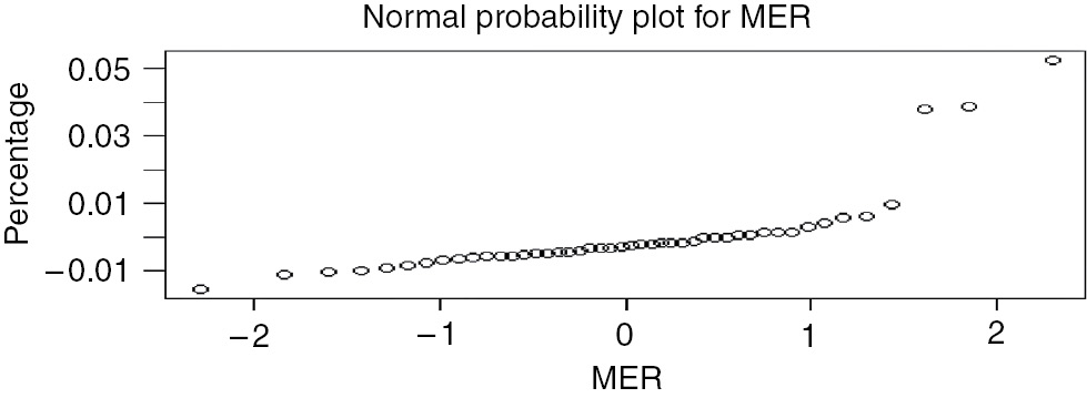
Normal Probability Plot.
Table 10 throws out a comparative statement of the models. From this table, it is clear that there is no statistically significant difference among the three models.
Comparative Model.
| Model | MMER | p-Value | r2 |
|---|---|---|---|
| MLR | 0.00189 | 0.00026 | 0.9840 |
| MNLR | 0.000574 | 0.00022 | 0.9923 |
| NN | 0.0045 | 0.00020 | 0.9820 |
5 Validation of Models
Ten out of 60 projects were set aside and used for the validation. Here again, MER and MMER were calculated. The MMER during the validation stage stood at 0.0054, 0.0016, and 0.0015 for the LRMs, non-LRMs, and neural network models, respectively. From this, it is evident that there is no statistical difference between the accuracy of prediction for the three models as the p-value is almost the same at the 95% confidence level. Figures 4–6 are the scatter plots of MER distribution for projects after validation. The visual examination of these three indicates that MER increases with the increase in the effort in the case of LRM and non-LRMs, whereas the neural network model indicated that MER remains almost at a constant level. The test of hypothesis value and p-value are also used as metrics for comparison (Table 11). It is seen from the table that p>0.05 in all the cases, suggesting that the null hypothesis for any model cannot be rejected.

MER Plot for Multiple Linear Regression.

MER Plot for Multiple Nonlinear Regression.

MER Plot for Neural Network.
Comparison of the Three Models Under Investigation.
| Model | MMER | p-Value |
|---|---|---|
| MLR | 0.00189 | 0.06 |
| MNLR | 0.000574 | 0.07 |
| NN | 0.0045 | 0.0084 |
6 Results and Discussions
The comparison of the statistical regression models, the most popular technique to date, and a machine learning model is worth considering because no single technique of effort estimation is apt for all situations. This comparison may also guide to showcase the realistic estimates. The seven parameters chosen in this work are unique and first of its kind. In both stages of verification and validation, the accuracy comparison of three models did not show a statistically significant difference. This is indicated by a very low value of the mean and median (i.e. mean and median of residues), which is presented in Table 12. The only difference is that the regression models are statistical models built on mathematical procedure, whereas the artificial neural network (ANN) is a method based on experiential learning and heuristics.
Mean and Median Distribution.
| Model | Mean | Median |
|---|---|---|
| MLR | 0.04563 | 0.0044 |
| MNLR | 0.0135 | 0.0134 |
| NN | 0.1223 | 0.1222 |
To get a clue on the relationship of the parameters and the actual effort scatter plots are presented in Figure 7A–G, the following observations could be listed:
The range of LOC 40 to 1500 seems to cluster corresponding to the range of actual effort 1000 to 2200 min.
CGPA versus actual effort clearly shows that the inversely proportional actual efforts tend to decrease with the increase in CGPA. Heralding that, the knowledge level of developer is one of the decisive factors in deciding software effort.
The actual effort seems to cluster in a range of 1000 to 2200 min for the corresponding range of N&C being in the range of 5 to 40 for all the projects.
There is a narrow range of actual effort 1000 to 2200 min for a wide range of R spanning 5 to 25.
A clustering effect is seen for CC. Most of the projects with CC are from 2 to 100 for the corresponding actual effort 1500 to 2200 min.
The algorithm complexity of Θ(n) and Θ(n2) seems to be predominant, whereas Θ(n) consumed an effort in the range of 1200–2000 min and Θ(n2) has shown an actual effort ranging from 1300 to 2500 min.
FPs in the range of 5–20 congregate for the corresponding range of actual effort 1200–2500 min.

Scatter Plots Showing Variations of Parameters with Respect to Actual Effort: (A) LOC vs. Actual Effort, (B) CGPA vs. Actual Effort, (C) N&C vs. Actual Effort, (D) RC vs. Actual Effort, (E) CC vs. Actual Effort, (F) AC vs. Actual Effort, and (G) FP vs. Actual Effort.
The observations listed above also corroborate with Pearson correlation coefficient demonstrated in Table 13. From the correlation analysis, LOC, N&C, CC, and AC have a modest direct relationship with the software effort. CGPA has an inverse relationship with the effort, whereas FP and R seem to have a marginal effect on software effort.
Pearson Correlation Coefficients Between Parameters and Actual Effort.
| Parameters | LOC | CGPA | N&C | R | CC | AC | FP |
|---|---|---|---|---|---|---|---|
| Actual effort | 0.6832 | −0.8312 | 0.7213 | 0.5612 | 0.6829 | 0.7126 | 0.4512 |
At this juncture, it is worth making a comparative analysis of similar kind of prediction models that have been recently reported.
In an attempt by Lopez-Martin et al. [21], fuzzy models have been developed for predicting software development effort for small programs. The so-developed model has also been compared to the LRM. A total of 105 small-scale programs developed by a group of 30 programers have been used in the prediction exercise. Only one input parameter (i.e. N&C) is considered. As reported in the paper, the MMER values of 0.23 for fuzzy model and 0.26 for LRM are obtained.
Further, Lopez-Martin [20] has considered GRNN for predicting software development effort for small-scale programs. For this work, the programs developed with practices based on the personal software process (PSP) were used, and samples of 163 and 80 programs were used for verification and validation, respectively. The MMER values of 0.24 and 0.31 have been obtained during verification and validation, respectively.
Yet again, Lopez-Martin et al. [22] have considered a data set obtained from the ISBSG and developed a GRNN model. Samples of 98 and 97 projects were used for verification and validation, respectively. From the results obtained from the variance analysis of accuracy, the authors have opined that the GRNN model could be an alternative to the prediction of development effort of software projects, which have been developed in industrial environments. The MMER value of 0.041 has been indicated.
From the forgone comparison, the work presented in this paper is distinct in three respects:
Unlike the state-of-the-art, the standard data set has not been used in developing the model. The input parameter and the software effort have been obtained through some kind of realistic setup. Although academic in nature, it vaguely mimicked the industry scenario.
The parameters elicited happens to be novel particularly, with references to the metrics for the knowledge level acquired by the developers (CGPA) AC and CC.
An attempt made for evolving a nonlinear multivariable regression model.
Above all, the MMER is found to be far lower in its value compared to the other reported works, suggesting the high-end accuracy of the models.
7 Conclusions
This paper presented a unique work in developing predictive models on software effort estimation with special reference to small-scale visualization projects. This work has following underpinnings:
No single software development estimation technique is apt for all kinds of software projects.
Yet, software effort estimation is considered to be most critical activity while managing software projects.
In this direction, the significant contribution of the work may be summarized as follows:
Providing reasonably accurate effort of predictive models considering pragmatic input parameters almost akin to industry project development scenario.
Evolving the hypothesis that effort prediction accuracy of multiple linear, multiple nonlinear, and ANN models are almost statically on parity.
Bibliography
[1] M. A. Ahmed, M. O. Saliu and J. Al-Ghamdi, Adaptive fuzzy logic based framework for software development effort prediction, Inf. Softw. Technol.47 (2005), 31–48.10.1016/j.infsof.2004.05.004Suche in Google Scholar
[2] Y. Ahn, J. Suh, S. Kim and H. Kim, The software maintenance projects effort estimation model based on function points, J. Softw. Mainten. Evol.15, (2003), 71–85.10.1002/smr.269Suche in Google Scholar
[3] B. Boehm, E. Horowitz, R. Madachy, D. Reifer, B. K. Clark, B. Steece, A. W. Brown, S. Chulani and C. Abts, Software Cost Estimation with Cocomo II, Prentice Hall, New Jersey, 2000.Suche in Google Scholar
[4] L. C. Briand and I. Wieczorek, Software resource estimation. Encyclopedia of software engineering, vol. 2, pp. 1160–1196, John Wiley&Sons, New York, 2001.Suche in Google Scholar
[5] C. J. Burguess and M. Lefley, Can genetic programming improve software effort estimation? A comparative evaluation, J. Inf. Softw. Technol.43 (2001), 863–873.10.1016/S0950-5849(01)00192-6Suche in Google Scholar
[6] S. D. Conte, H. E. Dunsmore and V. Y. Shen, Software engineering metrics and models, Eur. J. Oper. Res.28 (1987), 235–236.10.1016/0377-2217(87)90230-XSuche in Google Scholar
[7] F. J. Crespo, M. A. Sicicila and J. J. Cuadrado, On the use of fuzzy regression in parametric software estimation models: integrating imprecision in COCOMO cost drivers. WSEAS Trans. Syst.1 (2004), 96–101.Suche in Google Scholar
[8] I. F. De Barcelos Tronto, J. D. Simoes da Silva and N. Sant’Anna, An investigation of artificial neural networks based prediction systems in software project management, J. Syst. Softw.81 (2008), 356–367.10.1016/j.jss.2007.05.011Suche in Google Scholar
[9] I. Finschi, An implementation of the Levenberg-Marquardt algorithm, Eidgenössische Technische Hochschule, Zürich, 1996.Suche in Google Scholar
[10] A. Heiat, Comparison of artificial neural network and regression models for estimating software development effort, J. Inf. Softw. Technol.44 (2002), 911–922.10.1016/S0950-5849(02)00128-3Suche in Google Scholar
[11] W. Humphrey, A discipline for software engineering, Pearson Professional Computing, 2012.Suche in Google Scholar
[12] A. Idri, A. Abran, and L. Kjiri, COCOMO cost model using fuzzy logic, in: 7th International Conference on Fuzzy Theory&Techniques, 27 Feb–3 March, Atlantic City, NJ, 2000.Suche in Google Scholar
[13] ISO/IEC 20926:2009-IFPUG 4.1 Unadjusted functional size measurement method – counting practices manual.Suche in Google Scholar
[14] P. Jodpimai, P. Sophatsathit and C. Lursinsap, Analysis of effort estimation based on software project models, IEEE (2009).10.1109/ISCIT.2009.5341149Suche in Google Scholar
[15] M. Jørgensen, Forecasting of software development work effort: evidence on expert judgment and formal models, Int. J. Forecast.23 (2007), 449–462.10.1016/j.ijforecast.2007.05.008Suche in Google Scholar
[16] M. Jorgensen, G. Kirkeboen, D. Sjoberg, B. Anda and L. Brathall, Human judgment in effort estimation of software projects, in: International Conference on Software Engineering, Limerick, Ireland, Computacion y Sistemas, vol. 11, pp. 333–348, 2008.Suche in Google Scholar
[17] V. K. Khatibi and D. N. A. Jawawi, Software cost estimation methods: a review, J. Emerg. Trends Comput. Inf. Sci.2 (2011), 21–29.Suche in Google Scholar
[18] B. A. Kitchenham, S. L. Pfleeger, L. M. Pickard, P. W. Jones, D. C. Hoaglin, K. El Emam and J. Rosenberg, Preliminary guidelines for empirical research in software engineering, IEEE Trans. Softw. Eng.28, (2002), 721–734.10.1109/TSE.2002.1027796Suche in Google Scholar
[19] P. Kok, B. A. Kitchenhan, J. Kirakowski, The MERMAID approach to software cost estimation, in: Proceedings, ESPRIT Technical Week, 1990.10.1007/978-94-009-0705-8_21Suche in Google Scholar
[20] C. Lopez-Martin, Applying a general regression neural network for predicting development effort of short-scale programs, Neural Comput. Appl.20 (2011), 389–401.10.1007/s00521-010-0405-5Suche in Google Scholar
[21] C. Lopez-Martin, C. Yañez-Marquez and A. Gutierrez-Tornes, Predictive accuracy comparison of fuzzy models for software development effort of small programs, J. Syst. Softw.81 (2008), 949–960.10.1016/j.jss.2007.08.027Suche in Google Scholar
[22] C. Lopez-Martin, C. Isaza and A. Chavoya, Software development effort prediction of industrial projects applying a general regression neural network, J. Empir. Softw. Eng.17 (2012), 738–756.10.1007/s10664-011-9192-6Suche in Google Scholar
[23] S. G. MacDonell and A. R. Gray, Alternatives to regression models for estimating software projects, in: Proceedings of the IFPUG Fall Conference, Dallas TX, IFPUG, 1996.Suche in Google Scholar
[24] E. Mendes, N. Mosley and I. Watson, A comparison of case-based reasoning approaches to web hypermedia project cost estimation, in: Proceedings of the 11th International Conference on World Wide Web, pp. 272–280, ACM, 2002.10.1145/511446.511482Suche in Google Scholar
[25] P. Musflek, W. Pedrycz, G. Succi and M. Reformat, Software cost estimation with fuzzy models, Appl. Comput. Rev.8 (2000), 24–29.10.1145/373975.373984Suche in Google Scholar
[26] A. L. I. Oliveira, Estimation of software project effort with support vector regression, Neurocomputing69, (2005), 1749–1753.10.1016/j.neucom.2005.12.119Suche in Google Scholar
[27] B. Sigweni and M. Shepperd, Feature weighting techniques for CBR in software effort estimation studies: a review and empirical evaluation, in: Proceedings of the 10th International Conference on Predictive Models in Software Engineering, September 17–18, pp. 32–41, ACM, Turin, Italy, 2014.10.1145/2639490.2639508Suche in Google Scholar
[28] B. Sigweni, M. Shepperd and T. Turchi, Realistic assessment of software effort estimation models, in: Proceedings of the 20th International Conference on Evaluation and Assessment in Software Engineering, p. 41, ACM, 2016.10.1145/2915970.2916005Suche in Google Scholar
[29] S. Srichandan, A new approach of software effort estimation using radial basis function neural networks, Int. J. Adv. Comput. Theory Eng.1 (2012), 2319–2526.Suche in Google Scholar
[30] A. Trendowicz and R. Jeffery, Software project effort estimation: foundations and best practice guidelines for success, Springer International Publishing, 2014.10.1007/978-3-319-03629-8Suche in Google Scholar
[31] K. K. Vinay, V. Ravi, M. Carr and K. N. Raj, Software development cost estimation using wavelet neural networks, J. Syst. Softw.81 (2007), 1853–1867.10.1016/j.jss.2007.12.793Suche in Google Scholar
[32] J. Wen, S. Li, Z. Lin, Y. Hu and C. Huang, Systematic literature review of machine learning based software development effort estimation models, Inf. Softw. Technol.54 (2012), 41–59.10.1016/j.infsof.2011.09.002Suche in Google Scholar
©2018 Walter de Gruyter GmbH, Berlin/Boston
This article is distributed under the terms of the Creative Commons Attribution Non-Commercial License, which permits unrestricted non-commercial use, distribution, and reproduction in any medium, provided the original work is properly cited.
Artikel in diesem Heft
- Frontmatter
- ADOFL: Multi-Kernel-Based Adaptive Directive Operative Fractional Lion Optimisation Algorithm for Data Clustering
- A Multiple Criteria-Based Cost Function Using Wavelet and Edge Transformation for Medical Image Steganography
- Mining DNA Sequence Patterns with Constraints Using Hybridization of Firefly and Group Search Optimization
- An Approach to Detect Vehicles in Multiple Climatic Conditions Using the Corner Point Approach
- Adaptive Algorithm for Solving the Load Flow Problem in Distribution System
- Modeling and Optimizing Boiler Design using Neural Network and Firefly Algorithm
- Models for Predicting Development Effort of Small-Scale Visualization Projects
- An Effective Technique for Reducing Total Harmonics Distortion of Multilevel Inverter
- Neural Network Classifier for Fighter Aircraft Model Recognition
- Feature Selection Using Harmony Search for Script Identification from Handwritten Document Images
- A Novel Hybrid ABC-PSO Algorithm for Effort Estimation of Software Projects Using Agile Methodologies