CAT(0) cube complexes and asymptotically rigid mapping class groups
-
Marie Abadie


Abstract
The present paper contributes to the study of asymptotically rigid mapping class groups of infinitely punctured surfaces obtained by thickening planar trees.
In a paper from 2022, Genevois, Lonjou and Urech study the latter groups using cube complexes.
We determine in which cases their cube complexes are
1 Introduction
Thompson’s groups have been the subject of intense study in group theory and have proven to be a rich source of interesting examples [2, 4, 15]. They inspired the construction of other groups through variations of their concepts, called Thompson-like groups [13, 14]. Much recent work has been devoted to the study of braided versions of Thompson-like groups [3, 6], i.e. extensions of Thompson-like groups by infinite braid groups, which turn out to be closely linked to mapping class groups of surfaces of infinite type [1, 7].
Genevois, Lonjou and Urech study in [11] a particular family of braided Thompson-like groups called asymptotically rigid mapping class groups.
Their framework is inspired from [8, 9].
These groups are subgroups of big mapping class groups of infinitely punctured surfaces obtained by thickening planar trees
The cube complex
To study the case
For all
In [12], the authors suggested that it may be possible to modify their construction.
Hence we introduce a cube complex
For all
Thus we define a collection of
For all
2 Preliminaries
Let 𝐴 be a locally finite planar tree.
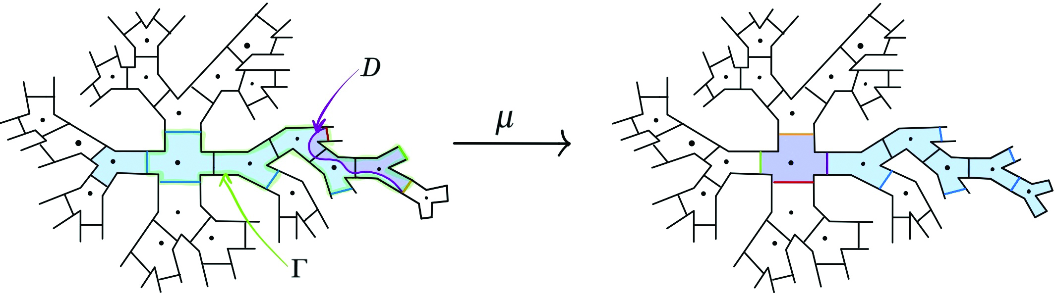
Its arboreal surface is the surface
each arc intersects one unique edge of 𝐴 and this intersection is transverse,
each polygon contains exactly one puncture in its interior.
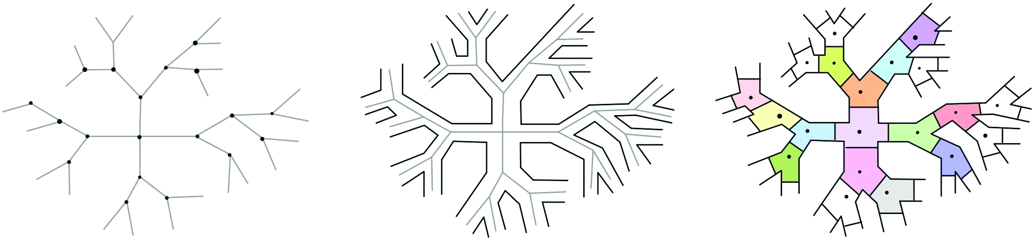
From left to right, pictures of
An admissible subsurface
An asymptotically rigid homeomorphism of
its image
outside its support
The group of isotopy classes of orientation-preserving asymptotically rigid homeomorphisms of
Funar and Kapoudjian were the first to consider the group corresponding to a regular tree of degree three and to study its generators and relations [8].
In [11], Genevois, Lonjou and Urech extend the definition to explore the finiteness properties of these groups when the tree 𝐴 is considered to be
We define an equivalence relation on the set of pairs
In [11], the authors introduce a new family of cube complexes to explore the finiteness properties of this group when the tree 𝐴 is considered to be
vertices
edges between any two vertices of the form
𝑘-cubes with underlying subgraphs of the form
where
This gives an action of
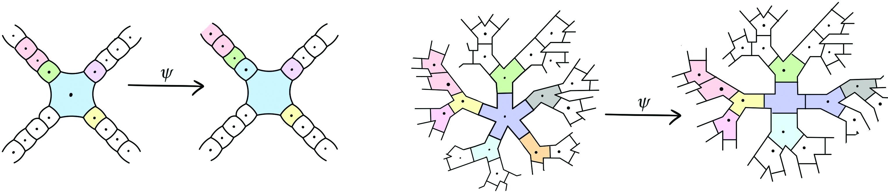
Now, let us vary the rigid structure associated to
each arc crosses once and transversely a unique edge of the tree,
each polygon contains exactly one vertex of the underlying tree in its interior. Since each vertex corresponds to a puncture except the 𝑚-valence one, each polygon contains a puncture except the central one.
its image
𝜙 sends polygons to polygons outside
There is a group isomorphism
Proof
The following argument closely follows the proof of [11, Lemma 2.4].
We fix 𝑢 to be the central vertex in

From left to right, pictures of
In the following definition, we work with the rigid structure
vertices
edges between any two vertices of the form
𝑘-cube with underlying subgraph of the form
where
Next, we present some properties about
Lemma 2.2 ([11, Lemma 3.4])
Let
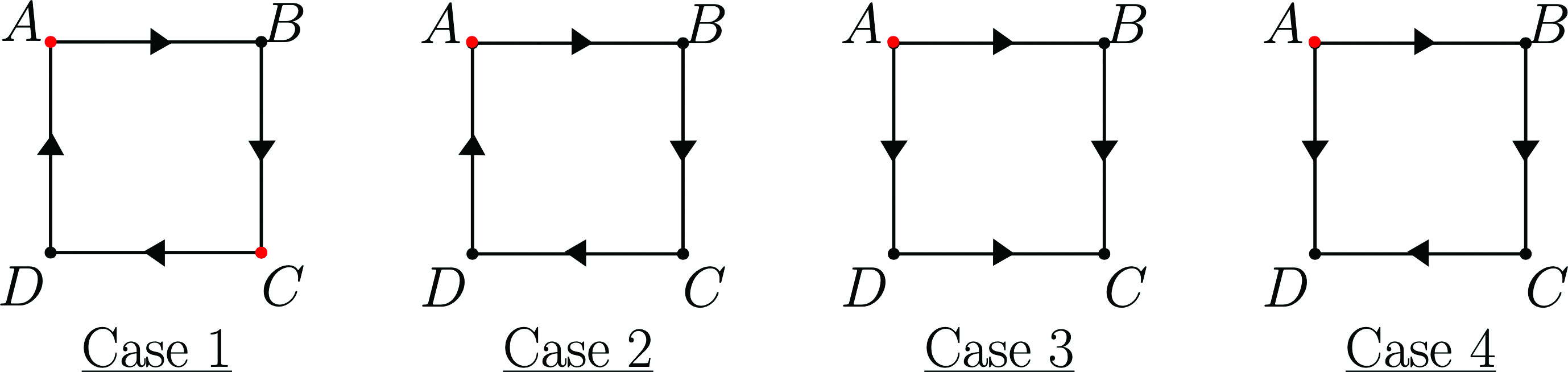
The height orientation is obtained by giving an orientation to all the edges of
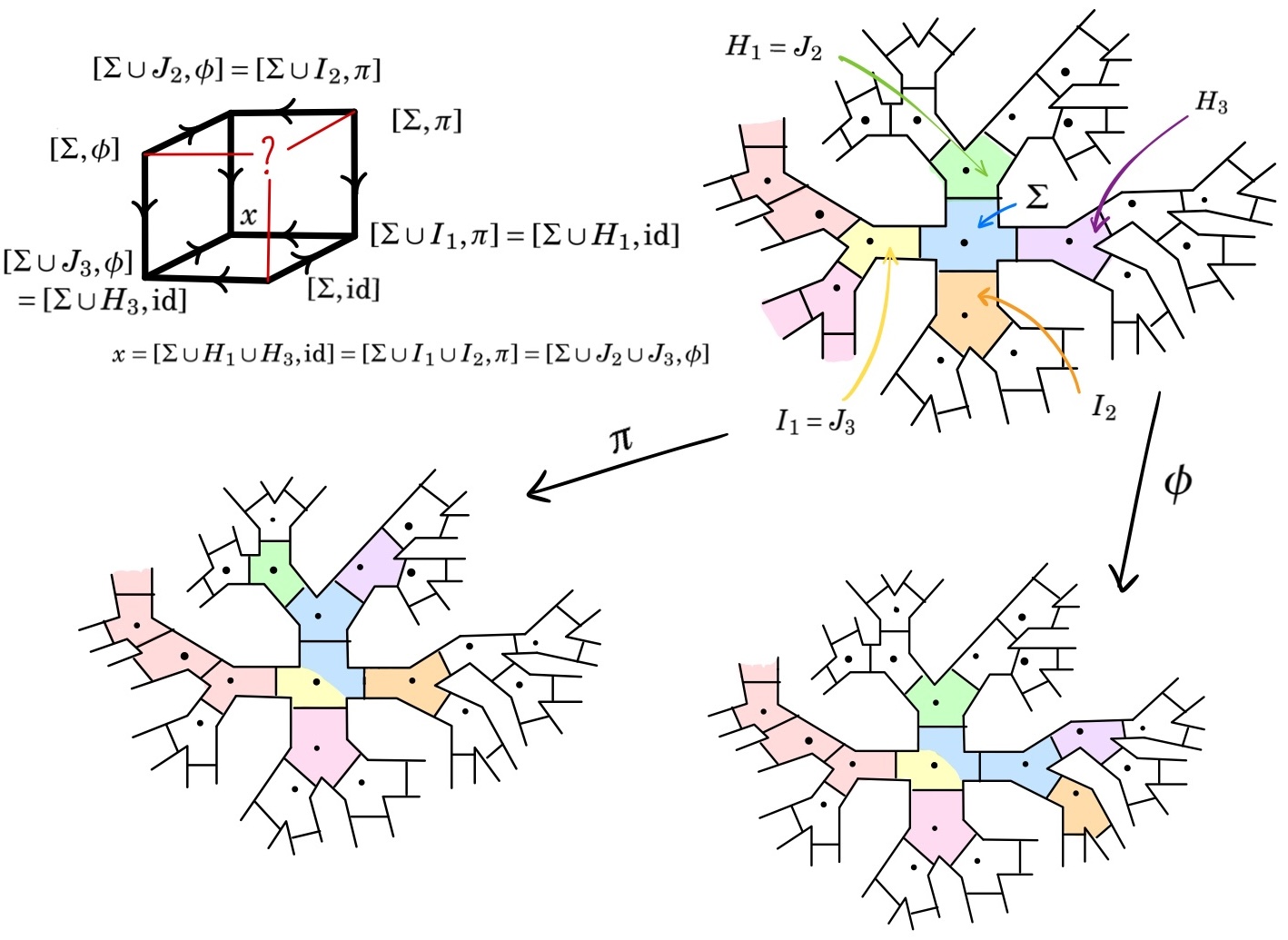
Let 𝑆 be a 2-cube in
Proof
We work with
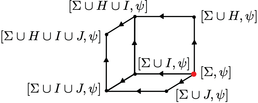
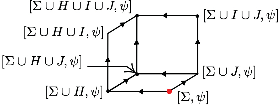
Any 3-cube must have a specific orientation with respect to the height function.
In particular, it must have one smallest vertex 𝑥, then three vertices of height
Let Γ be a graph; its cube-completion
Let
Proof
We work with
for some admissible surface Σ, an asymptotically rigid homeomorphism 𝜙, and distinct polygons
We label the vertices of 𝑆 by bit strings
Proof of the claim
We show this by induction on 𝑛.
For
Pick a vertex in 𝑆 with minimal height and give it the label
In particular, all the neighbours of
Fix a labelling of the vertices of 𝑆 as in the above claim.
By Lemma 2.2, the 𝑛 neighbours of
Now, the vertices with exactly two 1’s in their label are also determined by the above.
For example, the vertex with 1’s in entries 𝑖 and 𝑗 must have the form
3 Studying the CAT(0)-ness of the cube complexes
C
(
A
n
,
m
)
and
D
(
A
n
,
m
)
In the first part of this section, we derive some properties on
Recall that a cube complex is said to be
The next proposition provides a tool to show that a cube complex is
Let 𝑋 be a connected graph. Assume that
the cube completion
𝑋 has no 1-corner,
𝑋 does not contain a copy of the complete bipartite graph
By definition, for all
There is no copy of the bipartite graph
Proof
We work with
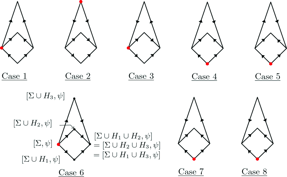
By Lemma 2.3, it remains to study Case 6.
We mark with a red dot the vertices from which all incident edges point outwards.
Let us assume the red point is
3.1 Completing roots of 3-corners
In this subsection, we study the 3-cube condition in
Every 3-corner in
Proof
We consider

Consider Case 1 in Figure 6.
In this case, there is only one red point written as
completes the 3-corner into a 3-cube.
Here we consider Case 2 in Figure 6.
There is only one red point which can be written as
For the third case in Figure 6, we proceed in the same way as above.
Assume that the red point is
The vertex
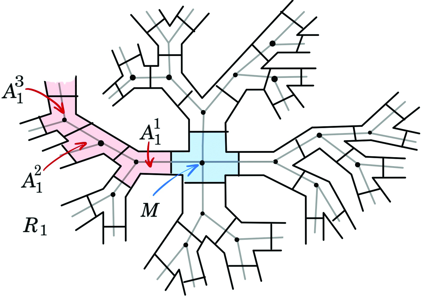
In this section, we denote by 𝑀 the central polygon in
Our last goal in this subsection is to show the following proposition.
If
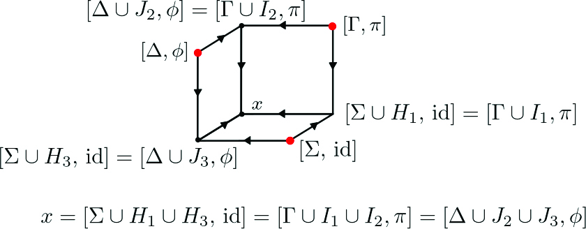
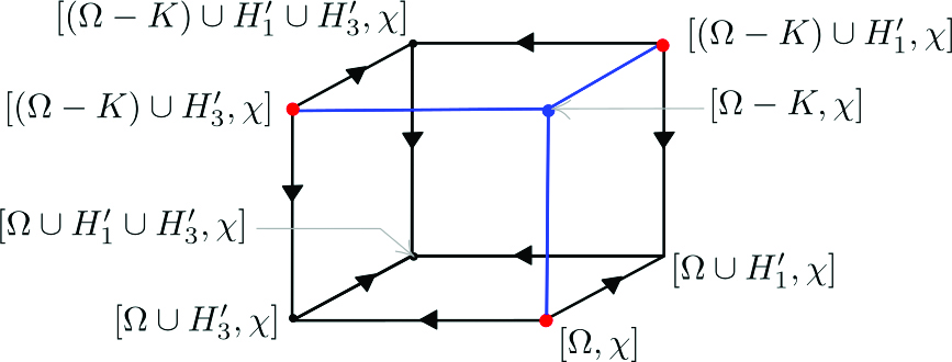
The following facts can be deduced from the equalities associated with each vertex in Figure 7:
We need the four following lemmata to prove Proposition 3.4.
Assume that we are in the situation of a 3-corner with an attracting root in
Proof
We use the same notation as depicted in Figure 7.
On one hand, by facts iii and vi, we deduce that
The polygon
Consider a 3-corner with an attracting root in
Let 𝑥 be a vertex with minimal height in a 3-corner with an attracting root in
Let Σ be an admissible surface in
Let
Proof
Consider a 3-corner with an attracting root in
First, we assume that
Hence (3.1) becomes
Both cases imply directly that
Secondly, we assume that
Under our assumptions, this equality becomes
So if
Assume
so
Assume Σ contains 𝑀. By iii and vi,
Let
Let Σ be an admissible surface in
if 𝐷 contains
and
Proof
Let Σ be an admissible surface in
Consider a 3-corner with an attractive root whose minimum vertex height is at least 2. Assume that we are in one of the following situations:
Proof
Consider a 3-corner with an attracting root and the notation as in Figure 7.
Assume that we are in one of the situations described by the assumptions of the statement; in particular,
Recall that, in the case of a 3-corner with an attracting root,
where
Assume that 𝐷 contains 𝑚 frontier arcs. If
where
Proof of Proposition 3.4
Consider a 3-corner with an attracting root and the notation as in Figure 7.
Let
First assume that
either
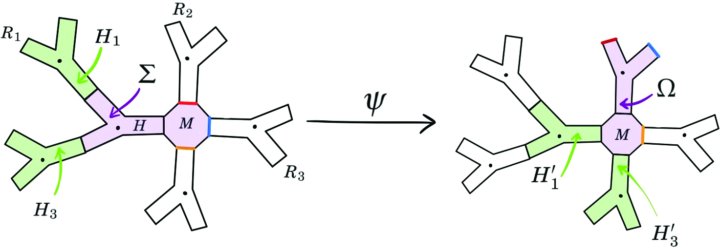 Figure 10
Or
Secondly, assume that
Thirdly, let
where
3.2 When is
C
(
A
n
,
m
)
a CAT(0) cube complex?
In this section, we determine for which subfamilies of
The cube complexes
As noted in [11],
Consider the cube complex
For
Fix three infinite rays of polygons
If
Proof
Let
For the converse, let
Let
3.3 CAT(0)-ness of the cube complex
D
(
A
n
,
m
)
First, we show that
Lemma 3.16 ([11, Claim 3.6])
Let 𝒮 be a finite collection of vertices in
Proof
Let
For the next lemma, the proof follows the same steps as in [11, Section 3.2], where the case of
Let 𝒮 be a finite collection of vertices in
Proof
Let 𝒮 be a finite collection of vertices in
where Δ is an admissible surface and
The cube generated by the vertices
Proof of the claim
One has a height-increasing path from 𝑥 to
so
In particular, all the direct neighbours
This sequence stops since
If
Proof
Let
Let
Proof
Let
Now, we define the collection of cube complexes
For all
Proof
Let
now the latter group acts on
Funding source: Fonds National de la Recherche Luxembourg
Award Identifier / Grant number: O19/13865598
Funding statement: This work was partially supported by the Luxembourg National Research Fund OPEN grant O19/13865598.
Acknowledgements
The main part of this work was carried out in the context of a master’s thesis under the supervision of Christian Urech who provided the main question, guidance and a friendly environment. We thank the referee for the comments and suggestions that helped us to improve the clarity of the presentation.
-
Communicated by: Rachel Skipper
References
[1] J. Aramayona and N. G. Vlamis, Big mapping class groups: An overview, In the Tradition of Thurston—Geometry and Topology, Springer, Cham (2020), 459–496. 10.1007/978-3-030-55928-1_12Search in Google Scholar
[2] J. M. Belk, Thompson’s group F, Ph.D. Thesis, Cornell University, 2007. Search in Google Scholar
[3] M. G. Brin, The algebra of strand splitting. I. A braided version of Thompson’s group 𝑉, J. Group Theory 10 (2007), no. 6, 757–788. 10.1515/JGT.2007.055Search in Google Scholar
[4] J. W. Cannon, W. J. Floyd and W. R. Parry, Introductory notes on Richard Thompson’s groups, Enseign. Math. (2) 42 (1996), no. 3–4, 215–256. Search in Google Scholar
[5]
V. Chepoi,
Graphs of some
[6] P. Dehornoy, The group of parenthesized braids, Adv. Math. 205 (2006), no. 2, 354–409. 10.1016/j.aim.2005.07.012Search in Google Scholar
[7] L. Funar, Braided Houghton groups as mapping class groups, An. Ştiinţ. Univ. Al. I. Cuza Iaşi. Mat. (N.S.) 53 (2007), no. 2, 229–240. Search in Google Scholar
[8] L. Funar and C. Kapoudjian, The braided Ptolemy–Thompson group is finitely presented, Geom. Topol. 12 (2008), no. 1, 475–530. 10.2140/gt.2008.12.475Search in Google Scholar
[9] L. Funar, C. Kapoudjian and V. Sergiescu, Asymptotically rigid mapping class groups and Thompson’s groups, Handbook of Teichmüller Theory. Volume III, IRMA Lect. Math. Theor. Phys. 17, European Mathematical Society, Zürich (2012), 595–664. 10.4171/103-1/11Search in Google Scholar
[10] A. Genevois, Algebraic properties of groups acting on median graphs, 2022. Search in Google Scholar
[11] A. Genevois, A. Lonjou and C. Urech, Asymptotically rigid mapping class groups, I: Finiteness properties of braided Thompson’s and Houghton’s groups, Geom. Topol. 26 (2022), no. 3, 1385–1434. 10.2140/gt.2022.26.1385Search in Google Scholar
[12] A. Genevois, A. Lonjou and C. Urech, Asymptotically rigid mapping class groups, II: Strand diagrams and nonpositive curvature, preprint (2021), https://arxiv.org/abs/2110.06721; to appear in Trans. Amer. Math. Soc. Search in Google Scholar
[13] G. Higman, Finitely Presented Infinite Simple Groups, Notes Pure Math. 8, Australian National University, Canberra, 1974. Search in Google Scholar
[14] S. R. Lee, Geometry of Houghton’s groups, Ph.D. Thesis, The University of Oklahoma, 2012. Search in Google Scholar
[15] E. T. Shavgulidze, The Thompson group 𝐹 is amenable, Infin. Dimens. Anal. Quantum Probab. Relat. Top. 12 (2009), no. 2, 173–191. 10.1142/S0219025709003719Search in Google Scholar
© 2024 the author(s), published by De Gruyter
This work is licensed under the Creative Commons Attribution 4.0 International License.
Articles in the same Issue
- Frontmatter
- On the kernel of actions on asymptotic cones
- CAT(0) cube complexes and asymptotically rigid mapping class groups
- Iwip endomorphisms of free groups and fixed points of graph selfmaps
- Space of orders with finite Cantor–Bendixson rank
- Lifting subgroups of PSL2 to SL2 over local fields
- Regular 3-polytopes of order 2𝑛𝑝
- On the number of tuples of group elements satisfying a first-order formula
- Exponent-critical groups
- On soluble groups in which commutators have prime power order
- A character theoretic criterion for Fitting height
- Hilbert divisors and degrees of irreducible Brauer characters
- Character triples and relative defect zero characters