New Traffic Conflict Measure Based on a Potential Outcome Model
-
 and
and

Abstract
A key issue in the analysis of traffic accidents is to quantify the effectiveness of a given evasive action taken by a driver to avoid crashing. Since 1977, the widely accepted definition for this effectiveness measure, which is called traffic conflict, has been “the risk of a collision if the driver movement remains unchanged.” Although the definition is expressed counterfactually, the full power of counterfactual analysis was not utilized. In this paper, we propose a counterfactual measure of traffic conflict called Counterfactual Based Conflict (CBC). The CBC is interpreted as the probability that a driver avoided a crash actually by taking an evasive action in the counterfactual situation in which the crash would have occurred if he/she had not taken an evasive action and the crash would not have occurred if he/she had taken an evasive action. The CBC captures realistic aspects of the traffic situation, and lends itself to modern causal analysis. In addition, we provide some of identification conditions for the CBC. Furthermore, we formulate bounds on the CBC when the proposed identification conditions are violated. Finally, through an application of the CBC to the 100-Car Naturalistic Driving Study, we discuss the usefulness and limitations of the proposed measure.
1 Introduction
A traffic crash occurs when one vehicle collides with another vehicle or with a pedestrian, animal, road debris, or other stationary obstruction such as a tree or utility pole and often leads to severe consequences, including injury, death and property damage [1], [2], [3]. With the aim of preventing such consequences, a great deal of research effort has been expended in developing road safety theory (i. e., why crashes occur?), and identifying factors affecting road safety (i. e., what caused crashes?) [2], [4], [5].
It would be reasonable to observe crashes to conduct successful road safety research, if such observation were possible. However, there are two difficulties in conducting such research. First, crashes occur sporadically, and some of them might not be reported [6]. Second, waiting for such severe consequences in order to prevent crashes is questionable ethically [7]. To overcome these drawbacks, Perkins and Harris [8] developed a traffic conflict technique that analyzes observed situations in which drivers took an evasive action to avoid crashes.
Since the seminal work of Perkins and Harris [8], the concept of traffic conflicts has been refined and discussed by many researchers and practitioners in the field of road safety research [9], [10], [11]. In Oslo in 1977, a conceptual definition of traffic conflicts was proposed in the first workshop on traffic conflicts. The definition, which has been widely accepted by road safety researchers and practitioners since then, is as follows:
“A traffic conflict is an observable situation in which two or more road users approach each other in space and time to such an extent that there is a risk of collision if their movements remain unchanged” [12].
Regarding this definition, Davis et al. [13] pointed out that
“An observed event qualifies as a conflict only if it satisfies a counterfactual test; if the movements had remained unchanged then a collision would probably have resulted,”
and introduced the idea of counterfactual conditionals on the basis of structural causal model [14] into traffic conflict technique [13], [15], [16].
In 1982, Hauer [17] pointed out the importance of crash-to-conflict ratio in the traffic conflict technique. Since then, over the past decades, the research on crash-to-conflict ratio has attracted interest in the field of traffic conflict technique. Recently, Davis et al. [13] proposed a novel type of crash-to-conflict ratio based on the level of initial conditions in traffic situations and clarified some of the properties. We refer to this crash-to-conflict ratio as “Davis’s crash-to-conflict ratio.” Different from the existing traffic conflict techniques, Davis’s crash-to-conflict ratio is formulated based on the conceptual aspect of the potential outcomes in the form of the initial conditions. Although it is assumed that the information on the initial conditions are fully available in Davis et al. [13], considering that crashes occur as a result of complex interactions among drivers, their vehicles, and their road environments [7], it would be reasonable to consider that the initial conditions cannot be observed fully in actual field studies. Thus, it might be unrealistic to evaluate Davis’s crash-to-conflict ratio under such an assumption. Solving this problem requires formulating a new traffic conflict measure.
This paper proposes a new traffic conflict measure, the Counterfactual Based Conflict (CBC). To overcome the drawback of existing traffic conflict techniques, the CBC is formulated based on the potential outcome model, and thus reflects the counterfactual statement. The CBC can be interpreted as the probability that a driver avoided a crash actually by taking an evasive action in the counterfactual situation in which the crash would have occurred if he/she had not taken an evasive action and the crash would not have occurred if he/she had taken an evasive action. In this sense, the CBC evaluates the effectiveness of a given evasive action to avoid crashing, that is, the rate at which drivers in the abovementioned counterfactual situation actually avoided crashes by taking an evasive action. In addition, we provide identification conditions for the CBC. Furthermore, we formulate the bounds on the CBC, that is, the ranges within which the true values of the CBC must lie, when the proposed identification conditions are violated. Finally, through an application of the CBC to the 100-Car Naturalistic Driving Study (hereafter, the 100-car study) [1], we discuss the usefulness and limitations of the proposed measures. The extension of the CBC to a case of multiple evasive actions is also discussed in Appendix.
2 Potential outcome model
In this section, we introduce the potential outcome model [14], [18], [19], [20], to propose our new traffic conflict measure.
Let X and Y be random variables indicating an evasive action of a driver and a collision-related outcome, respectively. For simplicity, regarding a dichotomous evasive action X,
A collision-related outcome Y is the consequence of an evasive action taken in the event of interest, such as a crash or a near crash defined by physical quantities (e. g., the distance between vehicles and the time required for two vehicles to collide). Thus, Y can be a variable that takes a sampled value over time such as the time to collision (TTC), or a properly selected single value such as the minimum TTC or the time gap. The selection of the collision-related outcome depends on the problem setting of interest. Although it is important to develop a protocol to observe the collision-related outcome, we do not focus on this because the discussion in the paper does not depend on a specific accident occurrence process. For the discussion of the protocol to observe the collision-related outcome, for example, refer to Brown [21], Hayward [22], and Van der Horst and Hogema [23] for the TTC, and refer to Sun and Benekohal [24] for the time gap.
When
Regarding the ith of the N drivers, for
Note that neither the “no multiple versions of treatment” nor the “consistency” assumption is required in the framework of structural causal models [14]. They are derived from the assumption of autonomous data-generating process. Davis et al. [13] addressed structural causal models that represent collision-related outcomes resulting from interactions between initial conditions and evasive actions. Here, our results can also be derived in the framework of structural causal models, because the potential outcome can be constructed from structural causal models [14].
When a randomized experiment is conducted, X is independent of
Here, “identifiable” means that the causal quantities such as
Here,
3 Counterfactual Based Conflict (CBC)
3.1 Definitions and basic properties
Letting U be the set of discrete and continuous variables representing driver conditions that could affect X and Y, both observed and unobserved, Davis et al. [13] described the causal mechanism of a collision-related outcome Y in terms of the directed graph shown in Fig. 1. In Davis et al. [13], a condition U is limited to the running status of vehicles (e. g., speed, deceleration, headway, and driver reaction time). In contrast, in this paper, condition U is not so limited but covers any factor necessary to make
where
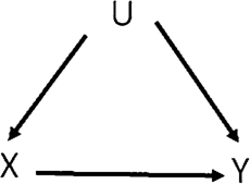
Simple graphical representation of the causal mechanism of a collision-related outcome.
In the situation shown in Fig. 1, irrespective of the complexity of U, the impact of U on Y cannot amount to more than a modification of the functional relationship between X and Y. Thus, for example, letting Y be a dichotomous variable based on a threshold y, there are exactly four functions regarding two dichotomous variables X and Y, and thus the value taken by U selects one of these four functions [14], [36]. Considering these observations, based on the level of an evasive action X, Davis et al. [13] divided driver conditions into the following four types:
is the “safe condition” in which a driver would not have crashed regardless of the level of an evasive action. In this paper, we call a driver who satisfies this condition “a safe driver” for simplicity.
is the “normal condition” in which a driver would not have crashed if he/she had taken an evasive action and would have crashed if he/she had not taken an evasive action. We call a driver who satisfies this condition “a normal driver.”
is the “doomed condition” in which a driver would have crashed regardless of the level of an evasive action. We call a driver who satisfies this condition “a doomed driver.”
is the “incompetent condition” in which a driver would have crashed if he/she had taken an evasive action and would not have crashed if he/she had not taken an evasive action. We call a driver who satisfies this condition “an incompetent driver.”
As seen from Eq. (2), the CBC is the probability that a normal driver took an evasive action and did not crash actually. Here,
Davis et al. [13] pointed out two features of the definition of traffic conflicts:
“First, the situation referred to appears to have three components: an initial condition, the actions of the road users, and a collision-related outcome. Second, an observed event qualifies as a conflict only if it satisfies a counterfactual test.”
In Eq. (2), the initial condition is given by
According to Davis et al. [13],
For a dichotomous variable X, since
Here,
is the probability that a normal driver crashed actually. This is also interpreted as the special case of “the crash-to-conflict ratio for initiating events in set
Eqs. (3) and (4) show that the probability that a normal driver took an evasive action actually is equivalent to the probability that he/she did not crash actually, as Davis et al. [13] pointed out.
Guttinger [41] stated,
“For some, the conflict is an event that precedes an evasive action that can be either successful or not (collision). For others, it is the same as a near-miss situation after an evasive action. In this last view, a conflict cannot lead to a collision but is an event parallel with a collision.”
Regarding Guttinger’s statement, the CBC probabilistically evaluates the second interpretation in the sense that it takes an actual evasive action into account. Here, although the word “traffic conflict” implies Guttinger’s first interpretation in some existing studies, this paper uses the word in the sense of Guttinger’s second interpretation that includes both crash and near-miss situations. The term “near-miss” used in Guttinger’s statement is considered to be the same as the concept of “near crash” in this paper.
As for Guttinger’s first interpretation, letting Z be a set of covariates not affected by evasive action X, we can also propose a traffic conflict measure,
which includes the ratio between the PNS,
It is worth emphasizing that the use of the CBC becomes significant when we wish to judge the effectiveness of an evasive action. For a crash that would have occurred if a driver had not taken an evasive action, the CBC evaluates the extent to which the crash was avoided by taking an evasive action actually. A higher value of the CBC suggests that an evasive action actually taken by a driver was more effective in avoiding the crash, represented by the given value y. In addition, the CBC is associated with the probability of the crash
Therefore, when the value of the CBC is higher, the probability of the crash may be lower. This implies that the use of the CBC with a continuous collision-related outcome enables us to evaluate the effectiveness of an evasive action to avoid a severe consequence at any level.
The CBC is defined based on normal drivers, but we can also focus on other conditions to formulate “CBC-like measures” if necessary. For example, regarding safe drivers, doomed drivers, and incompetent drivers, the “CBC-like measures” that we can consider are
and the conditional CBC-like measures as
3.2 Identification conditions
Since the CBC is adapted from Davis et al. [13], when incompetent drivers do not exist in the population of interest, the CBC would be identifiable if we derive the information stated in Davis et al. [13]: (i) a structural model of crash events that supports counterfactual situation, (ii) understanding how evasive actions are achieved over a range of conflict severities, and (iii) knowledge of the relative frequencies of the different conflict severities. However, it may be difficult to derive such information in reality. In addition, the CBC is formulated on the basis of the joint distributions of potential outcomes
Proposition 1.
Assume that the whole population consists only of normal drivers for a given y (i. e.,
The proof is straightforward from Eqs. (3) and (4).
Perkins and Harris [8] stated that
“Over 20 objective criteria for traffic conflicts (or impending accident situations) have been defined as to specific accident patterns at intersections. Essentially, these traffic conflicts are defined by the occurrence of an evasive action, such as braking or weaving, which are forced on a driver by an impending accident situation or a traffic violation.”
Eq. (14) implies that the concept of traffic conflicts proposed by Perkins and Harris [8] does not contradict the counterfactual statement given at the first workshop on traffic conflicts. In addition, Eq. (15) implies that the concept of traffic conflicts defined by collision-related outcomes such as the TTC is justified when the population under consideration consists only of normal drivers.
From Proposition 1, when both
This property is useful for supporting the hypothesis that the population under consideration includes various types of drivers through the use of statistical data. Consider the statistical hypothesis
If the null hypothesis
Proposition 2.
Assume that
The proof is straightforward from Eq. (4).
Proposition 3.
Assume that incompetent drivers do not exist in the population under consideration. If
The proof can be achieved as a special case of Proposition 8 in Appendix A.
We assume that
3.3 Bounds
As can be seen from the definition, the CBC is not identifiable based on the knowledge of observed data alone, even under the conditional ignorability condition. When the CBC is not identifiable, one possible solution is to derive the closed-form formulas of the bounds on the CBC under the milder conditions.
Proposition 4.
Assume that
The proof can be achieved as a special case of Proposition 9 in Appendix A.
Intuitively, Eq. (18) implies that drivers who took an evasive action actually in the normal condition are more numerous than both those in the safe condition and those in the doomed condition. In addition, Eq. (19) shows that doomed drivers are more numerous than safe drivers in the population of interest. These assumptions would be reasonable when we focus on a traffic situation such as a potential rear-end collision in which a driver of the following vehicle adequately recognizes the risk of crashing. Note that Eq. (18) or Eq. (19) might not hold for specific values of y. In this case, the lower bound on the CBC is undefined. In this context, the assumption in Eq. (18) may be thought questionable when y is close to zero. However, Eq. (18) would still be reasonable when the main focus is on traffic safety research with a categorized collision-related outcome as, for example, in the 100-car study discussed in Section 4.
Proposition 5.
If both
Proposition 5 can be proved as a special case of Proposition 10 in Appendix A.
4 Application to the 100-car study
4.1 Background
We apply the proposed traffic conflict measure to the data from the 100-car study, as shown in Table 1. The data was collected by the National Highway Traffic Safety Administration, Virginia Department of Transportation, and Virginia Tech Transportation Institute over a period of more than a year, from January 2003 to July 2004, from 100 drivers, to observe their behavior in various traffic situations that arise in daily life. The drivers were recruited through a newspaper advertisement. Thus, the 100-car study was an observational study.
According to Dingus et al. [1], first, events of interest that are candidate collision-related outcomes were selected based on the sensing values of lateral acceleration, longitudinal acceleration, forward TTC, rear TTC, yaw rate, and event button. The thresholds of these values were determined from a sensitivity analysis. Invalid events were then excluded by trained operators, whom Dingus et al. [1] referred to as “data reductionists.” They took account of the following: (a) video data on the driver’s view and behavior, and (b) time plots of the sensing values. They also assigned each valid event (i. e., collision-related outcome) to one of three levels: crash
4.2 Analysis
Based on the data provided in Table 1, we present an analysis of rear-end collisions by the following vehicles. In Table 1, “evasive action (
Note that
Drivers of the following vehicles: dichotomous evasive action.
| Crash | Near crash | Incident | |
| No evasive action | 7 | 0 | 29 |
| Evasive action | 8 | 380 | 5754 |
From Table 1, the unbiased estimates of
Here, regarding
5 Conclusions
In recent road safety studies, researchers and practitioners have proposed a range of traffic conflict techniques. However, most of these did not consider the counterfactual statement “there is a risk of collision if their movements remain unchanged.” To address this, we have proposed a new traffic conflict measure, the CBC. In contrast with most existing traffic conflict techniques, the CBC is formulated based on the potential outcome model in causal inference; hence, reflecting the counterfactual statement. We also provided identification conditions for the CBC and formulated the bounds on the CBC under particular assumptions when the proposed identification conditions are violated. In addition, through an application to the 100-car study, we showed that the CBC is helpful in reliably evaluating the effectiveness of an evasive action.
Funding source: Japan Society for the Promotion of Science
Award Identifier / Grant number: 15K00060
Funding statement: This work was partially supported by Japan Society for the Promotion of Science (JSPS), Grant Number 15K00060.
Acknowledgment
We would like to thank Professor Christer Hyden of Lund University and Clemens Kaufmann of International Co-operation on Theories and Concepts in Traffic Safety for providing us with important literature. In addition, we would like to appreciate comments from two referees that significantly improved the presentation of the paper. Finally, we thank Professor Judea Pearl of UCLA for his suggestion about clarifying emphasis points of the paper.
Appendix A CBC with multiple evasive actions
The occurrence of a crash depends not only on whether or not a driver takes an evasive action but also on what type of evasive action is taken. To address this issue, we discuss the case in which a driver chooses one of a set of possible evasive actions
A.1 Identification conditions and bounds
In this section, we provide the identification conditions and bounds for the CBC with multiple evasive actions. The proofs are given in the Appendix D.
Proposition 6.
Assume that
Proposition 7.
Assume that
Proposition 8.
Assume that
Proposition 9.
Assume that
Proposition 10.
If both
Appendix B Application to the 100-car study (CBC with multiple evasive actions)
Here, we apply the results from the CBC with multiple evasive actions in Appendix A to the rear-end collision data from the 100-car study. According to Dingus et al. [1], we classified evasive actions into four types. “Ordinary evasive action (
Drivers of the following vehicles: multiple evasive actions.
| Crash | Near crash | Incident | |
| No evasive action | 7 | 0 | 29 |
| Ordinary evasive action | 6 | 265 | 4930 |
| Aggressive evasive action | 1 | 111 | 746 |
| Skilled evasive action | 0 | 4 | 69 |
Based on Table 2, we address whether the following equation from Proposition 6 is reasonable to hold for
Here, in Table 3, under the assumption that Table 2 is generated from a multinomial distribution, we provide some statistics derived from Table 2. In Table 3, the first and second rows show the unbiased estimates and the standard error of the corresponding probabilities, respectively.
Unbiased estimates and standard errors.
| No evasive action | 0.0058 | 0.0047 | 0.0047 |
| (0.0010) | (0.0009) | (0.0009) | |
| Ordinary evasive action | 0.8432 | 0.8423 | 0.7993 |
| (0.0046) | (0.0046) | (0.0051) | |
| Aggressive evasive action | 0.1391 | 0.1389 | 0.1209 |
| (0.0044) | (0.0044) | (0.0042) | |
| Skilled evasive action | 0.0118 | 0.0118 | 0.0112 |
| (0.0014) | (0.0014) | (0.0013) |
Table 3 indicates that there appears to be no strong reason for
In contrast, since there appear to be significant differences between
Lower bounds on the CBCs.
| – | 0.3332 | 0.3324 | 0.3230 | |
| – | (0.0001) | (0.0003) | (0.0040) | |
| 0.3332 | – | 0.3326 | 0.3244 | |
| (0.0001) | – | (0.0003) | (0.0037) | |
| 0.3323 | 0.2973 | – | 0.3318 | |
| (0.0004) | (0.0023) | – | (0.0015) | |
| 0.3224 | 0.1444 | 0.2163 | – | |
| (0.0043) | (0.0111) | (0.0117) | – |
The results in Table 4 indicate that the lower bounds on
Appendix C Numerical examples
In this appendix, we present comparisons of the CBC and
Here,
In accordance with previous empirical studies [24], [51], we assume that the collision-related outcomes follow the Weibull distribution with a shape parameter of approximately 1.0∼2.5. With such a parameter setting, the marginal distribution of Eq. (39) has a unimodal right-skewed shape with a long right tail. In addition, regarding the scale parameters, a smaller value given

Comparison between the CBC and
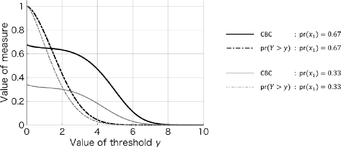
Comparison between the CBC and
Here, although we compare the CBC and
First, based on observations from the empirical studies, letting
we show the difference between the CBC and
Next, letting
Fig. 3 shows the difference between the CBC and

CBC and bounds (when
Finally, Fig. 4, which was obtained using the same parameter settings that were used to generate Fig. 2, shows the function shapes of the CBC and Eq. (20). In the figure, the lower bound on the CBC is a decreasing function of y, and the lower bound is smaller than the CBC. Here, the lower bound is undefined when y is smaller than 1.690 and larger than 5.190 because the proposed assumptions in Proposition 4 do not hold.
Appendix D Proofs
Proofs of Propositions6and7. Note that
Thus, when
Proof of Proposition8. When
Proof of Proposition9. First, we show that the following equation can be obtained:
To do this, from Eqs. (33) and (34), we derive
Then, from Eq (35), we derive
Thus, we have
which leads to Eq. (41).
Second, we show that the following equation can be obtained:
To do this, we derive
From Eq. (33), the first term of Eq. (43) can be transformed into
And from Eq. (41), the third term of Eq. (43) can be transformed into
By combining these equations, we derive Eq. (42). Since the CBC with multiple evasive actions can be transformed into
from Eq. (42), we have Eq. (36).
Proof of Proposition10. From Eq. (43), the CBC can be transformed as follows:
This leads to Eq. (37) by considering bounds on probabilities of causation (i. e.,
References
1. Dingus TA, Klauer SG, Neale VL, Petersen A, Lee SE, Sudweeks J, Perez MA, Hankey J, Ramsey D, Gupta S, Bucher C, Doerzaph ZR, Jermeland J, Knipling RR. The 100-car naturalistic driving study: phase II – results of the 100-car field experiment. DOT, HS-810 2006;593.10.1037/e624282011-001Search in Google Scholar
2. Traffic Accident Causation in Europe (TRACE) project. All TRACE reports are available for download at http://www.trace-project.org, 2006–2008.Search in Google Scholar
3. Zheng L, Ismail K, Meng X. Traffic conflict techniques for road safety analysis: open questions and some insights. Can J Civ Eng. 2014;41:633–41.10.1139/cjce-2013-0558Search in Google Scholar
4. Theofilatos A, Yannis G. A review of the effect of traffic and weather characteristics on road safety. Accid Anal Prev. 2014;72:244–56.10.1016/j.aap.2014.06.017Search in Google Scholar
5. Wang C, Quddus MA, Ison SG. The effect of traffic and road characteristics on road safety: a review and future research direction. Saf Sci. 2013;57:264–75.10.1016/j.ssci.2013.02.012Search in Google Scholar
6. Parker MR, Zegger CV. Traffic conflict techniques for safety and operations: observers manual. Federal Highway Administration. FHWA–IP–88–027 1989.Search in Google Scholar
7. Chin HC, Quek ST. Measurement of traffic conflicts. Saf Sci. 1997;26:169–85.10.1016/S0925-7535(97)00041-6Search in Google Scholar
8. Perkins SR, Harris JI. Traffic conflict characteristics: accident potential at intersections. General Motors Research Publication. GMR–718 1967.Search in Google Scholar
9. Hyden C. The development of a method for traffic safety evaluation: the Swedish traffic conflict technique. Lund Institute of Technology, Department of Traffic Planning and Engineering, Doctoral Thesis 1987.Search in Google Scholar
10. Migletz DJ, Glauz WD, Bauer KM. Relationships between traffic conflicts and accidents volume 2: final technical report. Federal Highway Administration. FHWA/RD–84/042 1985.Search in Google Scholar
11. Spicer BR. Study of traffic conflicts at six intersections. TRRL Report LR551. 1973.Search in Google Scholar
12. Amundsen FH, Hyden C. Proceedings of the First Workshop on Traffic Conflicts. Oslo; 1977.Search in Google Scholar
13. Davis GA, Hourdos J, Xiong H, Chatterjee I. Outline for a causal model of traffic conflicts and crashes. Accid Anal Prev. 2011;43:1907–19.10.1016/j.aap.2011.05.001Search in Google Scholar
14. Pearl J. Causality: models, reasoning, and inference. 2nd ed. Cambridge University Press; 2009.10.1017/CBO9780511803161Search in Google Scholar
15. Davis GA. Using Bayesian networks to identify the causal effect of speeding in individual vehicle/pedestrian collisions. In: Proceedings of the 17th Conference on Uncertainty in Artificial Intelligence. 2001. p. 105–11.Search in Google Scholar
16. Davis GA. Towards a unified approach to causal analysis in traffic safety using structural causal models. In: Transportation and Traffic Theory in the 21st Century. 2002. p. 247–65.10.1108/9780585474601-013Search in Google Scholar
17. Hauer E. Traffic conflicts and exposure. Accid Anal Prev. 1982;14:359–64.10.1016/0001-4575(82)90014-8Search in Google Scholar
18. Imbens GW, Rubin DB. Causal Inference for Statistics, Social, and Biomedical Sciences: an introduction. Cambridge University Press; 2015.10.1017/CBO9781139025751Search in Google Scholar
19. Rubin DB. Estimating causal effects of treatments in randomized and nonrandomized studies. J Educ Psychol. 1974;66:688–701.10.1037/h0037350Search in Google Scholar
20. Rubin DB. Bayesian inference for causal effects: the role of randomization. Ann Stat. 1978;6:34–58.10.1214/aos/1176344064Search in Google Scholar
21. Brown TL. Adjusted minimum time-to-collision (TTC): a robust approach to evaluating crash scenarios. In: Proceedings of Driving Simulation Conference 2005 North America, Orlando. 2005.Search in Google Scholar
22. Hayward JC. Near-miss determination through use of a scale of danger. Highw Res Rec. 1972;384:24–34.Search in Google Scholar
23. Horst RVD, Hogema J. Time-to-collision and collision avoidance systems. In: Proceedings of the 6th ICTCT Workshop. Salzburg. 1994.Search in Google Scholar
24. Sun D, Benekohal RF. Analysis of work zone gaps and rear-end collision probability. J Transp Stat. 2005;8:71–86.Search in Google Scholar
25. Hiraoka S, Wada T, Tsutsumi S, Doi S. Automatic braking method for collision avoidance and its influence on drivers behaviors. In: Proceedings of the First International Symposium on Future Active Safety Technology toward zero-traffic-accident. Tokyo. 2011.Search in Google Scholar
26. Horst RVD. Time-to-collision as a cue for decision making in braking. Vision in Vehicles III. Elsevier Science; 1991. p. 19–26.Search in Google Scholar
27. Rosenbaum PR. Interference between units in randomized experiments. J Am Stat Assoc. 2007;102:191–200.10.1198/016214506000001112Search in Google Scholar
28. Rubin DB. Which ifs have causal answers: comment on Holland (1986). J Am Stat Assoc. 1986;81:961–2.10.1080/01621459.1986.10478355Search in Google Scholar
29. Wooldridge JM. Econometric Analysis of Cross Section and Panel Data. 2nd ed. The MIT Press; 2010.Search in Google Scholar
30. Wu K, Jovanis PP. Defining and screening crash surrogate events using naturalistic driving data. Accid Anal Prev. 2013;61:10–22.10.1016/j.aap.2012.10.004Search in Google Scholar
31. Robins JM. A new approach to causal inference in mortality studies with a sustained exposure period: application to control of the healthy worker survivor effect. Math Model. 1986;7:1393–512.10.1016/0270-0255(86)90088-6Search in Google Scholar
32. Robins JM. The analysis of randomized and non-randomized AIDS treatment trials using a new approach to causal inference in longitudinal studies. In: Sechrest L, Freeman H, Mulley A, Public US, editors. Health Service Research Methodology: a focus on AIDS. Health Service, National Center for Health Services Research; 1989. p. 113–59.Search in Google Scholar
33. Hernan MA, Robins JM. Causal inference. CRC Press; 2018.Search in Google Scholar
34. Rosenbaum PR, Rubin DB. The central role of propensity score in observational studies for causal effects. Biometrika. 1983;70:41–55.10.21236/ADA114514Search in Google Scholar
35. Wu K. Defining, screening, and testing crash surrogates using naturalistic driving data. The Pennsylvania State University, Department of Civil and Environmental Engineering, PhD Thesis, 2011.Search in Google Scholar
36. Pearl J. Aspects of graphical models connected with causality. In: Proceedings of the 49th Session of the International Statistical Institute. 1993. p. 391–401.Search in Google Scholar
37. Pearl J. Probabilities of causation: three counterfactual interpretations and their identification. Synthese. 1999;121:93–149.10.1023/A:1005233831499Search in Google Scholar
38. Greenland S, Robins JM. Identifiability, exchangeability, and epidemiological confounding. Int J Epidemiol. 1986;15:413–9.10.1093/ije/15.3.413Search in Google Scholar PubMed
39. Frangakis CE, Rubin DB. Principal stratification in causal inference. Biometrics. 2002;58:21–9.10.1111/j.0006-341X.2002.00021.xSearch in Google Scholar
40. Pearl J. Principal stratification: a goal or a tool? Int J Biostat. 2011;7:1–13.10.2202/1557-4679.1322Search in Google Scholar
41. Guttinger VA. Conflict observation in theory and practice. In: International Calibration Study of Traffic Conflict Techniques. Springer; 1984. p. 17–24.10.1007/978-3-642-82109-7_3Search in Google Scholar
42. Kuroki M, Cai Z. Statistical analysis of “probabilities of causation” using covariate information. Scand J Stat. 2011;38:564–77.10.1111/j.1467-9469.2011.00730.xSearch in Google Scholar
43. Cai Z, Kuroki M. Variance estimators for three “probabilities of causation”. Risk Anal. 2005;25:1611–20.10.1111/j.1539-6924.2005.00696.xSearch in Google Scholar
44. Tian J, Pearl J. Probabilities of causation: bounds and identification. Ann Math Artif Intell. 2000;28:287–313.10.1023/A:1018912507879Search in Google Scholar
45. Rothman KJ, Greenland S, Lash TL. Modern Epidemiology. 3rd ed. Lippincott Williams and Wilkins; 2008.Search in Google Scholar
46. Kuroki M, Pearl J. Measurement bias and effect restoration in causal inference. Biometrika. 423;2014:101. 437.10.21236/ADA557455Search in Google Scholar
47. Pearl J. On measurement bias in causal inference. In: Proceedings of the 26th Conference on Uncertainty in Artificial Intelligence. 2010. p. 425–32.Search in Google Scholar
48. Hagenaars JA, McCutcheon AL. Applied Latent Class Analysis. Cambridge University Press; 2002.10.1017/CBO9780511499531Search in Google Scholar
49. Kuroki M. Graphical identifiability criteria for causal effects in studies with an unobserved treatment/response variable. Biometrika. 2007;94:37–47.10.1093/biomet/asm005Search in Google Scholar
50. Bareinboim E, Pearl J. Causal inference and the data-fusion problem. Proc Natl Acad Sci. 2016;113:7345–52.10.1073/pnas.1510507113Search in Google Scholar
51. Chin HC, Quek ST, Cheu RL. Quantitative examination of traffic conflicts. Transp Res Rec. 1992;1376:86–91.Search in Google Scholar
52. Wang Y, Ieda H, Mannering F. Estimating rear-end accident probabilities at signalized intersections: occurrence-mechanism approach. J Transp Eng. 2003;129:377–84.10.1061/(ASCE)0733-947X(2003)129:4(377)Search in Google Scholar
53. Kotz S, Balakrishnan N, Johnson NL. Continuous Multivariate Distributions: Models and Applications, volume 1. 2nd ed. John Wiley and Sons; 2000.10.1002/0471722065Search in Google Scholar
54. Lu JC, Bhattacharyya GK. Some new constructions of bivariate Weibull models. Ann Inst Stat Math. 1990;42:543–59.10.1007/BF00049307Search in Google Scholar
© 2019 Walter de Gruyter GmbH, Berlin/Boston
This article is distributed under the terms of the Creative Commons Attribution Non-Commercial License, which permits unrestricted non-commercial use, distribution, and reproduction in any medium, provided the original work is properly cited.
Articles in the same Issue
- Research Articles
- Randomization Tests that Condition on Non-Categorical Covariate Balance
- New Traffic Conflict Measure Based on a Potential Outcome Model
- Approximate Kernel-Based Conditional Independence Tests for Fast Non-Parametric Causal Discovery
- Estimating Mann–Whitney-Type Causal Effects for Right-Censored Survival Outcomes
- Learning Heterogeneity in Causal Inference Using Sufficient Dimension Reduction
- The Entry of Randomized Assignment into the Social Sciences
- Short Communications
- A Falsifiability Characterization of Double Robustness Through Logical Operators
- Estimating Causal Effects of New Treatments Despite Self-Selection: The Case of Experimental Medical Treatments
- Causal, Casual and Curious
-
On the Interpretation of