The Inflation Technique for Causal Inference with Latent Variables
-
Elie Wolfe

 ,
Robert W. Spekkens
,
Robert W. Spekkens

Abstract
The problem of causal inference is to determine if a given probability distribution on observed variables is compatible with some causal structure. The difficult case is when the causal structure includes latent variables. We here introduce the inflation technique for tackling this problem. An inflation of a causal structure is a new causal structure that can contain multiple copies of each of the original variables, but where the ancestry of each copy mirrors that of the original. To every distribution of the observed variables that is compatible with the original causal structure, we assign a family of marginal distributions on certain subsets of the copies that are compatible with the inflated causal structure. It follows that compatibility constraints for the inflation can be translated into compatibility constraints for the original causal structure. Even if the constraints at the level of inflation are weak, such as observable statistical independences implied by disjoint causal ancestry, the translated constraints can be strong. We apply this method to derive new inequalities whose violation by a distribution witnesses that distribution’s incompatibility with the causal structure (of which Bell inequalities and Pearl’s instrumental inequality are prominent examples). We describe an algorithm for deriving all such inequalities for the original causal structure that follow from ancestral independences in the inflation. For three observed binary variables with pairwise common causes, it yields inequalities that are stronger in at least some aspects than those obtainable by existing methods. We also describe an algorithm that derives a weaker set of inequalities but is more efficient. Finally, we discuss which inflations are such that the inequalities one obtains from them remain valid even for quantum (and post-quantum) generalizations of the notion of a causal model.
1 Introduction
Given a joint probability distribution of some observed variables, the problem of causal inference is to determine which hypotheses about the causal mechanism can explain the given distribution. Here, a causal mechanism may comprise both causal relations among the observed variables, as well as causal relations among these and a number of unobserved variables, and among unobserved variables only. Causal inference has applications in all areas of science that use statistical data and for which causal relations are important. Examples include determining the effectiveness of medical treatments, sussing out biological pathways, making data-based social policy decisions, and possibly even in developing strong machine learning algorithms [1], [2], [3], [4], [5]. A closely related type of problem is to determine, for a given set of causal relations, the set of all distributions on observed variables that can be generated from them. A special case of both problems is the following decision problem: given a probability distribution and a hypothesis about the causal relations, determine whether the two are compatible: could the given distribution have been generated by the hypothesized causal relations? This is the problem that we focus on. We develop necessary conditions for a given distribution to be compatible with a given hypothesis about the causal relations.
In the simplest setting, the causal hypothesis consists of a directed acyclic graph (DAG) all of whose nodes correspond to observed variables. In this case, obtaining a verdict on the compatibility of a given distribution with the causal hypothesis is simple: the compatibility holds if and only if the distribution is Markov with respect to the DAG, which is to say that the distribution features all of the conditional independence relations that are implied by d-separation relations among variables in the DAG. The DAGs that are compatible with the given distribution can be determined algorithmically [1].[1]
A significantly more difficult case is when one considers a causal hypothesis which consists of a DAG some of whose nodes correspond to latent (i. e., unobserved) variables, so that the set of observed variables corresponds to a strict subset of the nodes of the DAG. This case occurs, e. g., in situations where one needs to deal with the possible presence of unobserved confounders, and thus is particularly relevant for experimental design in applications. With latent variables, the condition that all of the conditional independence relations among the observed variables that are implied by d-separation relations in the DAG is still a necessary condition for compatibility of a given such distribution with the DAG, but in general it is no longer sufficient, and this is what makes the problem difficult.
Whenever the observed variables in a DAG have finite cardinality,[2] one may also restrict the latent variables in the causal hypothesis to be of finite cardinality as well, without loss of generality [6]. As such, the mathematical problem which one must solve to infer the distributions that are compatible with the hypothesis is a quantifier elimination problem for some finite number of variables, as follows: The probability distributions of the observed variables can all be expressed as functions of the parameters specifying the conditional probabilities of each node given its parents, many of which involve latent variables. If one can eliminate these parameters, then one obtains constraints that refer exclusively to the probability distribution of the observed variables. This is a nonlinear quantifier elimination problem. The Tarski-Seidenberg theorem provides an in principle algorithm for an exact solution, but unfortunately the computational complexity of such quantifier elimination techniques is far too large to be practical, except in particularly simple scenarios [7], [8].[3] Most uses of such techniques have been in the service of deriving compatibility conditions that are necessary but not sufficient, for both observational [10], [11], [12], [13] and interventionist data [14], [15], [16].
Historically, the insufficiency of the conditional independence relations for causal inference in the presence of latent variables was first noted by Bell in the context of the hidden variable problem in quantum physics [17]. Bell considered an experiment for which considerations from relativity theory implied a very particular causal structure, and he derived an inequality that any distribution compatible with this structure, and compatible with certain constraints imposed by quantum theory, must satisfy. Bell also showed that this inequality was violated by distributions generated from entangled quantum states with particular choices of incompatible measurements. Later work, by Clauser, Horne, Shimony and Holt (CHSH) derived inequalities without assuming any facts about quantum correlations [18]; this derivation can retrospectively be understood as the first derivation of a constraint arising from the causal structure of the Bell scenario alone [19]. The CHSH inequality was the first example of a compatibility condition that appealed to the strength of the correlations rather than simply the conditional independence relations inherent therein. Since then, many generalizations of the CHSH inequality have been derived for the same sort of causal structure [20]. The idea that such work is best understood as a contribution to the field of causal inference has only recently been put forward [19], [21], [22], [23], as has the idea that techniques developed by researchers in the foundations of quantum theory may be usefully adapted to causal inference.[4]
Independently of Bell’s work, Pearl later derived the instrumental inequality [31], which provides a necessary condition for the compatibility of a distribution with a causal structure known as the instrumental scenario. This causal structure comes up when considering, for instance, certain kinds of noncompliance in drug trials. More recently, Steudel and Ay [32] derived an inequality which must hold whenever a distribution on n variables is compatible with a causal structure where no set of more than c variables has a common ancestor, for arbitrary
Recently, Henson, Lal and Pusey [22] have investigated those causal structures for which merely confirming that a given distribution on observed variables satisfies all of the conditional independence relations implied by d-separation relations does not guarantee that this distribution is compatible with the causal structure. They coined the term interesting for causal structures that have this property. They presented a catalogue of all potentially interesting causal structures having six or fewer nodes in [22, App. E], of which all but three were shown to be indeed interesting. Evans has also sought to generate such a catalogue [34]. The Bell scenario, the Instrumental scenario, and the Triangle scenario all appear in the catalogue, together with many others. Furthermore,they provided numerical evidence and an intuitive argument in favour of the hypothesis that the fraction of causal structures that are interesting increases as the total number of nodes increases. This highlights the need for moving beyond a case-by-case consideration of individual causal structures and for developing techniques for deriving constraints beyond conditional independence relations that can be applied to any interesting causal structure. Shannon-type entropic inequalities are an example of such constraints [21], [25], [32], [33], [35]. They can be derived for a given causal structure with relative ease, via exclusively linear quantifier elimination, since conditional independence relations are linear equations at the level of entropies. They also have the advantage that they apply for any finite cardinality of the observed variables. Recent work has also looked at non-Shannon type inequalities, potentially further strengthening the entropic constraints [26], [36]. However, entropic techniques are still wanting, since the resulting inequalities are often rather weak. For example, they are not sensitive enough to witness some known incompatibilities, in particular for distributions that only arise in quantum but not classical models with a given causal structure [21] , [26].[5]
In order to improve this state of affairs, we here introduce a new technique for deriving necessary conditions for the compatibility of a distribution of observed variables with a given causal structure, which we term the inflation technique. This technique is frequently capable of witnessing incompatibility when many other causal inference techniques fail. For example, in Example 2 of Sec. 3.2 we prove that the tripartite “W-type” distribution is incompatible with the Triangle scenario, despite the incompatibility being invisible to other causal inference tools such as conditional independence relations, Shannon-type [25], [33], [35] or non-Shanon-type entropic inequalities [26], or covariance matrices [27].
The inflation technique works roughly as follows. For a given causal structure under consideration, one can construct many new causal structures, termed inflations of this causal structure. An inflation duplicates one or more of the nodes of the original causal structure, while mirroring the form of the subgraph describing each node’s ancestry. Furthermore, the causal parameters that one adds to the inflated causal structure mirror those of the original causal structure. We show that if marginal distributions on certain subsets of the observed variables in the original causal structure are compatible with the original causal structure, then the same marginal distributions on certain copies of those subsets in the inflated causal structure are compatible with the inflated causal structure (Lemma 4). Similarly, we show that any necessary condition for compatibility of such distributions with the inflated causal structure translates into a necessary condition for compatibility with the original causal structure (Corollary 6). Thus, applying standard techniques for deriving causal compatibility inequalities to the inflated causal structure typically results in new causal compatibility inequalities for the original causal structure. The reader interested in seeing an example of how our technique works may want to take a sneak peak at Sec. 3.2.
Concretely, we consider causal compatibility inequalities for the inflated causal structure that are obtained as follows. One begins by identifying inequalities for the marginal problem, which is the problem of determining when a given family of marginal distributions on some subsets of variables can arise as marginals of a global joint distribution. One then looks for sets of variables within the inflated causal structure which admit of nontrivial d-separation relations. (We mainly consider sets of variables with disjoint ancestries.) For each such set, one writes down the appropriate factorization of their joint distribution. These factorization conditions are finally substituted into the marginal problem inequalities to obtain causal compatibility inequalities for the inflated causal structure. Although these constraints are extremely weak, the inflation technique turns them into powerful necessary conditions for compatibility with the original causal structure.
We show how to identify all relevant factorization conditions from the structure of the inflated causal structure, and also how to obtain all marginal problem inequalities by enumerating all facets of the associated marginal polytope (Sec. 4.2). Translating the resulting causal compatibility inequalities on the inflated causal structure back to the original causal structure, we obtain causal compatibility conditions in the form of nonlinear (polynomial) inequalities. As a concrete example of our technique, we present all the causal compatibility inequalities that can be derived in this manner from a particular inflation of the Triangle scenario (Sec. 4.3). In general, we also show how to efficiently obtain a partial set of marginal problem inequalities by enumerating transversals of a certain hypergraph (Sec. 4.4).
Besides the entropic techniques discussed above, our method is the first systematic tool for causal inference with latent variables that goes beyond observed conditional independence relations while not assuming any bounds on the cardinality of each latent variable. While our method can be used to systematically generate necessary conditions for compatibility with a given causal structure, we do not know whether the set of inequalities thus generated are also sufficient.
We present our technique primarily as a tool for standard causal inference, but we also briefly discuss applications to quantum causal models [22], [23], [39], [40], [41], [42], [43] and causal models within generalized probabilistic theories [22] (Sec. 5.4). In particular, we discuss when our inequalities are necessary conditions for a distribution of observed variables to be compatible with a given causal structure within any generalized probabilistic theory [44], [45] rather than simply within classical probability theory.
2 Basic definitions of causal models and compatibility
A causal model consists of a pair of objects: a causal structure and a family of causal parameters. We define each in turn. First, recall that a directed acyclic graph (DAG) G consists of a finite set of nodes
Our terminology for the causal relations between the nodes in a DAG is the standard one. The parents of a node X in G are defined as those nodes from which an outgoing edge terminates at X, i. e.
A causal structure is a DAG that incorporates a distinction between two types of nodes: the set of observed nodes, and the set of latent nodes.[7] Following [22], we will depict the observed nodes by triangles and the latent nodes by circles, as in Fig. 1.[8] Henceforth, we will use G to refer to the causal structure rather than just the DAG, so that G includes a specification of which variables are observed, denoted
The second component of a causal model is a family of causal parameters. The causal parameters specify, for each node X, the conditional probability distribution over the values of the random variable X, given the values of the variables in
Finally, a causal modelM consists of a causal structure together with a family of causal parameters,
A causal model specifies a joint distribution of all variables in the causal structure via
where ∏ denotes the usual product of functions, so that e. g.
The joint distribution of the observed variables is obtained from the joint distribution of all variables by marginalization over the latent variables,
where
Definition 1.
A given distribution
3 The inflation technique for causal inference
3.1 Inflations of a causal model
We now introduce the notion of an inflation of a causal model. If a causal model specifies a causal structure G, then an inflation of this model specifies a new causal structure,
For any subset of nodes
In an inflated causal structure
In order to be an inflation,
Definition 2.
The causal structure
Equivalently, the condition can be restated wholly in terms of local causal relationships, i. e.
In particular, this means that an inflation is a fibration of graphs [46], although there are fibrations that are not inflations.
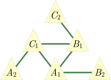
To illustrate the notion of inflation, we consider the causal structure of Fig. 1, which is called the Triangle scenario (for obvious reasons) and which has been studied recently by a number of authors [22 (Fig. E#8), 19 (Fig. 18b), 21 (Fig. 3), 33 (Fig. 6a), 40 (Fig. 1a), 47 (Fig. 8), 32 (Fig. 1b), 25 (Fig. 4b)]. Different inflations of the Triangle scenario are depicted in Figs. 2 to 6, which will be referred to as the Web, Spiral, Capped, and Cut inflation, respectively.
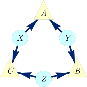
The Triangle scenario.
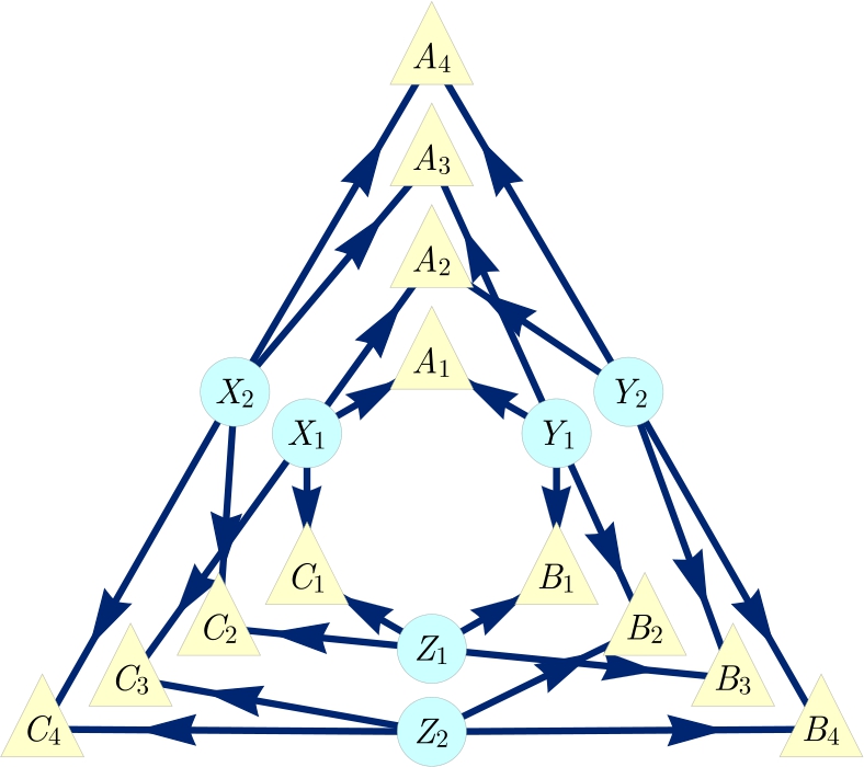
The Web inflation of the Triangle scenario where each latent node has been duplicated and each observed node has been quadrupled. The four copies of each observed node correspond to the four possible choices of parentage given the pair of copies of each latent parent of the observed node.
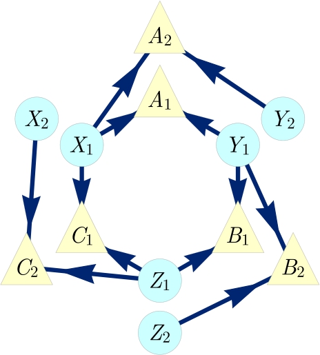
The Spiral inflation of the Triangle scenario. Notably, this causal structure is the ancestral subgraph of the set
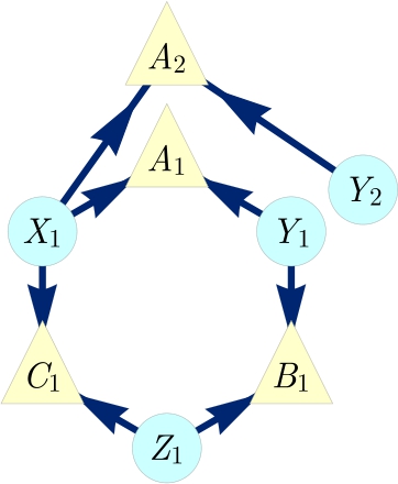
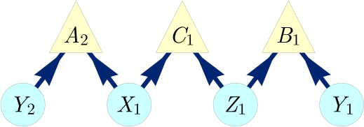
The Capped inflation of the Triangle scenario; notably also the ancestral subgraph of the set
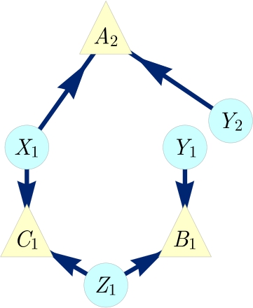
The Cut inflation of the Triangle scenario; notably also the ancestral subgraph of the set
A different depiction of the Cut inflation of Fig. 5.
We now define the function
Definition 3.
Consider causal models M and
For a given triple G,
To sum up, the inflation of a causal model is a new causal model where (i) each variable in the original causal structure may have counterparts in the inflated causal structure with ancestral subgraphs mirroring those of the originals, and (ii) the manner in which a variable depends causally on its parents in the inflated causal structure is given by the manner in which its counterpart in the original causal structure depends causally on its parents. The operation of modifying a DAG and equipping the modified version with conditional probability distributions that mirror those of the original also appears in the do calculus and twin networks of Pearl [1], and moreover bears some resemblance to the adhesivity technique used in deriving non-Shannon-type entropic inequalities (see also Appendix E).
We are now in a position to describe the key property of the inflation of a causal model, the one that makes it useful for causal inference. With notation as in Definition 3, let
This follows from the fact that the distributions on
Similarly, those sets of observed nodes in the original causal structure G which satisfy the antecedent of Eq. (7), that is, for which one can find a corresponding set in the inflated causal structure
Clearly,
For example in the Spiral inflation of the Triangle scenario depicted in Fig. 3, the set
A set of nodes in the inflated causal structure can only be injectable if it contains at most one copy of any node from the original causal structure. More strongly, it can only be injectable if its ancestral subgraph contains at most one copy of any observed or latent node from the original causal structure. Thus, in Fig. 3,
We can now express Eq. (7) in the language of injectable sets,
In the example of Fig. 3, injectability of the sets
3.2 Witnessing incompatibility
Finally, we can explain why inflation is relevant for deciding whether a distribution is compatible with a causal structure. For a distribution
The same considerations apply for any family of distributions such that each set of variables in the family corresponds to an injectable set (i. e., when the family of distributions is associated with an incomplete collection of injectable sets.) Formally,
Lemma 4.
Let the causal structure
We have thereby related a question about compatibility with the original causal structure to one about compatibility with the inflated causal structure. If one can show that the new compatibility question on
Example 1 (Incompatibility of perfect three-way correlation with the Triangle scenario).
Consider the following causal inference problem. We are given a joint distribution of three binary variables,
and we would like to determine whether it is compatible with the Triangle scenario (Fig. 1). The notation
Since there are no conditional independence relations among the observed variables in the Triangle scenario, there is no opportunity for ruling out the distribution on the grounds that it fails to satisfy the required conditional independences.
To solve the causal inference problem, we consider the Cut inflation (Fig. 5). The injectable sets include
We will show that the distribution of Eq. (11) is not compatible with the Triangle scenario by demonstrating that the contrary assumption of compatibility implies a contradiction. If the distribution of Eq. (11) were compatible with the Triangle scenario, then so too would its pair of marginals on
By Lemma 4, this compatibility assumption would entail that the marginals
are compatible with the Cut inflation of the Triangle scenario. We now show that the latter compatibility cannot hold, thereby obtaining our contradiction. It suffices to note that (i) the only joint distribution that exhibits perfect correlation between
We have therefore certified that the distribution
Example 2 (Incompatibility of the W-type distribution with the Triangle scenario).
Consider another causal inference problem on the Triangle scenario, namely, that of determining whether the distribution
is compatible with it. We call this the W-type distribution.[10] To settle this compatibility question, we consider the Spiral inflation of the Triangle scenario (Fig. 3). The injectable sets in this case include
Therefore, we turn our attention to determining whether the marginals of the W-type distribution on the images of these injectable sets are compatible with the Triangle scenario. These marginals are:
The Spiral inflation is such that
Finally, Eq. (20) together with Eq. (21) entails
This, however, contradicts Eq. (17). Consequently, the family of marginals described in Eqs. (17–19) is not compatible with the causal structure of Fig. 3. By Lemma 4, this implies that the family of marginals described in Eqs. (14–16)—and therefore the W-type distribution of which they are marginals—is not compatible with the Triangle scenario.
To our knowledge, this is a new result. In fact, the incompatibility of the W-type distribution with the Triangle scenario cannot be derived via any of the existing causal inference techniques. In particular:
Checking conditional independence relations is not relevant here, as there are no conditional independence relations between any observed variables in the Triangle scenario.
Moreover, no entropic inequality can witness the W-type distribution as unrealizable. Weilenmann and Colbeck [26] have constructed an inner approximation to the entropic cone of the Triangle causal structure, and the entropies of the W-distribution form a point in this cone. In other words, a distribution with the same entropic profile as the W-type distribution can arise from the Triangle scenario.
The newly-developed method of covariance matrix causal inference due to Kela et al. [27], which gives tighter constraints than entropic inequalities for the Triangle scenario, also cannot detect the incompatibility.
We have arrived at our incompatibility verdict by combining inflation with reasoning reminiscent of Hardy’s version of Bell’s theorem [49], [50]. Sec. 4.4 will present a generalization of this kind of argument and its applications to causal inference.
Example 3 (Incompatibility of PR-box correlations with the Bell scenario).
Bell’s theorem [17], [18], [20], [51] concerns the question of whether the distribution obtained in an experiment involving a pair of systems that are measured at space-like separation is compatible with a causal structure of the form of Fig. 7. Here, the observed variables are
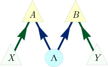
The Bell scenario causal structure. The local outcomes, A and B, of a pair of measurements are assumed to each be a function of some latent common cause and their independent local experimental settings, X and Y.
We consider the distribution
This conditional distribution was discovered by Tsirelson [54] and later independently by Popescu and Rohrlich [55], [56]. It has become known in the field of quantum foundations as the PR-box after the latter authors.[12]
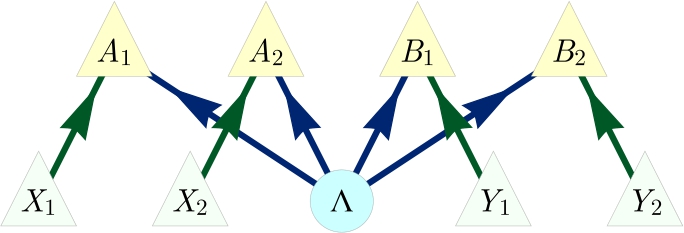
An inflation of the Bell scenario causal structure, where both local settings and outcome variables have been duplicated.
The Bell scenario implies nontrivial conditional independences[13] among the observed variables, namely,
We begin by noting that
Because
On the other hand, from Eq. (26) together with the definition of PR-box, Eq. (23), we conclude that
Combining this with Eq. (27), we obtain
No values of
The structure of this argument parallels that of standard proofs of the incompatibility of the PR-box with the Bell scenario. Standard proofs focus on a set of variables
Appendix G shows that the inflation of the Bell scenario depicted in Fig. 8 is sufficient to witness the incompatibility of any distribution that is incompatible with the Bell scenario.
3.3 Deriving causal compatibility inequalities
The inflation technique can be used not only to witness the incompatibility of a given distribution with a given causal structure, but also to derive necessary conditions that a distribution must satisfy to be compatible with the given causal structure. These conditions can always be expressed as inequalities, and we will refer to them as causal compatibility inequalities.[14] Formally, we have:
Definition 5.
Let G be a causal structure and let
While violation of a causal compatibility inequality witnesses the incompatibility with the causal structure, satisfaction of the inequality does not guarantee compatibility. This is the sense in which it merely provides a necessary condition for compatibility.
The inflation technique is useful for deriving causal compatibility inequalities because of the following consequence of Lemma 4:
Corollary 6.
Suppose that
Proof.
Suppose that the family
We now present some simple examples of causal compatibility inequalities for the Triangle scenario that one can derive from the inflation technique via Corollary 6. Some terminology and notation will facilitate their description. We refer to a pair of nodes which do not share any common ancestor as being ancestrally independent. This is equivalent to being d-separated by the empty set [1], [2], [3], [4]. Given that the conventional notation for X and Y being d-separated by Z in a DAG is
Ancestral independence is closed under union; that is,
Example 4 (A causal compatibility inequality in terms of correlators).
As in Example 1 of the previous subsection, consider the Cut inflation of the Triangle scenario (Fig. 5), where all observed variables are binary. For technical convenience, we assume that they take values in the set {−1,+1}, rather than taking values in {0,1} as was presumed in the last subsection.
The injectable sets that we make use of are
This is an example of a constraint on pairwise correlators that arises from the presumption that they are consistent with a joint distribution. (The problem of deriving such constraints is the marginal constraint problem, discussed in detail in Sec. 4.)
But in the Cut inflation of the Triangle scenario (Fig. 5),
Substituting this into Eq. (31), we have
This is an example of a simple but nontrivial causal compatibility inequality for the causal structure of Fig. 5. Finally, by Corollary 6, we infer that
is a causal compatibility inequality for the Triangle scenario. This inequality expresses the fact that as long as A and B are not completely biased, there is a tradeoff between the strength of
Given the symmetry of the Triangle scenario under permutations and sign flips of A, B and C, it is clear that the image of inequality (34) under any such symmetry is also a valid causal compatibility inequality. Together, these inequalities constitute a type of monogamy[15] of correlations in the Triangle scenario with binary variables: if any two observed variables with unbiased marginals are perfectly correlated, then they are both independent of the third.
Moreover, since inequality (31) is valid even for continuous variables with values in the interval [−1,+1], it follows that the polynomial inequality (34) is valid in this case as well.
Note that inequality (31) serves as a robust witness certifying the incompatibility of 3-way perfect correlation (described in Eq. (11)) with the Triangle scenario. Inequality (31) is robust in the sense that it demonstrates the incompatibility of distributions close to 3-way perfect correlation.
One might be curious as to how close to perfect correlation one can get while still being compatible with the Triangle scenario. To partially answer this question, we used Eq. (31) to rule out many distributions close to perfect correlation and we also pursued explicit model-construction to rule in various distributions sufficiently far from perfect correlation. Explicitly, we found that distributions of the form
where
The presence of this gap between our inner and outer constructions could reflect either the inadequacy of our limited model constructions or the inadequacy of relatively small inflations of the Triangle causal structure to generate suitably sensitive inequalities. We defer closing the gap to future work.[16]
Example 5 (A causal compatibility inequality in terms of entropic quantities).
One way to derive constraints that are independent of the cardinality of the observed variables is to express these in terms of the mutual information between observed variables rather than in terms of correlators. The inflation technique can also be applied to achieve this. To see how this works in the case of the Triangle scenario, consider again the Cut inflation (Fig. 5).
One can follow the same logic as in the preceding example, but starting from a different constraint on marginals. For any distribution on three variables
where
Substituting the latter equality into Eq. (36), we have
This is another example of a nontrivial causal compatibility inequality for the causal structure of Fig. 5. By Corollary 6, it follows that
is also a causal compatibility inequality for the Triangle scenario. This inequality was originally derived in [21]. Our rederivation in terms of inflation coincides with the proof found by Henson et al. [22].
Standard algorithms already exist for deriving entropic casual compatibility inequalities given a causal structure [25], [33], [35]. We do not expect the methodology of causal inflation to offer any computation advantage in the task of deriving entropic inequalities. The advantage of the inflation approach is that it provides a narrative for explaining an entropic inequality without reference to unobserved variables. As elaborated in Sec. 5.4, this consequently has applications to quantum information theory. A further advantage is the potential of the inflation approach to give rise to non-Shannon type inequalities, starting from Shannon type inequalities; see Appendix E for further discussion.
Example 6 (A causal compatibility inequality in terms of joint distributions).
Consider the Spiral inflation of the Triangle scenario (Fig. 3) with the injectable sets
We begin by noting that the following is a constraint that holds for any joint distribution of
To prove this claim, it suffices to check that the inequality holds for each of the
Next, we note that certain sets of variables have no common ancestors with other sets of variables in the inflated causal structure, which implies the marginal independence of these sets. Such independences are expressed in the language of joint distributions as factorizations,
Substituting these factorizations into Eq. (40), we obtain the polynomial inequality
This, therefore, is a causal compatibility inequality for the inflated causal structure. Finally, by Corollary 6, we infer that
is a causal compatibility inequality for the Triangle scenario.
What is distinctive about this inequality is that—through the presence of the term
Of the known techniques for witnessing the incompatibility of a distribution with a causal structure or deriving necessary conditions for compatibility, the most straightforward one is to consider the constraints implied by ancestral independences among the observed variables of the causal structure. The constraints derived in the last two sections have all made use of this basic technique, but at the level of the inflated causal structure rather than the original causal structure. The constraints that one thereby infers for the original causal structure reflect facts about it that cannot be expressed in terms of ancestral independences among its observed variables. The inflation technique exposes these facts in the ancestral independences among observed variables of the inflated causal structure.
In the rest of this article, we shall continue to rely only on the ancestral independences among observed variables within the inflated causal structure to derive examples of compatibility constraints on the original causal structure. Nonetheless, it seems plausible that the inflation technique can also amplify the power of other techniques that do not merely consider ancestral independences among the observed variables. We consider some prospects in Sec. 5.
4 Systematically witnessing incompatibility and deriving inequalities
This section considers the problem of how to generalize the above examples of causal inference via the inflation technique to a systematic procedure. We start by introducing the crucial concept of an expressible set, which figures implicitly in our earlier examples. By reformulating Example 1, we sketch our general method and explain why solving a marginal problem is an essential subroutine of our method. Subsequently, Sec. 4.1 explains how to systematically identify, for a given inflated causal structure, all of the sets that are expressible by virtue of ancestral independences. Sec. 4.2 describes how to solve any sort of marginal problem. This may involve determining all the facets of the marginal polytope, which is computationally costly (Appendix A). It is therefore useful to also consider relaxations of the marginal problem that are more tractable by deriving valid linear inequalities which may or may not bound the marginal polytope tightly. We describe one such approach based on possibilistic Hardy-type paradoxes and the hypergraph transversal problem in Sec. 4.4.
As far as causal compatibility inequalities are concerned, we limit ourselves to those expressed in terms of probabilities,[17] as these are generally the most powerful. However, essentially the same techniques can be used to derive inequalities expressed in terms of entropies [35], as demonstrated in Example 5.
In the examples from the previous section, the initial inequality—a constraint upon marginals that is independent of the causal structure—involves sets of observed variables that are not all injectable sets. However, the Markov conditions on the inflated causal structures nevertheless allowed us to express the distribution on these sets in terms of the known distributions on the injectable sets. For instance, in Example 4, the set
Definition 7.
Consider an inflation
For
If
An expressible set is maximal if it is not a proper subset of another expressible set.
Expressible sets are important since in an inflated model, the distribution of the variables making up an expressible set can be computed explicitly from the known distributions on the injectable sets, by repeatedly using the conditional independences implied by d-separation and taking marginals. Appendix D.1 provides a good example.
With the exception of Appendix D, in the remainder of this article we will limit ourselves to working with expressible sets of a particularly simple kind and leave the investigation of more general expressible sets to future work.
Definition 8.
A set of nodes
An ai-expressible set is maximal if it is not a proper subset of another ai-expressible set.
Because ancestral independence in
for any distribution compatible with
As a build-up to our exposition of a systematic application of the inflation technique, we now revisit Example 1. As before, to demonstrate the incompatibility of the distribution of Eq. (11) with the Triangle scenario, we assume compatibility and derive a contradiction. Given the distribution of Eq. (11), Lemma 4 implies that the marginal distributions on the injectable sets of the Cut inflation of the Triangle scenario are
and
From the fact that
But there is no three-variable distribution
Generalizing to an arbitrary causal structure, therefore, the procedure is as follows:
Based on the inflation under consideration, identify the ai-expressible sets and how they each partition into ancestrally independent injectable sets.
From the given distribution on the original causal structure, infer the family of distributions on the ai-expressible sets of the inflated causal structure as follows: the distribution on any injectable set is equal to the corresponding distribution on its image in the original causal structure; the distribution on any ai-expressible set is the product of the distributions on the injectable sets into which it is partitioned.
Determine whether the family of distributions obtained in step 2 are the marginals of a single joint distribution. If not, then the original distribution is incompatible with the original causal structure.
In summary, we have used the contrapositive of Lemma 4 in order to show:
Theorem 9.
Let
The ai-expressible sets play a crucial role in linking the original causal structure with the inflated causal structure. They are precisely those sets of variables whose joint distributions in the inflation model are fully specified by the causal model on the original causal structure, as they can be computed using Eq. (45) and Lemma 4. So we begin with the problem of identifying the ai-expressible sets systematically.
4.1 Identifying the AI-expressible sets
To identify the ai-expressible sets of an inflated causal structure
To enumerate the injectable sets, it is therefore useful to encode certain features of the inflated causal structure in an undirected graph which we call the injection graph. The nodes of the injection graph are the observed nodes of the inflated causal structure, and a pair of nodes
Given a list of the injectable sets, the ai-expressible sets can be read off from the ai-expressability graph. The nodes of the ai-expressibility graph are taken to be the injectable sets in
The injection graph corresponding to the Spiral inflation of the Triangle scenario (Fig. 3), wherein the cliques are the injectable sets.
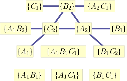
The ai-expressibility graph corresponding to the Spiral inflation of the Triangle scenario (Fig. 3), wherein two injectable sets are adjacent iff they are ancestrally independent. A set of nodes is ai-expressible iff it arises as a union of sets that form a clique in this graph.
From Figs. 9 and 10, we easily infer the injectable sets and the maximal ai-expressible sets, as well as the partition of the maximal ai-expressible sets into ancestrally independent subsets. For the Spiral example, this results in:
Having identified the ai-expressible sets and how they partition into injectable sets, we now infer the factorization relations implied by ancestral independences, which is Eq. (41) in the Spiral example. Next, we discuss the other ingredient of our systematic procedure: the marginal problem.
4.2 The marginal problem and its solution
The third step in our procedure is determining whether the given distributions on ai-expressible sets can arise as marginals of one joint distribution on all observed nodes of the inflated causal structure. In general, the problem of determining whether a given family of distributions can arise as marginals of some joint distribution is known as the marginal problem.[19] In order to derive causal compatibility inequalities, one must solve the closely related problem of determining necessary and sufficient constraints that a family of marginal distributions must satisfy in order for the marginal problem to have a solution. For better clarity, we distinguish these two variants of the marginal problem as the marginal satisfiability problem and the marginal constraint problem. The generic marginal problem will be used as an umbrella term referring to both types.
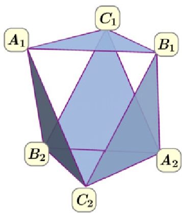
The simplicial complex of ai-expressible sets for the Spiral inflation of the Triangle scenario (Fig. 3). The 5 facets correspond to the maximal ai-expressible sets, namely
To specify either sort of marginal problem, one must specify the full set of variables to be considered, denoted
In order for
The set of all valid (positive, normalized) distributions
The map
To express this more concretely, we write the marginal satisfiability problem in the form of a generic linear program.
Let the joint distribution vector
In this notation, the marginal satisfiability problem consists of determining whether, for a given vector
where the component-wise inequality
In the example of Fig. 11 with binary variables,
Since linear programming is quite easy, probing specific distributions for compatibility for a given inflated causal structure is computationally inexpensive. For instance, using the Web inflation of the Triangle scenario (Fig. 2), which contains a large number of observed variables, our numerical computations have reproduced the result of [21, Theorem 2.16], that a certain distribution considered therein is incompatible with the Triangle scenario.[21]
In the case of the marginal constraint problem, the vector
In terms of Eq. (50), a valid inequality for the marginal distribution vector
Upon substituting the factorization relations of Eq. (45) and deleting copy indices, any valid inequality for the marginal problem turns into a causal compatibility inequality. This applies both to facet inequalities of the marginal polytope, and to Farkas infeasibility certificates. In the latter case, one obtains an explicit causal compatibility inequality which witnesses the given distribution as incompatible with the given causal structure. In other words, if a given distribution is witnessed as incompatible with a causal structure using the technique we have described, then with little additional numerical effort, one can also obtain a causal compatibility inequality that exhibits the incompatibility. This may have applications to problems where the facet enumeration is computationally intractable.
Summarizing, we have shown how to leverage the marginal satisfiability problem to witness causal incompatibility of particular distributions, and how to leverage the marginal constraint problem to derive causal compatibility inequalities.
4.3 A list of causal compatibility inequalities for the triangle scenario
As an example of the above method, we have considered the Triangle scenario with binary observed variables and derived all causal compatibility inequalities which follow by means of using ancestral independences in the Spiral inflation (Fig. 3). We found that there are 4884 inequalities corresponding to the facets of the relevant marginal polytope, which results in 4884 polynomial causal compatibility inequalities for the Triangle scenario.
However, most inequalities in this set have turned out to be redundant, where an inequality is considered redundant if there is no distribution that violates this inequality but none of the others. We thus have looked for a subset of inequalities that is irredundant (does not contain any redundant inequality) but nevertheless complete (defines the same set of distributions as the full set). While a finite system of linear inequalities always has a unique irredundant complete subset, this need not be the case for finite systems of polynomial inequalities; we therefore speak of “a” complete irredundant set instead of “the” complete irredundant set.
We exploited linear programming techniques to quickly identify a 1433-inequalities complete subset of our original 4884 inequalities; concretely, the copy isomorphisms of Appendix C yield an additional list of linear equations satisfied by all inflation models, and from every set of inequalities that differ by merely a linear combination of these equations we choose one representative. To further prune away redundant inequalities, we successively employed nonlinear constrained maximization on each inequality’s left-hand-side, to determine numerically if it could be violated pursuant to all the other inequalities as constraints. An inequality is found to be redundant if the solution to the constrained maximization does not exceed the inequality’s right-hand side. Such an inequality was immediately dropped from the set before testing the next candidate for redundancy.[25] This post-processing led us to identify 60 irredundant inequalities which defines the same set of satisfying distributions as the original 4884. Of the remaining 60, we recognized 8 as uninteresting positivity inequalities,
To present those inequalities in an efficient manner, we further grouped them into four symmetry classes. In Eqs. (51–54) we present one representative from each class; the multiplicity of inequalities contained in each symmetry class is marked in parentheses. The symmetry group for any causal structure with finite-cardinality observed variables is generated by those permutations of the observed variables which can be extended to automorphisms of the (original) DAG, as well as any permutation among the discrete values assigned to an individual observed variable (i. e., bijections on the sample space of that variable). In the case of the Triangle scenario with binary observed variables, the symmetry group therefore has 48 elements, comprised of the 6 permutations of the three observed variables, the three local binary-value relabellings, and all their compositions (48=6×2×2×2).
We choose to express our inequalities in terms of correlators (where the two possible values of each variables to be {−1,+1}), rather than in terms of joint probabilities, because such a presentation is more compact:
A machine-readable and closed-under-symmetries version of this list of inequalities may be found in Appendix F.
4.4 Causal compatibility inequalities via hardy-type inferences from logical tautologies
Enumerating all the facets of the marginal polytope is computationally feasible only for small examples. But our method transforms every inequality that bounds the marginal polytope into a causal compatibility inequality. We now present a general approach for deriving a special type of such inequalities very quickly.
In the literature on Bell inequalities, it has been noticed that incompatibility with the Bell causal structure can sometimes be witnessed by merely looking at which joint outcomes have zero probability and which ones have nonzero probability. In other words, instead of considering the probability of an outcome, the inconsistency of some marginal distributions can be evident from considering only the possibility or impossibility of each outcome. This insight is originally due to Hardy [49], and versions of Bell’s theorem that are based on the violation of such possibilistic constraints are known as Hardy-type paradoxes [57], [70], [71], [72], [73]; a partial classification of these can be found in [50]. The method that we describe in the second half of this section can be used to compute a complete classification of possibilistic constraints for any marginal problem.
Possibilistic constraints follow from a consideration of logical relations that can hold among deterministic assignments to the observed variables. Such logical constraints can also be leveraged to derive probabilistic constraints instead of possibilistic ones, as shown in [60], [74]. This results in a partial solution to any given (probabilistic) marginal problem. Essentially, we solve a possibilistic marginal problem [50], then upgrade the possibilistic constraints into probabilistic inequalities, resulting in a set of probabilistic inequalities whose satisfaction is a necessary but insufficient condition for satisfying the corresponding probabilistic marginal problem. We now demonstrate how to systematically derive all inequalities of this type.
We have already provided a simple example of a Hardy-type argument in Example 2, in the logic used to demonstrate that the family of distributions of Eqs. (17–19) cannot arise as the marginals of a single joint distribution. For our present purposes, it is useful to recast that argument into a new but manifestly equivalent form. First, for the family of distributions in question, we have
From the last constraint one infers that at least one of
However, the Spiral inflation (Fig. 3) is such that
We are here interested in recasting the argument in a manner amenable to systematic generalization. This is done as follows. We work in a marginal scenario where the contexts are
is a logical tautology for binary variables. It can be understood as a constraint on marginal deterministic assignments, which can be thought of as a logical counterpart of a linear inequality bounding the marginal polytope. The second and final step of the argument notes that the given marginal distributions are such that the antecedent is always true, while the consequent is sometimes false.
To see how to translate this into a constraint on marginal distributions, we rewrite Eq. (57) in its contrapositive form,

Next, we note that if a logical tautology can be expressed as
then by applying the union bound—which asserts that the probability of at least one of a set of events occurring is no greater than the sum of the probabilities of each event occurring—one obtains
Applying this to Eq. (58) in particular yields

which is a constraint on the marginal distributions.
This inequality allows one to demonstrate the incompatibility of the family of distributions of Eqs. (17–19) with the Spiral inflation just as easily as one can with the tautology of Eq. (57). The fact that
As another example, consider the marginal problem where the variables are A, B and C, with each being binary, and the contexts are the pairs

Applying the union bound, one obtains a constraint on marginal distributions,[28]

In this section, we seek to determine, for any marginal scenario, the set of all inequalities that can be derived in this manner. We do so by enumerating the full set of tautologies of the form of Eqs. (57, 62). This boils down to solving the possibilistic version of the marginal constraint problem.
We now describe the general procedure. As before, we express a constraint on marginal deterministic assignments as a logical implication, having a valuation (assignment of outcomes) on one context as the antecedent and a disjunction over valuations on contexts as the consequent. In the following, we explain how to generate all such implications which are tight in the sense that the consequent is minimal, i. e., involves as few terms as possible in the disjunction.
First, we fix the antecedent by choosing some context and a joint valuation of its variables. In order to generate all constraints on marginal deterministic assignments, one will have to perform this procedure for every context as the antecedent and every choice of valuation thereon. For the sake of concreteness, we take the above Spiral inflation example with  as the antecedent. Each logical implication we consider is required to have the property that any variable that appears in both the antecedent and the consequent must be given the same value in both.
To formally determine all valid consequents, it is useful to introduce two hypergraphs associated to the problem. Recall the definition of the incidence matrix of a hypergraph: if vertex i is contained in edge j of the hypergraph, the component in the ith row and jth column of the matrix is 1; otherwise it is 0.
The first hypergraph we consider is the one whose incidence matrix is the marginal description matrix  contains the vertex
  . In our example following Fig. 11, this initial hypergraph has
The second hypergraph is a subhypergraph of the first one. We delete from the first hypergraph all vertices and hyperedges which contradict the outcomes supposed by the antecedent. In our example, because the vertex  contradicts the antecedent
  , we delete it. We also delete the vertex corresponding to the antecedent itself. In our example, this second hypergraph has
All valid (minimal) consequents are (minimal) transversals of this latter hypergraph. A transversal is a set of vertices which has the property that it intersects every hyperedge in at least one vertex. In order to get implications which are as tight as possible, it is sufficient to enumerate only the minimal transversals. Doing so is a well-studied problem in computer science with various natural reformulations and for which manifold algorithms have been developed [75].
In our example, it is not hard to check that the consequent of

is such a minimal transversal: every assignment of values to all variables which extends the assignment on the left-hand side satisfies at least one of the terms on the right, but this ceases to hold as soon as one removes any one term on the right.
We convert these implications into inequalities in the usual way via the union bound (i. e., replacing “⇒” by “≤” at the level of probabilities and the disjunction by summation). Thus Eq. (63) translates into the constraint on marginal distributions

This inequality constitutes a strengthening of Eq. (61) that we had used as Eq. (40) as the starting point for deriving a causal compatibility inequality for the Triangle scenario, Eq. (43).
Inequalities that one derives from hypergraph transversals are generally weaker than those that result from a complete solution of the marginal problem. Nevertheless, many Bell inequalities are of this form, the CHSH inequality among them [74]. So it seems that this method is still sufficiently powerful to generate plenty of interesting inequalities. At the same time, the method is significantly less computationally costly than the full-fledged facet enumeration, even if one does it for every possible antecedent. Interestingly, all of the irredundant polynomial inequalities represented in Eqs. (51–54) are found to be derivable by means of hypergraph transversals.
In conclusion, facet enumeration is the preferred method for deriving inequalities for the marginal problem when it is computationally tractable. When it is not, enumerating hypergraph transversals presents a good alternative.
5 Further prospects for the inflation technique
Lemma 4 and Corollary 6 state that any causal inference technique on an inflated causal structure
5.1 Appealing to d-separation relations in the inflated causal structure beyond ancestral independance
In Sec. 4, we considered the inflation technique using sets of observed variables on the inflated causal structure that were ai-expressible, that is, that can be written as a union of injectable sets that are ancestrally independent. However, it is standard practice when deriving causal compatibility conditions for a causal structure to make use not just of ancestral independences, but of arbitrary d-separation relations among variables, and for this reason we had also introduced the notion of expressible set in Sec. 4. We now comment on the utility of general expressible sets for the inflation technique.
In a given causal structure, if sets of variables
For
The answer is that it can. Consider an inflation
It follows that if one includes expressible sets such as
In Appendix D, we provide a concrete example of how a d-separation relation distinct from ancestral independence can be useful both for the problem of witnessing the incompatibility of a specific distribution with a causal structure and for the problem of deriving causal compatibility inequalities.
Per Definition 7, the notion of expressibility is recursive: The set
5.2 Imposing symmetries from copy-index-equivalent subgraphs of the inflated causal structure
By the definition of an inflation model (Definition 3), if two variables in the inflated causal structure
The ancestral subgraphs of
For example, consider the pair of contexts
We can similarly conclude that in the inflation model these marginal distributions satisfy
These constraints entail that
Parameters such as
The general problem of finding pairs of contexts in the inflated causal structure for which relations of copy-index-equivalence imply equality of the marginal distributions, and the conditions under which such equalities may yield tighter inequalities, are discussed in more detail in Appendix C.
5.3 Incorporating nonlinear constraints
In deriving causal compatibility inequalities and in witnessing causal incompatibility of a specific distribution, we restricted ourselves to starting from the marginal problem where the contexts are the (ai-)expressible sets, and wherein one imposes only linear constraints derived from the marginal problem. In this approach, facts about the causal structure only get incorporated in the construction of the marginal distribution on each expressible set, and the quantifier elimination step of the computational algorithm is linear. However, one can also incorporate facts about the causal structure as constraints on the quantifier elimination problem at the cost making the quantifier elimination problem nonlinear.
Take the Spiral inflation of the Triangle scenario as an example. There is an ancestral independence therein that we did not use in our previous application of the inflation technique, namely,
Recall that in the marginal problem, one seeks to eliminate the unknowns
together with linear inequalities expressing the nonnegativity of the
One can incorporate any d-separation relation in the inflated causal structure in this manner. For instance, if
However, because
On the one hand, many modern computer algebra systems do have functions capable of tackling nonlinear quantifier elimination symbolically.[30] Currently, however, it is generally not practical to perform nonlinear quantifier elimination on large polynomial systems with many unknowns to be eliminated. It may help to exploit results on the concrete algebraic-geometric structure of these particular systems [11].
If one is seeking merely to assess the compatibility of a given distribution with the causal structure, then one can avoid the quantifier elimination problem and simply try and solve an existence problem: after substituting the values that the given distribution prescribes for the outcomes on ai-expressible sets into the polynomial system in terms of the unknown global joint probabilities, one must only determine whether that system has a solution. Most computer algebra systems can resolve such satisfiability questions quite easily.[31]
It is also possible to use a mixed strategy of linear and nonlinear quantifier elimination, such as Chaves [9] advocates. The explicit results of [9] are directly causal implications of the original causal structure, achieved by applying a mixed quantifier elimination strategy. Perhaps further causal compatibility inequalities will be derivable by applying such a mixed quantifier elimination strategy to the inflated causal structure.
5.4 Implications of the inflation technique for quantum physics and generalized probabilistic theories
This specialized subsection is intended specifically for those readers already somewhat proficient with fundamental concepts in quantum theory. Non-physicists may wish to skip ahead to the conclusions (Sec. 6).
Recent work has sought to explore quantum generalizations of the notion of a causal model, termed quantum causal models [22], [23], [39], [40], [41], [42], [43]. We here use the quantum generalization that is implied by the approach of [22] and closely related to the one of [23].
The causal structures are still represented by DAGs, supplemented with a distinction between observed and latent nodes. However, the latent nodes are now associated with families of quantum channels and the observed nodes are now associated with families of quantum measurements. Observed nodes are still labelled by random variables, which represent the outcome of the associated measurement. One also makes a distinction between edges in the DAG that carry classical information and edges that carry quantum information.[32] An observed node can have incoming edges of either type: those that come from other observed nodes carry classical information, while those that come from latent nodes carry quantum information. Each quantum measurement in the set that is associated to an observed node acts on the collection of quantum systems received by this node (i. e., on the tensor product of the Hilbert spaces associated to the incoming edges). The classical variables that are received by the node act collectively as a control variable, determining which measurement in the set is implemented. Finally, the random variable that is associated to the node encodes the outcome of the measurement. All of the outgoing edges of an observed node are classical and simply broadcast the outcome of the measurement to the children nodes. A latent node can also have incoming edges that carry classical variables as well as incoming edges that carry quantum systems. Each quantum channel in the set that is associated to a latent node takes the collection of quantum systems associated to the incoming edges as its quantum input and the collection of quantum systems associated to the outgoing edges as its quantum output (the input and output spaces need not have the same dimension). The classical variables that are received by the node act collectively as a control variable, determining which channel in the set is implemented.
A quantum causal model is still ultimately in the service of explaining joint distributions of observed classical variables. The joint distribution of these variables is the only experimental data with which one can confront a given quantum causal model. The basic problem of causal inference for quantum causal models, therefore, concerns the compatibility of a joint distribution of observed classical variables with a given causal structure, where the model supplementing the causal structure is allowed to be quantum, in the sense defined above. If this happens, we say that the distribution is quantumly compatible with the causal structure.
One motivation for studying quantum causal models is that they offer a new perspective on an old problem in the field of quantum foundations: that of establishing precisely which of the principles of classical physics must be abandoned in quantum physics. It was noticed by Fritz [21] and Wood and Spekkens [19] that Bell’s theorem [51] states that there are distributions on observed nodes of the Bell causal structure that are quantumly compatible but not classically compatible with it. Moreover, it was shown in [19] that these distributions cannot be explained by any causal structure while complying with the additional principle that conditional independences should not be fine-tuned, i. e., while demanding that any observed conditional independence should be accounted for by a d-separation relation in the DAG. These results suggest that quantum theory is perhaps best understood as revising our notions of the nature of unobserved entities, and of how one represents causal dependences thereon and incomplete knowledge thereof, while nonetheless preserving the spirit of causality and the principle of no fine-tuning [39], [84], [85].
Another motivation for studying quantum causal models is a practical one. Violations of Bell inequalities have been shown to constitute resources for information processing [86], [87], [88]. Hence it seems plausible that if one can find more causal structures for which there exist distributions that are quantumly compatible but not classically so, then this quantum-classical separation may also find applications to information processing. For example, it has been shown that in addition to the Bell scenario, such a quantum-classical separation also exists in the bilocality scenario [47] and the Triangle scenario [21], and it is likely that many more causal structures with this property will be found, some with potential applicability to information processing.
So for both foundational and practical reasons, there is good reason to find examples of causal structures that exhibit a quantum-classical separation. However, this is by no means an easy task. The set of distributions that are quantumly compatible with a given causal structure is quite hard to separate from the set of distributions that are classically compatible [21], [22]. For example, both the classical and quantum sets respect the conditional independence relations among observed nodes that are implied by the d-separation relations of the DAG [22], and entropic inequalities are only of very limited use [21], [89]. We hope that the inflation technique will provide better tools for finding such separations.
In addition to quantum generalizations of causal models, one can define generalizations for other operational theories that are neither classical nor quantum [22], [23]. Such generalizations are formalized using the framework of generalized probabilistic theories (GPTs) [90], [91], which is sufficiently general to describe any operational theory that makes statistical predictions about the outcomes of experiments and passes some basic sanity checks. Some constraints on compatibility can be proven to be theory-independent in that they apply not only to classical and quantum causal models, but to any kind of generalized probabilistic causal model [22]. For example, the classically-valid conditional independence relations that hold among observed variables in a causal structure are all also valid in the GPT framework. Another example is the entropic monogamy inequality Eq. (39), which was proven in [22] to be GPT valid as well. These kinds of constraints are of interest because they clarify what any conceivable theory of physics must satisfy on a given causal structure.
The essential element in deriving such constraints is to only make reference to the observed nodes, as done in [22]. In fact, we now understand the argument of [22] to be an instance of the inflation technique. Nonetheless, we have seen that the inflation technique often yields inequalities that hold for the classical notion of compatibility, while having quantum and GPT violations, such as the Bell inequalities of Example 3 of Sec. 3.2 and Appendix G. In fact, inflation can be used to derive inequalities with quantum violations for the Triangle scenario as well [92].
So what distinguishes applications of the inflation technique that yield inequalities for GPT compatibility from those that yield inequalities for classical compatibility? The distinction rests on a structural feature of the inflation:
Definition 10.
In
The Web and Spiral inflations of the Triangle scenario, depicted in Fig. 2 and Fig. 3 respectively, contain one or more inflationary fan-outs, as does the inflation of the Bell causal structure that is depicted in Fig. 8. On the other hand, the simplest inflation of the Triangle scenario that we consider in this article, the Cut inflation depicted in Fig. 5, does not contain any inflationary fan-outs.
Our main observation is that if one uses an inflation without an inflationary fan-out, then the resulting inequalities derived by the inflation technique will all be GPT valid. In other words, one can only hope to detect a GPT-classical separation if one uses an inflation that has at least one inflationary fan-out. We now explain the intuition for why this is the case. In the classical causal model obtained by inflation, the copy-index-equivalent children of an inflationary fan-out causally depend on their parent node in precisely the same way as their counterparts in the original causal structure do. For example, this dependence may be such that these two children are exact copies of the inflationary fan-out node. So when one tries to write down a GPT version of our notion of inflation, one quickly runs into trouble: in quantum theory, the no-broadcasting theorem shows that such duplication is impossible in a strong sense [93], and an analogous theorem holds for GPTs [94]. This is why in the presence of an inflationary fan-out, one cannot expect our inequalities to hold in the quantum or GPT case, which is consistent with the fact that they often do have quantum and GPT violations.
On the other hand, for any inflation that does not contain an inflationary fan-out, the notion of an inflation model generalizes to all GPTs; we sketch how this works for the case of quantum theory. By the definition of inflation, any node in
All of these assertions about inflations that do not contain any inflationary fan-outs apply not only to quantum causal models, but to GPT causal models as well, using the definition of the latter provided in [22].
In the remainder of this section, we discuss the relation between the quantum and the GPT case. Since quantum theory is a particular generalized probabilistic theory, quantum compatibility trivially implies GPT compatibility. Through the work of Tsirelson [54] and Popescu and Rohrlich [55], it is known that the converse is not true: the Bell scenario manifests a GPT-quantum separation. The identification of distributions witnessing this difference, and the derivation of quantum causal compatibility inequalities with GPT violations, has been a focus of much foundational research in recent years. Traditionally, the foundational question has always been: why does quantum theory predict correlations that are stronger than one would expect classically? But now there is a new question being asked: why does quantum theory only allow correlations that are weaker than those predicted by other GPTs? There has been some interesting progress in identifying physical principles that can pick out the precise correlations that are exhibited by quantum theory [95], [96], [97], [98], [99], [100], [101], [102], [103]. Further opportunities for identifying such principles would be useful. This motivates the problem of classifying causal structures into those which have a quantum-classical separation, those which have a GPT-quantum separation and those which have both. Similarly, one can try to classify causal compatibility inequalities into those which are GPT-valid, those which are GPT-violable but quantumly valid, and those which are quantum-violable but classically valid.
The problem of deriving inequalities that are GPT-violable but quantumly valid is particularly interesting. Chaves et al. [40] have derived some entropic inequalities that can do so. At present, however, we do not see a way of applying the inflation technique to this problem.
6 Conclusions
We have described the inflation technique for causal inference in the presence of latent variables.
We have shown how many existing techniques for witnessing incompatibility and for deriving causal compatibility inequalities can be enhanced by the inflation technique, independently of whether these pertain to entropic quantities, correlators or probabilities. The computational difficulty of achieving this enhancement depends on the seed technique. We summarize the computational difficulty of the approaches that we have considered in Table 1. A similar table could be drawn for the satisfiability problem, with relative difficulties preserved, but where none of the variants of the problem are computationally hard.
A comparison of different approaches for deriving constraints on compatibility at the level of the inflated causal structure, which then translate into constraints on compatibility at the level of the original causal structure.
| Type of constraints imposed on the joint distribution over all observed variables in the inflated graph | General problem | → | Standard algorithm(s) | Difficulty |
| Marginal compatibility, i. e., the joint distribution should recover all expressible (or ai-expressible) distributions as marginals (Sec. 5.1) | Facet enumeration of marginal polytope (Sec. 4.2) | → | see Appendix A | Hard |
| Finding possibilistic constraints by identifying hypergraph transversals (Sec. 4.4) | → | see Eiter et al. [75] | Very easy | |
| Whenever two equivalent-up-to-copy-indices sets of observed variables have ancestral subgraphs which are also equivalent-up-to-copy-indices, then the marginals over said variables must coincide (Sec. 5.2) | Marginal problem with additional equality constraints, therefore linear quantifier elimination (Appendix C) | → | Fourier-Motzkin elimination [77], [78], [79], [80], [81], Equality set projection [82], [83] | Hard |
| The joint distribution should satisfy all conditional independence relations implied by d-separation conditions on the observed variables (Sec. 5.3) | Real (nonlinear) quantifier elimination | → | Cylindrical algebraic decomposition [9] | Very hard |
Especially in Sec. 4, we have focused on one particular seed technique: the existence of a joint distribution on all observed nodes together with ancestral independences. We have shown how a complete or partial solution of the marginal problem for the ai-expressible sets of the inflated causal structure can be leveraged to obtain criteria for causal compatibility, both at the level of witnessing particular distributions as incompatible and deriving causal compatibility inequalities. These inequalities are polynomial in the joint probabilities of the observed variables. They are capable of exhibiting the incompatibility of the W-type distribution with the Triangle scenario, while entropic techniques cannot, so that our polynomial inequalities are stronger than entropic inequalities in at least some cases (see Example 2 of Sec. 3.2). As far as we can tell, our inequalities are not related to the nonlinear causal compatibility inequalities which have been derived specifically to constrain classical networks [28], [29], [30], nor to the nonlinear inequalities which account for interventions to a given causal structure [53], [104].
We have shown that some of the causal compatibility inequalities we derive by the inflation technique are necessary conditions not only for compatibility with a classical causal model, but also for compatibility with a causal model in any generalized probabilistic theory, which includes quantum causal models as a special case. It would be enlightening to understand the general extent to which our polynomial inequalities for a given causal structure can be violated by a distribution arising in a quantum causal model. A variety of techniques exist for estimating the amount by which a Bell inequality [105], [106] is violated in quantum theory, but even finding a quantum violation of one of our polynomial inequalities for causal structures other than the Bell scenario presents a new task for which we currently lack a systematic approach. Nevertheless, we know that there exists a difference between classical and quantum also beyond Bell scenarios [21, Theorem 2.16], and we hope that our polynomial inequalities will perform better in probing this separation than entropic inequalities do [22], [40].
We have shown that the inflation technique can also be used to derive causal compatibility inequalities that hold for arbitrary generalized probabilistic theories, a significant generalization of the results of [22]. Such inequalities are also very significant insofar as they constitute a restriction on the sorts of statistical correlations that could arise in a given causal scenario even if quantum theory is superseded by some alternative physical theory. As long as the successor theory falls within the framework of generalized probabilistic theories, the restriction will hold.
Finally, an interesting question is whether it might be possible to modify our methods somehow to derive causal compatibility inequalities that hold for quantum theory and are violated by some GPT. Since the initial drafting of this manuscript, such a modification has been identified [107].
A single causal structure has an unlimited number of potential inflations. Selecting a good inflation from which strong polynomial inequalities can be derived is an interesting challenge. To this end, it would be desirable to understand how particular features of the original causal structure are exposed when different nodes in the causal structure are duplicated. By isolating which features are exposed in each inflation, we could conceivably quantify the utility for causal inference of each inflation. In so doing, we might find that inflations beyond a certain level of variable duplication need not be considered. The multiplicity beyond which further inflation is irrelevant may be related to the maximum degree of those polynomials which tightly characterize a causal scenario. Presently, however, it is not clear how to upper bound either number, though a finite upper bound on the maximum degree of the polynomials follows from the semialgebraicity of the compatible distributions, per Ref. [6].
Causal compatibility inequalities are, by definition, merely necessary conditions for compatibility. Depending on what kind of causal inference methods one uses at the level of an inflated causal structure
Significantly, since the initial drafting of this manuscript, Ref. [108] has proven that the inflation technique indeed gives necessary and sufficient conditions for causal compatibility: any incompatible distribution is witnessed as incompatible by a suitably large inflation. Ref. [108] also provides other interesting results, such as a prescription for how to generate all relevant inflations, as well as an explicit demonstration of the inflation technique as applied to Pearl’s instrumental scenario.
Funding source: John Templeton Foundation
Award Identifier / Grant number: 69609
Funding statement: This project/publication was made possible in part through the support of a grant #69609 from the John Templeton Foundation. The opinions expressed in this publication are those of the authors and do not necessarily reflect the views of the John Templeton Foundation. This research was supported in part by Perimeter Institute for Theoretical Physics. Research at Perimeter Institute is supported in part by the Government of Canada through the Department of Innovation, Science and Economic Development Canada and by the Province of Ontario through the Ministry of Economic Development, Job Creation and Trade.
Acknowledgment
E. W. would like to thank Rafael Chaves, Miguel Navascues, and T. C. Fraser for suggestions which have improved this manuscript. T. F. would like to thank Nihat Ay and Guido Montúfar for discussion and references. Part of this research was conducted while T. F. was with the Max Planck Institute for Mathematics in the Sciences.
Appendix A Algorithms for solving the marginal constraint problem
By solving the marginal constraint problem, what we mean is to determine all the facets of the marginal polytope for a given marginal scenario. Since the vertices of this polytope are precisely the deterministic assignments of values to all variables, which are easy to enumerate, solving the marginal constraint problem is an instance of a facet enumeration problem: given the vertices of a convex polytope, determine its facets. This is a well-studied problem in combinatorial optimization for which a variety of algorithms are available [109].
A generic facet enumeration problem takes a matrix
To solve the marginal problem one uses the marginal description matrix introduced in Sec. 4.2 as the input to the facet enumeration algorithm, i. e.
The oldest-known method for facet enumeration relies on linear quantifier elimination in the form of Fourier-Motzkin (FM) elimination [77], [78]. This refers to the fact that one starts with the system
Other algorithms for facet enumeration that are not based on linear quantifier elimination include the following. Lexicographic reverse search (LRS) [112] explores the entire polytope by repeatedly pivoting from one facet to an adjacent one, and is implemented in lrs. Equality Set Projection (ESP) [82], [83] is also based on pivoting from facet to facet, though its implementation is less stable.[34] These algorithms could be interesting to use in practice, since each pivoting step churns out a new facet; by contrast, Fourier-Motzkin type algorithms only generate the entire list of facets at once, after all the quantifiers have been eliminated one by one, see Ref. [113] for a recent comparative review.
It may also be possible to exploit special features of marginal polytopes in order to facilitate their facet enumeration, such as their high degree of symmetry: permuting the outcomes of each variable maps the polytope to itself, which already generates a sizeable symmetry group, and oftentimes there are additional symmetries given by permuting some of the variables. This simplifies the problem of facet enumeration [114], [115], and it may be interesting to apply dedicated software[35] to the facet enumeration problem of marginal polytopes [116], [117], [118].
Appendix B Explicit marginal description matrix of the cut inflation with binary observed variables
The three maximal ai-expressible sets of the Cut inflation (Fig. 5) are
As we noted in the main text, such conditions can be expressed in terms of a single matrix equality,
and hence the marginal description matrix
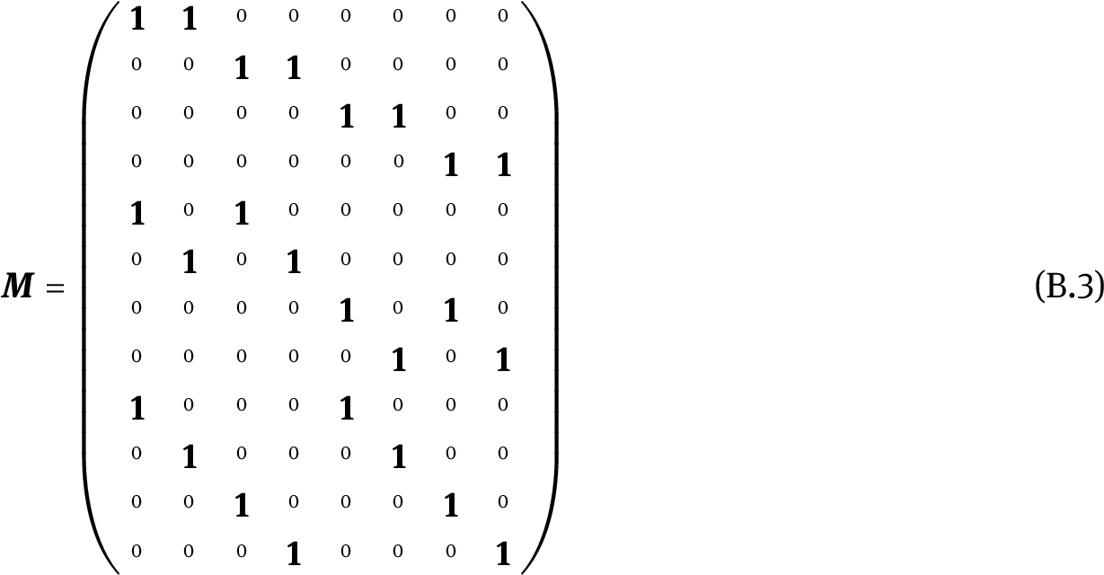
such that
Appendix C Constraints on marginal distributions from copy-index equivalence relations
In Sec. 5.2, we noted that every copy of a variable in an inflation model has the same probabilistic dependence on its parents as every other copy. It followed that for certain pairs of marginal contexts, the marginal distributions in any inflation model are necessarily equal. We now describe not only how to identify all such pairs of contexts, but also how to identify weak pairs, who’s corresponding symmetry imposition cannot help strengthen the final constraints.
Given
Furthermore, we say that a copy isomorphism
For given observed
Lemma 11.
Let
This applies in particular when
Lemma 11 is best illustrated by returning to our example from Sec. 5.2 which considered the Spiral inflation of Fig. 3 and the pair of contexts
is a copy isomorphism between
which is again a copy isomorphism. Therefore φ is indeed an inflationary isomorphism. From Lemma 11, we then conclude that any inflation model satisfies
Similarly, the map
is also easily verified to be a copy isomorphism between
so that
![Figure 12 The instrumental scenario of Pearl [31].](/document/doi/10.1515/jci-2017-0020/asset/graphic/j_jci-2017-0020_fig_012.jpg)
The instrumental scenario of Pearl [31].
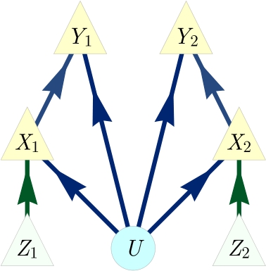
An inflation of the instrumental scenario which illustrates why coinciding ancestral subgraphs doesn’t necessarily imply coinciding marginal distributions.
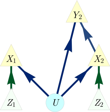
The ancestral subgraph of Fig. 13 for either
In order to avoid any possibility of confusion, we emphasize that it is not a plain copy isomorphism between the subgraphs of
One can try to make use of Lemma 11 when deriving polynomial inequalities with inflation via solving the marginal problem, by imposing the resulting equations of the form
In some cases, this lack of impact can be explained as follows. Suppose that
Suppose that some joint distribution
This argument does not apply when the inflationary isomorphism
Appendix D Using the inflation technique to certify a causal structure as “interesting”
By considering all possible d-separation relations on the observed nodes of a causal structure, one can infer the set of all conditional independence (CI) relations that must hold in any distribution compatible with it. Due to the presence of latent variables, satisfying these CI relations is generally not sufficient for compatibility. Henson, Lal and Pusey (HLP) [22] introduced the term interesting for those causal structures for which this happens, and derived a partial classification of causal structures into interesting and non-interesting ones by finding necessary criteria for a causal structure to be interesting, and they also conjectured their criteria to be sufficient. As evidence in favour of this conjecture, they enumerated all possible isomorphism classes of causal structure with up to six nodes satisfying their criteria, which resulted in only 21 equivalence classes of potentially interesting causal structures. Of those 21, they further proved that 18 were indeed interesting by writing down explicit distributions which are incompatible despite satisfying the observed CI relations. Incompatibility was certified by means of entropic inequalities.
That left three classes of causal structures as potentially interesting (Figs. 15–17). For each of these, HLP derived both: (i) the set of Shannon-type entropic inequalities that take into account the CI relations among the observed variables, and (ii) the set of Shannon-type entropic inequalities that also take into account CI relations among latent variables. Finding the second set to be larger than the first constitutes evidence that the causal structure is interesting. The evidence is not conclusive, however, because the Shannon-type inequalities that are included in the second set but not the first might be non-Shannon-type inequalities that merely follow from the CI relations among the observed variables [22].
One way to close this loophole would be to show that the novel Shannon-type inequalities imply constraints beyond some inner approximation to the genuine entropic cone corresponding to the CI relations among observed variables, perhaps along the lines of [26]. Another is to use causal compatibility inequalities beyond entropic inequalities to identify some CI-respecting but incompatible distributions. Pienaar [36] accomplished precisely this by considering the different values that an observed root variable may take. In the following, we demonstrate how the inflation technique can be used for the same purpose.
![Figure 15 Causal structure #15 in [22]. The d-separation relations are C⊥dYC{\perp _{d}}Y and A⊥dB|YA{\perp _{d}}B\hspace{0.1667em}|\hspace{0.1667em}Y.](/document/doi/10.1515/jci-2017-0020/asset/graphic/j_jci-2017-0020_fig_015.jpg)
Causal structure #15 in [22]. The d-separation relations are
![Figure 16 Causal structure #16 in [22]. The only d-separation relation is C⊥dYC{\perp _{d}}Y.](/document/doi/10.1515/jci-2017-0020/asset/graphic/j_jci-2017-0020_fig_016.jpg)
Causal structure #16 in [22]. The only d-separation relation is
![Figure 17 Causal structure #20 in [22]. The d-separation relations are C⊥dYC{\perp _{d}}Y and A⊥dY|BA{\perp _{d}}Y\hspace{0.1667em}|\hspace{0.1667em}B.](/document/doi/10.1515/jci-2017-0020/asset/graphic/j_jci-2017-0020_fig_017.jpg)
Causal structure #20 in [22]. The d-separation relations are
D.1 Certifying that Henson-Lal-Pusey’s causal structure #16 is “interesting”
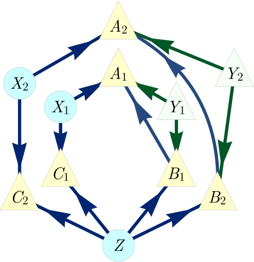
The Russian dolls inflation of Fig. 16.
Pienaar [ 36] identified a distribution which satisfies the only CI relation that must hold among the observed variables in HLP’s causal structure #16 (Fig. 16), namely,
It is useful to compute the conditional on Y,
This makes it evident that the distribution can be described as follows: if
Here, we will establish the incompatibility of Pienaar’s distribution with HLP’s causal structure #16 (reproduced in Fig. 16 here) using the inflation technique. To do so, we use the inflation depicted in Fig. 18, which we term the Russian dolls inflation. We will make use of the fact that
We begin by demonstrating how the d-separation relations in the Russian dolls inflation imply that
and the sets
It follows that the distribution
and from Eq. (D.4) and (D.3), as well as the injectability of
We are now in a position to derive a contradiction. Our derivation will begin by setting
and similarly from Eq. (D.6),
From these and Eq. (D.2), we infer
From Eq. (D.9), we have
From Eq. (D.10), we have
These three statements imply that
However, Eq. (D.12) implies that the probability of
D.2 Deriving a causal compatibility inequality for HLP’s causal structure #16
We can also turn the above argument into an inequality. Using the methods of Sec. 4.4, it is straightforward to show that the assumption of a joint distribution on
From the following four ancestral independences in the inflated causal structure,
Substituting these into Eq. (D.17), we obtain:
This is a nontrivial causal compatibility inequality for the inflated causal structure. However, in this form, it cannot be translated into one for the observed variables in the original causal structure: the sets
This is also a nontrivial causal compatibility inequality for the inflated causal structure, but now it refers exclusively to distributions on injectable sets. As such, we can directly translate it into a nontrivial causal compatibility inequality for the original causal structure, namely,
Dividing by
This inequality is strong enough to witness the incompatibility of Pienaar’s distribution Eq. (D.1) with HLP’s causal structure
D.3 Certifying that Henson-Lal-Pusey’s causal structures #15 and #20 are “interesting”
Any distribution
It follows that if one can find a distribution that exhibits all of the observable CI relations implied by either of HLP’s causal structures #15 and #20, namely,
achieves this because it satisfies the required CI relations while also violating Eq. (D.22).
Appendix E The copy lemma and non-Shannon type entropic inequalities
The inflation technique may also be useful outside beyond causal inference. As we argue in the following, inflation is secretly what underlies the Copy Lemma in the derivation of non-Shannon type entropic inequalities [119, Chapter 15]. The following formulation of the Copy Lemma is the one of Kaced [120].
Lemma 12.
Let A, B and C be random variables with joint distribution
The proof via inflation is as follows.
Proof.
Fig. 20. Every joint distribution
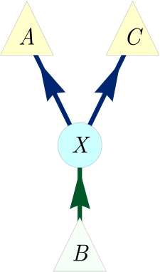
A causal structure that is compatible with any distribution
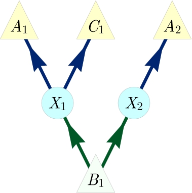
An inflation of Fig. 19.
While it is also not hard to write down the distribution constructed in the proof explicitly as
Appendix F Causal compatibility inequalities for the triangle scenario in machine-readable format
Table 2 lists the fifty two numerically irredundant polynomial inequalities resulting from consistent marginals of the Spiral inflation of Fig. 3. Stronger inequalities can be derived be considering larger inflations, such as the Web inflation of Fig. 2. Each row in the table specifies the coefficient of the corresponding correlator monomial. As noted previously, these inequalities also follow from the hypergraph transversals technique per Sec. 4.4.
A machine-readable and closed-under-symmetries version of the table in Sec. 4.3.
| constant | ||||||||||||||
| 1 | 0 | 0 | 0 | -1 | -1 | 0 | 0 | 0 | 0 | 1 | 0 | 0 | 0 | 0 |
| 1 | 0 | 0 | 0 | -1 | 1 | 0 | 0 | 0 | 0 | -1 | 0 | 0 | 0 | 0 |
| 1 | 0 | 0 | 0 | 1 | -1 | 0 | 0 | 0 | 0 | -1 | 0 | 0 | 0 | 0 |
| 1 | 0 | 0 | 0 | 1 | 1 | 0 | 0 | 0 | 0 | 1 | 0 | 0 | 0 | 0 |
| 1 | 0 | 0 | 0 | -1 | 0 | -1 | 0 | 0 | 1 | 0 | 0 | 0 | 0 | 0 |
| 1 | 0 | 0 | 0 | -1 | 0 | 1 | 0 | 0 | -1 | 0 | 0 | 0 | 0 | 0 |
| 1 | 0 | 0 | 0 | 1 | 0 | -1 | 0 | 0 | -1 | 0 | 0 | 0 | 0 | 0 |
| 1 | 0 | 0 | 0 | 1 | 0 | 1 | 0 | 0 | 1 | 0 | 0 | 0 | 0 | 0 |
| 1 | 0 | 0 | 0 | 0 | -1 | -1 | 0 | 1 | 0 | 0 | 0 | 0 | 0 | 0 |
| 1 | 0 | 0 | 0 | 0 | -1 | 1 | 0 | -1 | 0 | 0 | 0 | 0 | 0 | 0 |
| 1 | 0 | 0 | 0 | 0 | 1 | -1 | 0 | -1 | 0 | 0 | 0 | 0 | 0 | 0 |
| 1 | 0 | 0 | 0 | 0 | 1 | 1 | 0 | 1 | 0 | 0 | 0 | 0 | 0 | 0 |
| 3 | -1 | -1 | -1 | 2 | 2 | 2 | 1 | 1 | 1 | 1 | -1 | -1 | -1 | 1 |
| 3 | -1 | -1 | 1 | 2 | -2 | -2 | -1 | 1 | -1 | -1 | 1 | 1 | 1 | -1 |
| 3 | -1 | 1 | -1 | -2 | 2 | -2 | -1 | -1 | 1 | -1 | 1 | 1 | 1 | -1 |
| 3 | -1 | 1 | 1 | -2 | -2 | 2 | 1 | -1 | -1 | 1 | -1 | -1 | -1 | 1 |
| 3 | 1 | -1 | -1 | -2 | -2 | 2 | -1 | -1 | -1 | 1 | 1 | 1 | 1 | -1 |
| 3 | 1 | -1 | 1 | -2 | 2 | -2 | 1 | -1 | 1 | -1 | -1 | -1 | -1 | 1 |
| 3 | 1 | 1 | -1 | 2 | -2 | -2 | 1 | 1 | -1 | -1 | -1 | -1 | -1 | 1 |
| 3 | 1 | 1 | 1 | 2 | 2 | 2 | -1 | 1 | 1 | 1 | 1 | 1 | 1 | -1 |
| 4 | -2 | 0 | 0 | -3 | -2 | -2 | 1 | 1 | 0 | 2 | 1 | 1 | 0 | -1 |
| 4 | -2 | 0 | 0 | -3 | 2 | 2 | -1 | 1 | 0 | -2 | -1 | -1 | 0 | 1 |
| 4 | -2 | 0 | 0 | 3 | -2 | 2 | -1 | -1 | 0 | -2 | -1 | -1 | 0 | 1 |
| 4 | -2 | 0 | 0 | 3 | 2 | -2 | 1 | -1 | 0 | 2 | 1 | 1 | 0 | -1 |
| 4 | 2 | 0 | 0 | -3 | -2 | -2 | -1 | 1 | 0 | 2 | -1 | -1 | 0 | 1 |
| 4 | 2 | 0 | 0 | -3 | 2 | 2 | 1 | 1 | 0 | -2 | 1 | 1 | 0 | -1 |
| 4 | 2 | 0 | 0 | 3 | -2 | 2 | 1 | -1 | 0 | -2 | 1 | 1 | 0 | -1 |
| 4 | 2 | 0 | 0 | 3 | 2 | -2 | -1 | -1 | 0 | 2 | -1 | -1 | 0 | 1 |
| 4 | 0 | -2 | 0 | -2 | -2 | -3 | 1 | 0 | 2 | 1 | 0 | 1 | 1 | -1 |
| 4 | 0 | -2 | 0 | -2 | 2 | 3 | -1 | 0 | -2 | -1 | 0 | -1 | -1 | 1 |
| 4 | 0 | -2 | 0 | 2 | -2 | 3 | 1 | 0 | 2 | -1 | 0 | 1 | 1 | -1 |
| 4 | 0 | -2 | 0 | 2 | 2 | -3 | -1 | 0 | -2 | 1 | 0 | -1 | -1 | 1 |
| 4 | 0 | 2 | 0 | -2 | -2 | -3 | -1 | 0 | 2 | 1 | 0 | -1 | -1 | 1 |
| 4 | 0 | 2 | 0 | -2 | 2 | 3 | 1 | 0 | -2 | -1 | 0 | 1 | 1 | -1 |
| 4 | 0 | 2 | 0 | 2 | -2 | 3 | -1 | 0 | 2 | -1 | 0 | -1 | -1 | 1 |
| 4 | 0 | 2 | 0 | 2 | 2 | -3 | 1 | 0 | -2 | 1 | 0 | 1 | 1 | -1 |
| 4 | 0 | 0 | -2 | -2 | -3 | -2 | 1 | 2 | 1 | 0 | 1 | 0 | 1 | -1 |
| 4 | 0 | 0 | -2 | -2 | 3 | 2 | 1 | 2 | -1 | 0 | 1 | 0 | 1 | -1 |
| 4 | 0 | 0 | -2 | 2 | -3 | 2 | -1 | -2 | 1 | 0 | -1 | 0 | -1 | 1 |
| 4 | 0 | 0 | -2 | 2 | 3 | -2 | -1 | -2 | -1 | 0 | -1 | 0 | -1 | 1 |
| 4 | 0 | 0 | 2 | -2 | -3 | -2 | -1 | 2 | 1 | 0 | -1 | 0 | -1 | 1 |
| 4 | 0 | 0 | 2 | -2 | 3 | 2 | -1 | 2 | -1 | 0 | -1 | 0 | -1 | 1 |
| 4 | 0 | 0 | 2 | 2 | -3 | 2 | 1 | -2 | 1 | 0 | 1 | 0 | 1 | -1 |
| 4 | 0 | 0 | 2 | 2 | 3 | -2 | 1 | -2 | -1 | 0 | 1 | 0 | 1 | -1 |
| 4 | 0 | 0 | 0 | -2 | -2 | -2 | -1 | 2 | 2 | 2 | -1 | -1 | -1 | 0 |
| 4 | 0 | 0 | 0 | -2 | -2 | -2 | 1 | 2 | 2 | 2 | 1 | 1 | 1 | 0 |
| 4 | 0 | 0 | 0 | -2 | 2 | 2 | -1 | 2 | -2 | -2 | -1 | -1 | -1 | 0 |
| 4 | 0 | 0 | 0 | -2 | 2 | 2 | 1 | 2 | -2 | -2 | 1 | 1 | 1 | 0 |
| 4 | 0 | 0 | 0 | 2 | -2 | 2 | -1 | -2 | 2 | -2 | -1 | -1 | -1 | 0 |
| 4 | 0 | 0 | 0 | 2 | -2 | 2 | 1 | -2 | 2 | -2 | 1 | 1 | 1 | 0 |
| 4 | 0 | 0 | 0 | 2 | 2 | -2 | -1 | -2 | -2 | 2 | -1 | -1 | -1 | 0 |
| 4 | 0 | 0 | 0 | 2 | 2 | -2 | 1 | -2 | -2 | 2 | 1 | 1 | 1 | 0 |
Appendix G Recovering the Bell inequalities from the inflation technique
To further illustrate the power of the inflation technique, we now demonstrate how to recover all Bell inequalities [18], [20], [51] via our method. To keep things simple we only discuss the case of a bipartite Bell scenario with two values for both “settings” and “outcome” variables, but the case of more parties and/or more values per settings or outcome variable is totally analogous.
The causal structure associated to the Bell [17], [18], [20], [51] scenario [22 (Fig. E#2), 19 (Fig. 19), 33 (Fig. 1), 23 (Fig. 1), 52 (Fig. 2b), 53 (Fig. 2)] is depicted in Fig. 7. The observed variables are A, B, X, Y, and Λ is the latent common cause of A and B. One traditionally works with the conditional distribution
In the inflation of Fig. 8, the maximal ai-expressible sets are
where notably every maximal ai-expressible set contains all “settings” variables
By dividing each of the first four equations by the fifth, we obtain
The existence of a joint distribution of all six variables—i. e. the existence of a solution to the marginal problem—implies in particular
and similarly for the other three conditional distributions under consideration. For compatibility with the Bell scenario, Eq. (G.3) therefore implies that the original distribution must satisfy in particular
The possibility to write the conditional probabilities in the Bell scenario in this form is equivalent to the existence of a latent variable model, as noted in Fine’s theorem [122]. Thus, the existence of a solution to our marginal problem implies the existence of a latent variable model for the original distribution; the converse follows from our Lemma 4. Hence the inflation of Fig. 8 provides necessary and sufficient conditions for the compatibility of the original distribution with the Bell scenario.
Moreover, it is possible to describe the marginal polytope over the ai-expressible sets of Eq. (G.1), resulting in a concrete correspondence between tight Bell inequalities and the facets of our marginal polytope. This is based on the observation that the “settings” variables
where all six variables range over their possible values. Since the last four tensor factors occur in every direct summand in exactly the same way, we can also write such a polytope vertex as
in
and second the convex hull of all
This translates into the standard form of the CHSH inequality as follows. Upon using Eq. (G.3), the inequality becomes
so that dividing by the right-hand side results in one of the conventional forms of the CHSH inequality,
In conclusion, the inflation technique is powerful enough to get a precise characterization of all distributions compatible with the Bell causal structure, and our technique for generating polynomial inequalities through solving the marginal constraint problem recovers all Bell inequalities.
Some Bell inequalities may also be derived using the hypergraph transversals technique discussed in Sec. 4.4. For example, the inequality
is the inflationary precursor of the Bell inequality
as Eq. (G.7) is obtained from Eq. (G.6) by dividing both sides by

which corresponds to the original “Hardy paradox” [49] in our notation.
References
1. Pearl J. Causality: Models, reasoning, and inference. Cambridge University Press; 2009.10.1017/CBO9780511803161Suche in Google Scholar
2. Spirtes P, Glymour C, Scheines R. Causation, prediction, and search. Lecture Notes in Statistics. New York: Springer; 2011.Suche in Google Scholar
3. Studený M. Probabilistic conditional independence structures. Information Science and Statistics. London: Springer; 2005.Suche in Google Scholar
4. Koller D. Probabilistic graphical models: Principles and techniques. MIT Press; 2009.Suche in Google Scholar
5. Pearl J. Theoretical impediments to machine learning with seven sparks from the causal revolution. arXiv:1801.04016 (2018).10.1145/3159652.3176182Suche in Google Scholar
6. Rosset D, Gisin N, Wolfe E. Universal bound on the cardinality of local hidden variables in networks. Quantum Inf Comput 2018;18.10.26421/QIC18.11-12-2Suche in Google Scholar
7. Geiger D, Meek C. Graphical models and exponential families. In: Proc 14th conf uncert artif intell. AUAI; 1998. p. 156–65.Suche in Google Scholar
8. Lee CM, Spekkens RW. Causal inference via algebraic geometry: Feasibility tests for functional causal structures with two binary observed variables. J Causal Inference. 2017;5:20160013.10.1515/jci-2016-0013Suche in Google Scholar
9. Chaves R. Polynomial Bell inequalities. Phys Rev Lett. 2016;116:010402.10.1103/PhysRevLett.116.010402Suche in Google Scholar PubMed
10. Geiger D, Meek C. Quantifier elimination for statistical problems. In: Proc 15th conf uncert artif intell. AUAI; 1999. p. 226–35.Suche in Google Scholar
11. Garcia LD, Stillman M, Sturmfels B. Algebraic geometry of bayesian networks. J Symb Comput. 2005;39:331.10.1016/j.jsc.2004.11.007Suche in Google Scholar
12. Garcia LD. Algebraic statistics in model selection. In: Proc 20th conf uncert artif intell. AUAI; 2004. p. 177–84.Suche in Google Scholar
13. Garcia-Puente LD, Spielvogel S, Sullivant S. Identifying causal effects with computer algebra. In: Proc 26th conf uncert artif intell. AUAI; 2010. p. 193–200.Suche in Google Scholar
14. Tian J, Pearl J. On the testable implications of causal models with hidden variables. In: Proc 18th conf uncert artif intell. AUAI; 2002. p. 519–27.Suche in Google Scholar
15. Kang C, Tian J. Inequality constraints in causal models with hidden variables. In: Proc 22nd conf uncert artif intell. AUAI; 2006. p. 233–40.Suche in Google Scholar
16. Kang C, Tian J. Polynomial constraints in causal bayesian networks. In: Proc 23rd conf uncert artif intell. AUAI; 2007. p. 200–8.Suche in Google Scholar
17. Bell JS. On the Einstein-Podolsky-Rosen paradox. Physics. 1964;1:195.10.1103/PhysicsPhysiqueFizika.1.195Suche in Google Scholar
18. Clauser JF, Horne MA, Shimony A, Holt RA. Proposed experiment to test local hidden-variable theories. Phys Rev Lett. 1969;23:880.10.1103/PhysRevLett.23.880Suche in Google Scholar
19. Wood CJ, Spekkens RW. The lesson of causal discovery algorithms for quantum correlations: causal explanations of Bell-inequality violations require fine-tuning. New J Phys. 2015;17:033002.10.1088/1367-2630/17/3/033002Suche in Google Scholar
20. Brunner N, Cavalcanti D, Pironio S, Scarani V, Wehner S. Bell nonlocality. Rev Mod Phys. 2014;86:419.10.1103/RevModPhys.86.419Suche in Google Scholar
21. Fritz T. Beyond Bell’s theorem: correlation scenarios. New J Phys. 2012;14:103001.10.1088/1367-2630/14/10/103001Suche in Google Scholar
22. Henson J, Lal R, Pusey MF. Theory-independent limits on correlations from generalized Bayesian networks. New J Phys. 2014;16:113043.10.1088/1367-2630/16/11/113043Suche in Google Scholar
23. Fritz T. Beyond Bell’s theorem II: Scenarios with arbitrary causal structure. Commun Math Phys. 2015;341:391.10.1007/s00220-015-2495-5Suche in Google Scholar
24. Chaves R, Budroni C. Entropic nonsignaling correlations. Phys Rev Lett. 2016;116:240501.10.1103/PhysRevLett.116.240501Suche in Google Scholar PubMed
25. Chaves R, Luft L, Maciel TO, Gross D, Janzing D, Schölkopf B. Inferring latent structures via information inequalities. In: Proc 30th conf uncert artif intell. AUAI; 2014. p. 112–21.Suche in Google Scholar
26. Weilenmann M, Colbeck R. Non-Shannon inequalities in the entropy vector approach to causal structures. Quantum. 2018;2:57.10.22331/q-2018-03-14-57Suche in Google Scholar
27. Kela A, von Prillwitz K, Åberg J, Chaves R, Gross D. Semidefinite tests for latent causal structures. arXiv:1701.00652 (2017).Suche in Google Scholar
28. Tavakoli A, Skrzypczyk P, Cavalcanti D, Acín A. Nonlocal correlations in the star-network configuration. Phys Rev A. 2014;90:062109.10.1103/PhysRevA.90.062109Suche in Google Scholar
29. Rosset D, Branciard C, Barnea TJ, Pütz G, Brunner N, Gisin N. Nonlinear Bell inequalities tailored for quantum networks. Phys Rev Lett. 2016;116:010403.10.1103/PhysRevLett.116.010403Suche in Google Scholar PubMed
30. Tavakoli A. Bell-type inequalities for arbitrary noncyclic networks. Phys Rev A. 2016;93:030101.10.1103/PhysRevA.93.030101Suche in Google Scholar
31. Pearl J. On the Testability of Causal Models with Latent and Instrumental Variables. In: Proc 11th conf uncert artif intell. AUAI; 1995. p. 435–43.Suche in Google Scholar
32. Steudel B, Ay N. Information-theoretic inference of common ancestors. Entropy. 2015;17:2304.10.3390/e17042304Suche in Google Scholar
33. Chaves R, Luft L, Gross D. Causal structures from entropic information: geometry and novel scenarios. New J Phys. 2014;16:043001.10.1088/1367-2630/16/4/043001Suche in Google Scholar
34. Evans RJ. Graphical methods for inequality constraints in marginalized DAGs. In: Proc 2012 IEEE intern work MLSP. IEEE; 2012. p. 1–6.10.1109/MLSP.2012.6349796Suche in Google Scholar
35. Fritz T, Chaves R. Entropic inequalities and marginal problems. IEEE Trans Inf Theory. 2013;59:803.10.1109/TIT.2012.2222863Suche in Google Scholar
36. Pienaar J. Which causal structures might support a quantum–classical gap? New J Phys. 2017;19:043021.10.1088/1367-2630/aa673eSuche in Google Scholar
37. Braunstein SL, Caves CM. Information-theoretic Bell inequalities. Phys Rev Lett. 1988;61:662.10.1103/PhysRevLett.61.662Suche in Google Scholar PubMed
38. Schumacher BW. Information and quantum nonseparability. Phys Rev A. 1991;44:7047.10.1103/PhysRevA.44.7047Suche in Google Scholar
39. Leifer MS, Spekkens RW. Towards a formulation of quantum theory as a causally neutral theory of Bayesian inference. Phys Rev A. 2013;88:052130.10.1103/PhysRevA.88.052130Suche in Google Scholar
40. Chaves R, Majenz C, Gross D. Information–theoretic implications of quantum causal structures. Nat Commun. 2015;6:5766.10.1038/ncomms6766Suche in Google Scholar PubMed
41. Ried K, Agnew M, Vermeyden L, Janzing D, Spekkens RW, Resch KJ. A quantum advantage for inferring causal structure. Nat Phys. 2015;11:414.10.1038/nphys3266Suche in Google Scholar
42. Costa F, Shrapnel S. Quantum causal modelling. New J Phys. 2016;18:063032.10.1088/1367-2630/18/6/063032Suche in Google Scholar
43. Allen J-MA, Barrett J, Horsman DC, Lee CM, Spekkens RW. Quantum common causes and quantum causal models. Phys Rev X. 2017;7:031021.10.1103/PhysRevX.7.031021Suche in Google Scholar
44. Hardy L. Quantum theory from five reasonable axioms, quant-ph/0101012 (2001).Suche in Google Scholar
45. Barrett J. Information processing in generalized probabilistic theories. Phys Rev A. 2007;75:032304.10.1103/PhysRevA.75.032304Suche in Google Scholar
46. Boldi P, Vigna S. Fibrations of graphs. Discrete Math. 2002;243:21.10.1016/S0012-365X(00)00455-6Suche in Google Scholar
47. Branciard C, Rosset D, Gisin N, Pironio S. Bilocal versus nonbilocal correlations in entanglement-swapping experiments. Phys Rev A. 2012;85:032119.10.1103/PhysRevA.85.032119Suche in Google Scholar
48. Dür W, Vidal G, Cirac JI. Three qubits can be entangled in two inequivalent ways. Phys Rev A. 2000;62:062314.10.1103/PhysRevA.62.062314Suche in Google Scholar
49. Hardy L. Nonlocality for two particles without inequalities for almost all entangled states. Phys Rev Lett. 1993;71:1665.10.1103/PhysRevLett.71.1665Suche in Google Scholar PubMed
50. Mansfield S, Fritz T. Hardy’s non-locality paradox and possibilistic conditions for non-locality. Found Phys. 2012;42:709.10.1007/s10701-012-9640-1Suche in Google Scholar
51. Bell JS. On the problem of hidden variables in quantum mechanics. Rev Mod Phys. 1966;38:447.10.1103/RevModPhys.38.447Suche in Google Scholar
52. Donohue JM, Wolfe E. Identifying nonconvexity in the sets of limited-dimension quantum correlations. Phys Rev A. 2015;92:062120.10.1103/PhysRevA.92.062120Suche in Google Scholar
53. Steeg GV, Galstyan A. A sequence of relaxations constraining hidden variable models. In: Proc 27th conf uncert artif intell. AUAI; 2011. p. 717–26.Suche in Google Scholar
54. Cirel’son BS. Quantum generalizations of Bell’s inequality. Lett Math Phys. 1980;4:93. Available at http://www.tau.ac.il/~tsirel/download/qbell80.html.10.1007/BF00417500Suche in Google Scholar
55. Popescu S, Rohrlich D. Quantum nonlocality as an axiom. Found Phys. 1994;24:379.10.1007/BF02058098Suche in Google Scholar
56. Barrett J, Pironio S. Popescu-Rohrlich correlations as a unit of nonlocality. Phys Rev Lett. 2005;95:140401.10.1103/PhysRevLett.95.140401Suche in Google Scholar PubMed
57. Liang Y-C, Spekkens RW, Wiseman HM. Specker’s parable of the overprotective seer: A road to contextuality, nonlocality and complementarity. Phys Rep. 2011;506:1.10.1016/j.physrep.2011.05.001Suche in Google Scholar
58. Roberts D. Aspects of quantum non-locality. PhD thesis. University of Bristol; 2004.Suche in Google Scholar
59. Pitowsky I. George Boole’s ‘Conditions of possible experience’ and the quantum puzzle. Br J Philos Sci. 1994;45:95.10.1093/bjps/45.1.95Suche in Google Scholar
60. Pitowsky I. Quantum probability – Quantum logic. Lecture Notes in Physics. vol. 321. Springer-Verlag; 1989.Suche in Google Scholar
61. Kellerer HG. Verteilungsfunktionen mit gegebenen Marginalverteilungen. Z Wahrscheinlichkeitstheorie. 1964;3:247.10.1007/BF00534912Suche in Google Scholar
62. Leggett AJ, Garg A. Quantum mechanics versus macroscopic realism: is the flux there when nobody looks? Phys Rev Lett. 1985;54:857.10.1103/PhysRevLett.54.857Suche in Google Scholar PubMed
63. Araújo M, Túlio Quintino M, Budroni C, Terra Cunha M, Cabello A. All noncontextuality inequalities for the n-cycle scenario. Phys Rev A. 2013;88:022118.10.1103/PhysRevA.88.022118Suche in Google Scholar
64. Horodecki R, Horodecki P, Horodecki M, Horodecki K. Quantum entanglement. Rev Mod Phys. 2009;81:865.10.1103/RevModPhys.81.865Suche in Google Scholar
65. Abramsky S, Brandenburger A. The sheaf-theoretic structure of non-locality and contextuality. New J Phys. 2011;13:113036.10.1088/1367-2630/13/11/113036Suche in Google Scholar
66. Vorob’ev NN. Consistent families of measures and their extensions. Theory Probab Appl. 1960;7:147.10.1137/1107014Suche in Google Scholar
67. Budroni C, Miklin N, Chaves R. Indistinguishability of causal relations from limited marginals. Phys Rev A. 2016;94:042127.10.1103/PhysRevA.94.042127Suche in Google Scholar
68. Kahle T. Neighborliness of marginal polytopes. Beitr Algebra Geom. 2010;51:45.Suche in Google Scholar
69. Andersen ED. Certificates of primal or dual infeasibility in linear programming. Comput Optim Appl. 2001;20:171.10.1023/A:1011259103627Suche in Google Scholar
70. Garuccio A. Hardy’s approach, Eberhard’s inequality, and supplementary assumptions. Phys Rev A. 1995;52:2535.10.1103/PhysRevA.52.2535Suche in Google Scholar
71. Cabello A. Bell’s theorem with and without inequalities for the three-qubit Greenberger-Horne-Zeilinger and W states. Phys Rev A. 2002;65:032108.10.1103/PhysRevA.65.032108Suche in Google Scholar
72. Braun D, Choi M-S. Hardy’s test versus the Clauser-Horne-Shimony-Holt test of quantum nonlocality: Fundamental and practical aspects. Phys Rev A. 2008;78:032114.10.1103/PhysRevA.78.032114Suche in Google Scholar
73. Mančinska L, Wehner S. A unified view on Hardy’s paradox and the Clauser–Horne–Shimony–Holt inequality. J Phys A. 2014;47:424027.10.1088/1751-8113/47/42/424027Suche in Google Scholar
74. Ghirardi G, Marinatto L. Proofs of nonlocality without inequalities revisited. Phys Lett A. 2008;372:1982.10.1016/j.physleta.2007.11.012Suche in Google Scholar
75. Eiter T, Makino K, Gottlob G. Computational aspects of monotone dualization: A brief survey. Discrete Appl Math. 2008;156:2035.10.1016/j.dam.2007.04.017Suche in Google Scholar
76. Barrett C, Fontaine P, Tinelli C. The satisfiability modulo theories library. 2016. www.SMT-LIB.org.Suche in Google Scholar
77. Fordan A. Projection in constraint logic programming. Ios Press; 1999.Suche in Google Scholar
78. Dantzig GB, Eaves BC. Fourier-Motzkin elimination and its dual. J Comb Theory, Ser A. 1973;14:288.10.1016/0097-3165(73)90004-6Suche in Google Scholar
79. Bastrakov SI, Zolotykh NY. Fast method for verifying Chernikov rules in Fourier-Motzkin elimination. Comput Math Math Phys. 2015;55:160.10.1134/S0965542515010042Suche in Google Scholar
80. Balas E. Projection with a minimal system of inequalities. Comput Optim Appl. 1998;10:189.10.21236/ADA257237Suche in Google Scholar
81. Jones CN, Kerrigan EC, Maciejowski JM. On polyhedral projection and parametric programming. J Optim Theory Appl. 2008;138:207.10.1007/s10957-008-9384-4Suche in Google Scholar
82. Jones C. Polyhedral tools for control. PhD thesis. University of Cambridge; 2005.Suche in Google Scholar
83. Jones C, Kerrigan EC, Maciejowski J. Equality set projection: A new algorithm for the projection of polytopes in halfspace representation. Tech Rep. Cambridge University Engineering Dept; 2004.Suche in Google Scholar
84. Spekkens RW. The paradigm of kinematics and dynamics must yield to causal structure. In: Questioning the foundations of physics: which of our fundamental assumptions are wrong? Springer International; 2015. p. 5–16.10.1007/978-3-319-13045-3_2Suche in Google Scholar
85. Henson J. Causality, Bell’s theorem, and ontic definiteness. arXiv:1102.2855 (2011).Suche in Google Scholar
86. Barrett J, Linden N, Massar S, Pironio S, Popescu S, Roberts D. Nonlocal correlations as an information-theoretic resource. Phys Rev A. 2005;71:022101.10.1103/PhysRevA.71.022101Suche in Google Scholar
87. Scarani V. The device-independent outlook on quantum physics. Acta Phys Slovaca. 2012;62:347.Suche in Google Scholar
88. Bancal J-D. On the device-independent approach to quantum physics. Springer International; 2014.10.1007/978-3-319-01183-7Suche in Google Scholar
89. Chaves R, Fritz T. Entropic approach to local realism and noncontextuality. Phys Rev A. 2012;85:032113.10.1103/PhysRevA.85.032113Suche in Google Scholar
90. Barnum H, Wilce A. Post-classical probability theory. arXiv:1205.3833 (2012).Suche in Google Scholar
91. Janotta P, Hinrichsen H. Generalized probability theories: what determines the structure of quantum theory? J Phys A. 2014;47:323001.10.1088/1751-8113/47/32/323001Suche in Google Scholar
92. Fraser TC, Wolfe E. Causal compatibility inequalities admitting quantum violations in the triangle structure. Phys Rev A. 2018;98:022113.10.1103/PhysRevA.98.022113Suche in Google Scholar
93. Barnum H, Caves CM, Fuchs CA, Jozsa R, Schumacher B. Noncommuting mixed states cannot be broadcast. Phys Rev Lett. 1996;76:2818.10.1103/PhysRevLett.76.2818Suche in Google Scholar PubMed
94. Barnum H, Barrett J, Leifer M, Wilce A. Cloning and broadcasting in generic probabilistic theories. quant-ph/0611295 (2006).Suche in Google Scholar
95. Popescu S. Nonlocality beyond quantum mechanics. Nat Phys. 2014;10:264.10.1038/nphys2916Suche in Google Scholar
96. Yang TH, Navascués M, Sheridan L, Scarani V. Quantum Bell inequalities from macroscopic locality. Phys Rev A. 2011;83:022105.10.1103/PhysRevA.83.022105Suche in Google Scholar
97. Rohrlich D. PR-box correlations have no classical limit. In: Quantum theory: A two-time success story. Milan: Springer; 2014. p. 205–11.10.1007/978-88-470-5217-8_13Suche in Google Scholar
98. Pawlowski M, Scarani V. Information causality. arXiv:1112.1142 (2011).Suche in Google Scholar
99. Fritz T, Sainz AB, Augusiak R, Brask JB, Chaves R, Leverrier A, Acin A. Local orthogonality as a multipartite principle for quantum correlations. Nat Commun. 2013;4:2263.10.1038/ncomms3263Suche in Google Scholar PubMed
100. Sainz AB, Fritz T, Augusiak R, Brask JB, Chaves R, Leverrier A, Acín A. Exploring the local orthogonality principle. Phys Rev A. 2014;89:032117.10.1103/PhysRevA.89.032117Suche in Google Scholar
101. Cabello A. Simple explanation of the quantum limits of genuine n-body nonlocality. Phys Rev Lett. 2015;114:220402.10.1103/PhysRevLett.114.220402Suche in Google Scholar PubMed
102. Barnum H, Müller MP, Ududec C. Higher-order interference and single-system postulates characterizing quantum theory. New J Phys. 2014;16:123029.10.1088/1367-2630/16/12/123029Suche in Google Scholar
103. Navascués M, Guryanova Y, Hoban MJ, Acín A. Almost quantum correlations. Nat Commun. 2015;6:6288.10.1038/ncomms7288Suche in Google Scholar PubMed
104. Kang C, Tian J. Polynomial constraints in causal bayesian networks. In: Proc 23rd conf uncert artif intell. AUAI; 2007. p. 200–8.Suche in Google Scholar
105. Navascués M, Pironio S, Acín A. A convergent hierarchy of semidefinite programs characterizing the set of quantum correlations. New J Phys. 2008;10:073013.10.1088/1367-2630/10/7/073013Suche in Google Scholar
106. Pál KF, Vértesi T. Quantum bounds on Bell inequalities. Phys Rev A. 2009;79:022120.10.1103/PhysRevA.79.022120Suche in Google Scholar
107. Wolfe E, et al. Quantum inflation: A general approach to quantum causal compatibility (in preparation).Suche in Google Scholar
108. Navascués M, Wolfe E. The inflation technique completely solves the causal compatibility problem. arXiv:1707.06476 (2017).Suche in Google Scholar
109. Avis D, Bremner D, Seidel R. How good are convex hull algorithms? Comput Geom. 1997;7:265.10.1145/220279.220282Suche in Google Scholar
110. Fukuda K, Prodon A. Double description method revisited. In: Combin & Comp Sci. Springer-Verlag; 1996. p. 91–111.10.1007/3-540-61576-8_77Suche in Google Scholar
111. Shapot DV, Lukatskii AM. Solution building for arbitrary system of linear inequalities in an explicit form. Am J Comput Math. 2012;02:1.10.4236/ajcm.2012.21001Suche in Google Scholar
112. Avis D. A revised implementation of the reverse search vertex enumeration algorithm. In: Polytopes — Combinatorics and computation. DMV Seminar. vol. 29. Basel: Birkhäuser; 2000. p. 177–98.10.1007/978-3-0348-8438-9_9Suche in Google Scholar
113. Gläßle T, Gross D, Chaves R. Computational tools for solving a marginal problem with applications in Bell non-locality and causal modeling. J Phys A. 2018;51:484002.10.1088/1751-8121/aae754Suche in Google Scholar
114. Bremner D, Sikiric MD, Schürmann A. Polyhedral representation conversion up to symmetries. In: Polyhedral computation. CRM proc lecture notes, vol. 48. Amer Math Soc; 2009. p. 45–71.10.1090/crmp/048/03Suche in Google Scholar
115. Schürmann A. Exploiting symmetries in polyhedral computations. Disc Geom Optim. 2013;265.10.1007/978-3-319-00200-2_15Suche in Google Scholar
116. Kaibel V, Liberti L, Schürmann A, Sotirov R. Mini-workshop: Exploiting symmetry in optimization. Oberwolfach Rep. 2010;7:2245.10.4171/OWR/2010/38Suche in Google Scholar
117. Rehn T, Schürmann A. C++ tools for exploiting polyhedral symmetries. In: Proc 3rd int congr conf math soft, ICMS’10. Springer-Verlag; 2010. p. 295–8.10.1007/978-3-642-15582-6_48Suche in Google Scholar
118. Lörwald S, Reinelt G. PANDA: a software for polyhedral transformations. EURO J Comp Optim. 2015;3:297.10.1007/s13675-015-0040-0Suche in Google Scholar
119. Yeung RW. Beyond Shannon-type inequalities. In: Information theory and network coding. Springer US; 2008. p. 361–86.10.1007/978-0-387-79234-7_15Suche in Google Scholar
120. Kaced T. Equivalence of two proof techniques for non-Shannon-type inequalities. In: Information theory proceedings (ISIT). IEEE; 2013. p. 236–40.10.1109/ISIT.2013.6620223Suche in Google Scholar
121. Dougherty R, Freiling CF, Zeger K. Non-Shannon information inequalities in four random variables. arXiv:1104.3602 (2011).Suche in Google Scholar
122. Fine A. Hidden variables, joint probability, and the Bell inequalities. Phys Rev Lett. 1982;48:291.10.1103/PhysRevLett.48.291Suche in Google Scholar
123. Namioka I, Phelps R. Tensor products of compact convex sets. Pac J Math. 1969;31:469.10.2140/pjm.1969.31.469Suche in Google Scholar
124. Bogart T, Contois M, Gubeladze J. Hom-polytopes. Math Z. 2013;273:1267.10.1007/s00209-012-1053-5Suche in Google Scholar
© 2019 Walter de Gruyter GmbH, Berlin/Boston
This article is distributed under the terms of the Creative Commons Attribution Non-Commercial License, which permits unrestricted non-commercial use, distribution, and reproduction in any medium, provided the original work is properly cited.
Artikel in diesem Heft
- Research Articles
- Technical Considerations in the Use of the E-Value
- Regression Adjustments for Estimating the Global Treatment Effect in Experiments with Interference
- The Inflation Technique for Causal Inference with Latent Variables
- A Gaussian Process Framework for Overlap and Causal Effect Estimation with High-Dimensional Covariates
- Causal, Casual and Curious
- Sufficient Causes: On Oxygen, Matches, and Fires