Data on Repeated Offerings in the German Housing Market Based on RWI-GEO-RED
-
Philipp Breidenbach
 ,
Lukas Hoernig
,
Lukas Hoernig
 and
Thorben Wiebe
and
Thorben Wiebe

Abstract
This paper introduces a repeated-sales algorithm tailored for the German real estate market, addressing the lack of such data. Utilizing the dataset RWI-GEO-RED from FDZ Ruhr at RWI, which exploits data from ImmobilienScout24.de, the algorithm classifies repeat-sales and repeat-rent listings, overcoming challenges like measurement errors and deviations in property characteristics. The methodology, based on nearest centroid classification, ensures accurate clustering of similar listings. The paper compares the new repeated-sales indices with the traditional hedonic price index, revealing more conservative estimates of rent growth. Additionally, the data’s panel structure allows for detailed analysis of unit-level dynamics and mispricing. The study highlights the advantages of this approach and suggests potential research avenues, providing a valuable tool for economists and policymakers to assess housing market trends in Germany.
1 Introduction
Expenditure on housing costs dominates the expenditure structure of most households, both in terms of monthly rent payments and, in many cases, the cost of property financing. Turning to assets, for most owner-occupied households, housing is the largest household asset. Individual households (as current or potential future owners) tend to pay close attention to changes in house prices that affect wealth or affordability respectively (OECD et al. 2013). Because of its importance in terms of costs and assets, real estate price research is therefore a well-established topic in many economic research papers.
Here, residential property price indices (RPPIs) play an essential role, serving economists and policy makers as an indicator of financial soundness and a variety of other economic activities. By its very nature, housing is a highly heterogeneous good without a single observable market price (Leishman and Watkins 2002). Thus, attempts to transform information on properties with a variety of price-determining characteristics into a single representative measure face a number of obstacles. A perennial problem in the construction of RPPIs is differences in the quality of the characteristics (Englund, Quigley, and Redfearn 1998; Greenlees 1982; Kirby-McGregor and Martin 2019). These differences are of two types: improvements and depreciation. In times of an increasing need for energy renovations to impede climate change, the former has only gained in relevance. More generally, price movements due to quality changes needs to be disentangled from purely time-related movements in order to allow unbiased comparisons.
To achieve this, the repeated-sales methodology exploits multiple sales of the same unit over time and calculates the price difference between sales as the constant quality price movement of the unit. This approach attempts to control for time-invariant unobserved/unobservable differences in quality between properties, a problem that typically arises when using hedonic models (Englund, Quigley, and Redfearn 1998; Nagaraja, Brown, and Wachter 2014), e.g. curb appeal or the quality of landscaping (Bajari et al. 2012). First proposed by Bailey, Muth, and Nourse (1963, geometric repeated sales-index, GRS) and later adapted by Shiller (1991, arithmetic repeated-sales index, ARS), the methodology is widely used in past and current literature and is even referred to as the “the gold standard in house price construction” (Ahlfeldt, Heblich, and Seidel 2023, p. 1). In the context of Germany, however, no data are available to construct such indices and thus no opportunity exists for research to benefit from the potential advantages of this methodology. In this paper, we propose an algorithm to classify repeat-sales and repeat-rent in the German real estate market, based on information on real estate listings obtained from Germany’s largest real estate listing website, ImmobilienScout24.de, thus filling the gap in the literature.
The article is structured as follows: Section 2 describes the data basis and the algorithm, while Section 3 shows descriptive statistics of the resulting data and uses them to construct indices. Thereafter, Section 4 outlines some advantages of the data and suggests potential research avenues. Section 5 concludes with information on how to access the data.
2 Repeated Sales Classification
2.1 Data Basis
We use the RWI-GEO-RED data (RWI, ImmobilienScout24 2023a, 2023b, 2023c) as the basis for applying our algorithm. The data include all listings published on Germany’s largest real estate listing website ImmobilienScout24.de, which has a self-reported market share of about 50 % (Georgi and Barkow 2010). The listings contain both apartments and houses for residential use in Germany, either for sale or for rent. Owners or real estate agents are required to provide information on key criteria to place the ad, such as rent/price, square footage, floor(s) and number of rooms. They can further increase their searchability, and therefore their chances/time to sell or rent, by providing optional information, such as whether the unit has a garden or basement.[1] The original data covers the years from 2007 to 2023 on a monthly level and provides information on the exact geographical location of the unit.
These characteristics lend themselves well to the implementation of the proposed algorithm, as both the presence of mandatory base information and the units point coordinate allow for a sharp classification of clusters.
2.2 Algorithm
The employed algorithm is a customized variant of a nearest centroid classifier of the nearest neighbors family. Based on the centroid, which is chosen by the algorithm and converted into the cluster identifier, the individual unit listings are uniquely sorted into related/similar clusters.
In general, all listings are subject to slight deviations resulting from either measurement error, calculation error, user error or a combination of all three. For example, suppose a unit is listed twice, but once the living space was measured by the user manually and once it was calculated based on the floor plan. The challenge here is to separate listings that refer to the same unit but have slight variations in characteristics from those that refer to a completely different unit.
Algorithm 1:
Centroid candidacy.
| Require: N coord > 0 |
| ω k = [LS k , R k , F k ] with k ∈ (i, j) |
| for i, j in N coord do |
| Ω k = scale(ω k ) with k ∈ (i, j) |
| if Ω i ≅Ω j then ⊳ ≅ → is similar, see text for details. |
| i candidate centroid of j |
|
|
| else |
| i not centroid of j |
| SimDistance ij = -1 |
| end if |
| end for |
To address this challenge, we calculate the similarity of each listing i to every other listing j at the level of point coordinates (N coord ), see Algorithm 1. Specifically, we consider the Euclidean distance SimDistance ij between the listings scaled by the mandatory characteristics Ω k , i.e ω k : living space (LS) number of rooms (R) and floor (F).[2] This procedure transforms the Euclidean distance into a relative percentage difference, which makes it easier to interpret and is used to resolve conflicting classifications in the second step. However, before proceeding to the actual classification, we impose additional constrains on the characteristics to limit the range of possible matches: To be considered as a possible cluster of the respective centroid i, the other listings j must be within the 5 % interval of LS, within 0.5 of R and exactly match R. In addition, we use the presence of a balcony to pre-split the point coordinate into two groups. Listings that do not meet these conditions are assigned -1 by default. This not only decreases the number of required permutations, but also prevents grouping of unlikely matches, suhc as identical apartments on different floors.
Repeating this process for all of the listings on the point coordinate results in a N coord xN coord matrix, pertaining the SimDistance ij if the conditions are met, and -1 otherwise. This matrix builds the core part in the next step, see Algorithm 2, when deciding on which clusters to choose and how to resolve conflicts. In particular, there are two possible conflicts emerging:
First, a member i can be a possible match to several centroid candidates l, j. Resolving this conflict is straightforward, since we want to group the most similar listings together, we can choose the cluster Θ with the lowest SimDistance.
Second, a member i may be a possible match to a centroid candidate j, while at the same time being selected as a centroid candidate by the same or another member j. This conflict occurs, for example, in listings with overlapping intervals, where the listings simultaneously chose each other as both centroid and member. Here, the above consideration of choosing the most similar listings falls short, since the costs of the options are not equivalent. When i is chosen as a member instead of a centroid, the cost is to the entire cluster of listings Θ, not just to the individual listing itself. To account for this, we compare the average SimDistance within the cluster (L ij ), excluding the SimDistance of the centroid itself, since it is zero by definition, with the SimDistance that would result if the centroid were a member instead (L ji ). This comparison allows us to choose the configuration that maximizes the similarity gain.
Algorithm 2:
Centroid selection.
| Require: SimDistance ij ≠ -1 |
| switch i do |
| case SimDistance ij ≠ -1 and SimDistance il ≠ -1 ⊳ multiple centroid candidates |
| Θ ijl = arg min(SimDistance ij , SimDistance il ) |
| case SimDistance ij ≠ -1 and SimDistance ji ≠ -1 ⊳ conflicting member and centroid |
| Θ ij = arg min(L ij , L ji ) |
| with L
ij
=
|
| with L ji = SimDistance ji |
| case TRUE ⊳ default without conflicts |
| Θ ij = SimDistance ij |
| end switch |
3 Descriptive Statistics and Application
As mentioned above, a popular application of repeated sales data is the construction of price indices. In this section we compare the hedonic price index, the current standard for Germany, with the repeated sales indices (Bailey, Muth, and Nourse 1963; Shiller 1991), whose construction is enabled by the new data. To ensure comparability, the data for both indices are prepared in the same way, following Thiel (2024b). This RWI-GEO-REDX dataset on housing price index is described in Klick and Schaffner (2021). In addition, the quarterly index values are based on the first quarter of 2010 to allow for comparison of values over different magnitudes. Therefore, each change is expressed in percentage points relative to the corresponding base year values.
Figure 1 shows the different price indices for apartment rents in Germany between 2010 and 2023. The hedonic index (blue) shows the strongest upward trend, indicating a rent increase of about 72 percentage points. The repeated sales indices, ARS (red) and GRS (green), paint a more conservative picture of total rent growth over the time horizon, suggesting growth of 44 and 46 percentage points, respectively. Nevertheless, the overall trend is very similar. All of the price indices show a monotonic increasing trend, where the growth is slowing down, but still remains positive around 2015 and 2020.
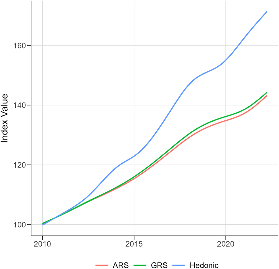
Price indices for Germany – apartment rent. Notes: Illustration of quarterly price indices based in the first quarter of 2010. Source: Authors’ graph.
This pattern is confirmed when zooming into the exemplary cities of Berlin, Frankfurt, and Munich in Figure 2. The cities are colored as indicated in the figure legend, where the dotted line shows the hedonic and the solid line the GRS value. For each city, the hedonic measure indicates a larger growth, while the GRS estimate the price increase more conservatively.
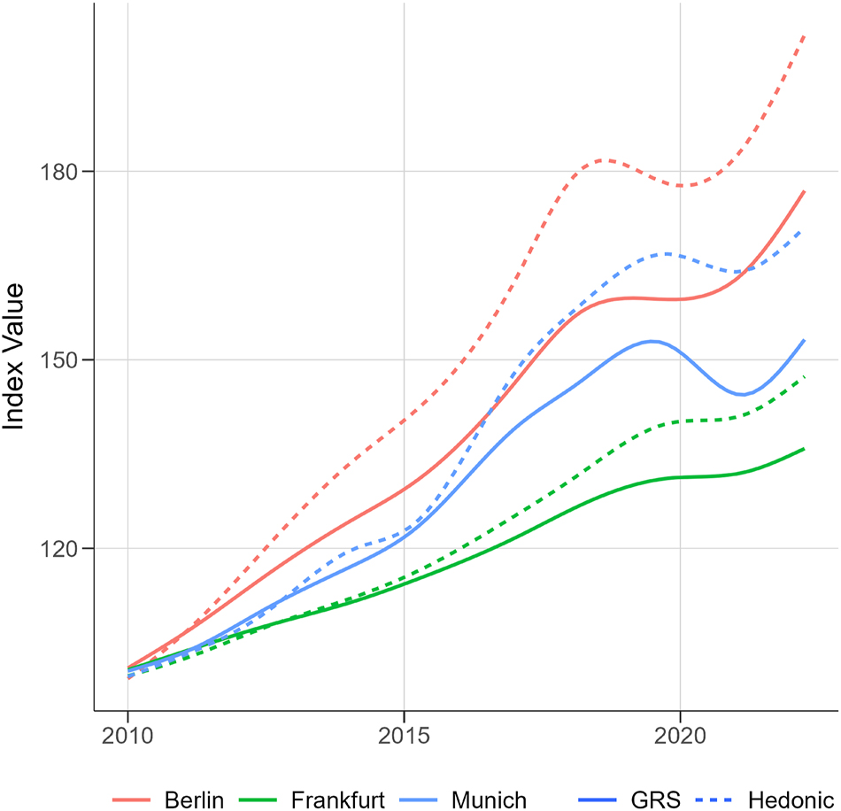
Price indices for selected cities – apartment rent. Notes: Illustration of quarterly price indices based in the first quarter of 2010. Source: Authors’ graph.
In Figure 3, we repeat the illustration of the three indices for apartment sales instead of apartment rents. Again, the pattern is repeated, with monotonic increases in all three measures. While the hedonic index still shows the largest growth rates, the difference is considerably smaller in magnitude. Notably, the growth rates for apartment sales do not seem to have experienced a periodic slowdown, but rather an ever-increasing trend.
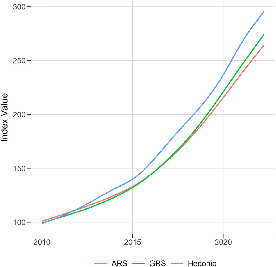
Price indices for Germany – apartment sales. Notes: Illustration of quarterly price indices based in the first quarter of 2010. Source: Authors’ graph.
4 Advantages and Research Avenues
The extended data offer two main advantages to researchers. First, the construction of price indices similar to those described above for different regional units. Second, the emergent panel structure resulting from the clustering of the longitudinal data. This allows the study of common and individual dynamics of units, such as listing updates as well as mispricing (Knight 2002; Knight, Sirmans, and Turnbull 1994; Lyons 2015). Furthermore, it allows for unit-level fixed effects to be included in models. This is much more precise than other common alternatives, such as grid-level fixed effects, and can therefore control for a much more detailed range of unobserved/unobservable heterogeneity. For example, the fact that an apartment faces north and therefore has little natural light cannot be observed by the researcher, but it can reduce the value of the apartment.
5 Data Availability
The variables introduced by the algorithm will be added to future releases of the RWI-GEO-RED data, while the code can be found at [GitHub].[3] The data are available to researchers for non-commercial use. There are two versions of the RWI-GEO-RED data. First, the Scientific Use Files (SUF) cover all information except the exact geo-coordinates. Second, the full datasets are available in the Data Secure Room of the FDZ Ruhr in Essen (on-site access).[4] The data can be obtained as a Stata datasets (.dta), .csv files, andparquet files. Data access to both versions requires a signed data use agreement. Both versions are restricted to non-commercial research and only researchers of scientific institutions are eligible to apply for data access. The SUF may be used at the workplace of the users. Data access is provided by the Research Data Centre Ruhr at the RWI – Leibniz-Institute for Economic Research (FDZ Ruhr). The data can be accessed at the data access website of FDZ Ruhr.[5] The application form includes a brief description and title of the project, information on the applying department, expected duration of data usage as well as further participants in the project. Data users shall cite the datasets properly with the respective DOIs.
References
Ahlfeldt, G. M., S. Heblich, and T. Seidel. 2023. “Micro-geographic Property Price and Rent Indices.” Regional Science and Urban Economics 98: 103836. https://doi.org/10.1016/j.regsciurbeco.2022.103836.Search in Google Scholar
Bailey, M. J., R. F. Muth, and H. O. Nourse. 1963. “A Regression Method for Real Estate Price Index Construction.” Journal of the American Statistical Association 58 (304): 933–42. https://doi.org/10.1080/01621459.1963.10480679.Search in Google Scholar
Bajari, P., J. C. Fruehwirth, K. I. Kim, and C. Timmins. 2012. “A Rational Expectations Approach to Hedonic Price Regressions with Time-Varying Unobserved Product Attributes: The Price of Pollution.” The American Economic Review 102 (5): 1898–926. https://doi.org/10.1257/aer.102.5.1898.Search in Google Scholar
Englund, P., J. M. Quigley, and C. L. Redfearn. 1998. “Improved Price Indexes for Real Estate: Measuring the Course of Swedish Housing Prices.” Journal of Urban Economics 44 (2): 171–96. https://doi.org/10.1006/juec.1997.2062.Search in Google Scholar
Georgi, S., and P. Barkow. 2010. “Wohnimmobilien-indizes: Vergleich Deutschland–Großbritannien [residential Real Estate Indices–A Comparison between germany and the uk].” ZIA Projektbericht.Search in Google Scholar
Greenlees, J. S. 1982. “An Empirical Evaluation of the Cpi Home Purchase Index, 1973–1978.” Real Estate Economics 10 (1): 1–24. https://doi.org/10.1111/1540-6229.00255.Search in Google Scholar
Kirby-McGregor, M., and S. Martin. 2019. “An R Package for Calculating Repeat-Sale Price Indices.” Romanian Statistical Review (3).Search in Google Scholar
Klick, L., and S. Schaffner. 2021. “Jahrbücher für Nationalökonomie und Statistik.” 241 (1): 119–29. https://doi.org/10.1515/jbnst-2020-0001.Search in Google Scholar
Knight, J. R. 2002. “Listing Price, Time on Market, and Ultimate Selling Price: Causes and Effects of Listing Price Changes.” Real Estate Economics 30 (2): 213–37. https://doi.org/10.1111/1540-6229.00038.Search in Google Scholar
Knight, J. R., C. Sirmans, and G. K. Turnbull. 1994. “List Price Signaling and Buyer Behavior in the Housing Market.” Journal of Real Estate Finance and Economics 9: 177–92. https://doi.org/10.1007/bf01099271.Search in Google Scholar
Leishman, C., and C. Watkins. 2002. “Estimating Local Repeat Sales House Price Indices for British Cities.” Journal of Property Investment & Finance 20 (1): 36–58. https://doi.org/10.1108/14635780210416255.Search in Google Scholar
Lyons, R. C. 2015. “East, West, Boom and Bust: The Spread of House Prices and Rents in Ireland, 2007–2012.” Journal of Property Research 32 (1): 77–101. https://doi.org/10.1080/09599916.2013.870922.Search in Google Scholar
Nagaraja, C., L. Brown, and S. Wachter. 2014. “Repeat Sales House Price Index Methodology.” Journal of Real Estate Literature 22 (1): 23–46. https://doi.org/10.1080/10835547.2014.12090375.Search in Google Scholar
OECD, I. L., I. M. Fund, T. W. Bank, and U. N. E. C. for Europe, and United Nations Economic Commission for, Europe. 2013. “Handbook on Residential Property Price Indices.” Luxembourg: EurostatSearch in Google Scholar
RWI, ImmobilienScout24. 2023a. “RWI-GEO-RED: RWI Real Estate Data – Apartments for Sale.” https://doi.org/10.7807/immo:red:wk:v9 [Data set]Search in Google Scholar
RWI, ImmobilienScout24. 2023b. “RWI-GEO-RED: RWI Real Estate Data – Apartments for Rent.” https://doi.org/10.7807/immo:red:wm:v9 [Data set].Search in Google Scholar
RWI, ImmobilienScout24. 2023c. “RWI-GEO-RED: RWI Real Estate Data – Houses for Sale.” https://doi.org/10.7807/immo:red:hk:v9 [Data set].Search in Google Scholar
Shiller, R. J. 1991. “Arithmetic Repeat Sales Price Estimators.” Journal of Housing Economics 1 (1): 110–26. https://doi.org/10.1016/s1051-1377(05)80028-2.Search in Google Scholar
Thiel, P. 2024a. “FDZ Data Description: Real-Estate Data for Germany (RWI-GEO-RED) – Advertisements on the Internet Platform ImmobilienScout24.”Search in Google Scholar
Thiel, P. 2024b. “Regional Real Estate Price Indices for germany, 2008 - 05/2024. RWI-Projektberichte. Essen.”Search in Google Scholar
© 2025 the author(s), published by De Gruyter, Berlin/Boston
This work is licensed under the Creative Commons Attribution 4.0 International License.
Articles in the same Issue
- Frontmatter
- Original Articles
- Payment Habits during Covid-19: Evidence from High-Frequency Transaction Data
- Unintended Consequences of the 2015 Refugee Surge on Residential Building Permits in Germany
- Under Debate
- A Carbon Wealth Tax: Modelling, Empirics, and Policy
- Comment to “A Proposal for a Carbon Wealth Tax: Modelling, Empirics, and Policy” (DOI https://doi.org/10.1515/jbnst-2024-0078) by Willi Semmler and José Pedro Bastos Neves
- Comment to “A Proposal for a Carbon Wealth Tax: Modelling, Empirics, and Policy” (DOI https://doi.org/10.1515/jbnst-2024-0078) by Willi Semmler and José Pedro Bastos Neves
- Reply to the Comments by Hans-Helmut Kotz and Friedrich Heinemann to “A Proposal for a Carbon Wealth Tax: Modelling, Empirics, and Policy” (DOI https://doi.org/10.1515/jbnst-2024-0078)
- Data Observer
- Linked Employer–Employee Data from XING and the Mannheim Enterprise Panel
- Data on Repeated Offerings in the German Housing Market Based on RWI-GEO-RED
- Miscellaneous
- Annual Reviewer Acknowledgement