Working from Home, Wages, and Regional Inequality in the Light of COVID-19
-
Michael Irlacher


Abstract
We use the most recent wave of the German Qualifications and Career Survey to reveal a substantial wage premium in a Mincer regression for workers performing their job from home. The premium accounts for more than 10% and persists within narrowly defined jobs as well as after controlling for workplace characteristics. In a next step, we provide evidence on substantial regional variation in the share of jobs that can be done from home in Germany. Our analysis reveals a strong, positive relation between the share of jobs with working from home opportunities and the mean worker income in a district. Assuming that jobs with the opportunity of remote work are more crisis proof, our results suggest that the COVID-19 pandemic might affect poorer regions to a greater extent. Hence, examining regional disparities is central for policy-makers in choosing economic policies to mitigate the consequences of this crisis.
1 Introduction
Most countries show a substantial regional inequality in terms of wages and wealth. For Germany, Heise and Porzio (2019) report a persistent 26% real wage gap between the east and west.[1] A better understanding of the various sources of regional wage gaps is crucial to inform policy-makers and has been in the focus of recent research on the effects of shocks on local labor markets.[2] Here, we focus on the outbreak of the coronavirus as a shock that potentially affects regional labor markets to different degrees. In response to the pandemic, almost all countries adopted “stay at home” policies to contain the crisis. Working in strict accordance with social distancing is easier in jobs that can be carried out at home. Indeed, Alipour et al. (2020a) show for Germany that working from home (WFH) substantially reduces infection risks. However, this approach is not an option for every worker, particularly, if the job requires special equipment or personal proximity. Hence, the corona crisis is highly likely to affect workers differently. Moreover, if there are regional disparities in the share of jobs with the opportunity to work from home, the crisis could also have heterogeneous impacts on different regions within a country and increase regional inequalities.
In this paper, we use the latest wave of the German Qualifications and Career Survey (BIBB-BAuA) to investigate whether there is a systematical difference in wages between jobs with and without the opportunity to work from home.[3] Given that we plausibly assume that the recent crisis affects particularly jobs in which remote work is not possible, it is essential to determine whether those workers earned already lower wages before the crisis.[4] If so, the current crisis with all its job losses and income cuts through short-time allowances would further increase income inequality between workers.[5] Moreover, the crisis could also increase regional inequalities if the share of jobs that can be done from home is unequally distributed across a country. Given these concerns, we propose the following questions: Is there a wage premium for workers performing their work from home? What is the share of jobs that can be done from home in Germany and how does the share differ across NUTS2 districts in Germany? Finally, are there systematical differences in terms of average income across regions with high and low shares of WFH practices?
To tackle these questions, the BIBB-BAuA data are particularly suitable because they contain detailed information on occupation, earnings, as well as worker and workplace characteristics. Moreover, the data provides information on the region and industry, as well as some information on the employer. Most importantly, and in contrast to related studies such as Dingel and Neiman (2020) or Mongey and Weinberg (2020), we observe workers’ responses to survey questions that directly ask about the usage of working at home and the extent to which this is done by the worker. Given the fact that in the current crisis more employers allow their workforce to work from home, whenever this is possible, one might argue that the share of jobs with remote work opportunities is a lower bound and might be higher in the current crisis. To tackle this issue, the data further allows us to use a question where workers indicate whether their job is not at all suitable for working at home.
Our analysis provides particularly strong and robust evidence for a wage premium for workers with opportunities to work from home. The wage premium accounts for more than 10% in a rich Mincer type regression with a full set of worker and firm controls as well as fixed effects for industries, regions, detailed job classifications, and workplace characteristics such as activities, tools and skill requirements. Hence, workers who should be less affected by the COVID-19 crisis already had an advantage in terms of labor market outcomes before this crisis. This raises concerns that the current crisis is increasing the wage gap and contributing to a rising inequality if already less-privileged workers with jobs not suitable for working at home lose their jobs or suffer from income cuts through short-time allowance.[6]
To determine whether there are regional disparities, we compute the share of jobs with the opportunity to work from home across German NUTS2 districts. Here, a clear pattern emerges that indicates a low share of these jobs in Eastern Germany and a much higher share in urban areas of Western Germany. We further relate the share of workers using the option to work from home in a region to the mean worker earning. Here, we find a very strong, positive relation between these two measures. Noting that this is only a correlation, it nevertheless suggests that the current crisis could affect already-poorer regions more heavily because a lower share of workers can work from home there. In Germany, this effect could increase the already-existing inequality between the eastern and western parts.
Our analysis is mostly related to papers that study opportunities to work from home in light of the recent COVID-19 pandemic. Dingel and Neiman (2020) rely on US data and classify the feasibility to work from home using workers’ responses to work context stemming from O*NET surveys. They find an overall share of 34% of US jobs eligible to be conducted at home and show disparities of this share across cities and industries. Mongey and Weinberg (2020) rely on the measure of Dingel and Neiman (2020) and compare characteristics of workers in the different types of occupations. They demonstrate that workers systematically differ across the types of occupations in many characteristics but they do not show a wage premium of WFH at the worker level. A recent study by Mergener (2020) documents the importance of specific individual tasks and illustrates that remote work is mainly an option for workers in jobs requiring cognitive and non-manual tasks. For German data, Alipour et al. (2020a) provide conditional correlations between WFH and worker characteristics showing that holding an academic degree, management responsibilities, as well as the usage of computers increases the opportunities to WFH. Similarly, Brynjolfsson et al. (2020) show for US real-time data that workers in management or professional occupations are more likely to shift into remote work. Also relying on data from the US, Mongey and Weinberg (2020) study worker characteristics, demonstrating that workers without the opportunity for WFH are less likely to have a college degree, to be white, to be born in the US, and have lower levels of liquid assets. Whereas these papers emphasize the importance of workplace characteristics in determining the feasibility of WFH, we show that the wage premium survives even within jobs and after controlling for detailed workplace activities. Our main contribution is, then, to link these insights to persisting (regional) income inequality that could even become more pronounced in the recent crisis. Focusing on inequality distinguishes our analysis from most recent papers with few exceptions. Palomino et al. (2020) estimate the impact of social distancing on wage inequality. Indeed, their simulations reveal rising income inequality following a lockdown for all countries in their sample. Saltiel (2020) uses worker-level data from the STEP survey and documents a relatively low share of jobs that can be conducted at home in developing countries. Related to that, Gottlieb et al. (2020) demonstrate that the share of workers in urban areas who can work from home is clearly lower in poor countries. In contrast to our work, the focus in these studies is on heterogeneity between (developing) countries, whereas we focus on regional disparities that may exist even within a country. Finally, our paper is also related to Bloom et al. (2015), who found that home working led to a 13% performance increase and an increase in wages by 9.9%.
We structure our paper as follows: In Section 2, we define the main hypotheses to be tested in our empirical analysis. Section 3 provides a detailed description of the data. In Section 4, we show our main results for a worker-level analysis in Section 4.1 and a regional analysis in Section 4.2. Finally, Section 5 concludes and summarizes the main implications from our study.
2 Hypotheses
To guide our empirical analysis, we outline two main hypotheses, which we take to the data in the following sections. Our first hypothesis refers to a worker-level analysis and relates WFH to individual wages. In a second step, we take a spatial perspective and investigate the association between regional inequalities in the share of WFH jobs and income levels.
H1:
Workers with the opportunity to work from home earn higher wages.
Our first hypothesis could reflect a productivity effect of WFH. Indeed, Bloom et al. (2015) document a causal effect of the opportunity to work from home on worker productivity. Using data from a Chinese travel agency, the authors reveal a 13% increase of performance. In a competitive labor market, this increase in productivity forces employers to respond by paying higher wages. As a rationale behind the increase in worker-level productivity, one could think of an improved morale while working at home. Moreover, workers might spend less time on less-productive activities such as chatting with colleagues or commuting. Higher wages could also be rationalized through the lens of an efficiency wage model à la Shapiro and Stiglitz (1984) where the employer-employee relationship is characterized by imperfect information. Workers decide upon their level of effort in the job, and firms are not able to adequately monitor their employees’ efforts. Because effort is reducing the utility of workers, they have an incentive to shirk. Firms respond by paying higher wages because this raises the costs of those workers who are detected as shirking. Hence, when worker-level effort is not perfectly observable while WFH, higher wages help to reduce shirking in remote work. Another mechanism standing behind a potential wage premium could also be a selective granting of WFH opportunities to better and more reliable workers. During the recent COVID-19 crisis, however, it might be the case that rather than the reliability of a worker determining the opportunity for WFH it is the the characteristics of the occupation itself that determine such an opportunity. If job-specific tasks require personal proximity or special equipment, WFH is not an option even for the most reliable employees.
In the second part of our study, we focus on potential (regional) inequality effects of the recent COVID-19 crisis due to an unequal spread of WFH jobs across regions in Germany. As a direct consequence of the discussion on the wage premium of WFH jobs in H1, we expect that regions with a higher share of jobs with WFH opportunities are characterized by a higher average income.
H2:
Regions with a higher share of WFH jobs are characterized by a higher average income.
With respect to rising regional inequality, differences in the share of WFH jobs may be problematic when the recent crisis affects WFH and No-WFH jobs to different degrees. Our underlying assumption is that WFH jobs are more crisis proof.[7] There is a widespread scientific consensus, that social distancing is essential to control the outbreak of the coronavirus. Policy-makers decided to lockdown entire industries and implemented strong regulations for sectors such as tourism or catering where direct personal contacts cannot be avoided. Those effects could propagate unequally across the country given that there are regional disparities in the share of WFH jobs.
3 Data
We use the most recent wave of the BIBB/BAuA Employment Survey, which was conducted between October 2017 and April 2018. It contains information from interviews on 20,018 individuals who report to work at least 10 h per week.[8] The data set provides detailed information on worker characteristics, the income, industry, occupation, and workplace properties. What makes the data source especially suitable for our analysis is that the most recent wave includes questions on WFH practices. Specifically, workers are asked whether they work for their company — even if only occasionally — from home and how many hours per week they work from home on average. Furthermore, those workers who do not work from home are asked if their company would allow them to work at home temporarily or if WFH is not possible in their job. We use this information to construct three different measures: (i) WFH – an indicator variable equal to one if the respondent reports to work (occasionally) from home, (ii) WFH hours – the average number of hours per week WFH, and (iii) No-WFH – an indicator variable equal to one if the job cannot be performed from home.[9] Because the survey contains information if the hours worked from home are recognized as working time, we create two alternative measures: WFHr and WFH hours. These two measures only classify workers as WFH (and the respective hours per week) if those hours worked at home are fully or partially counted as working time.[10] In Table 1, we present summary statistics for these measures. Around 28% of respondents report to work (occasionally) from home, for an average of 6.58 h per week. The numbers are lower (19% and 5.51, respectively) if only considering hours worked from home that are recognized as working time. Forty three percent of the workers report that their job does not allow them to work from home.[11]
Summary statistics for working from home in Germany.
| Mean | Std. deviation | Min. | Max | Observations | |
|---|---|---|---|---|---|
| WFH | 0.28 | 0.45 | 0 | 1 | 17,827 |
| WFH hours | 6.58 | 7.01 | 1 | 60 | 4407 |
| WFHr | 0.19 | 0.39 | 0 | 1 | 16,734 |
| WFHr hours | 5.51 | 7.02 | 0 | 60 | 4407 |
| No-WFH | 0.43 | 0.36 | 0 | 1 | 11,351 |
BIBB-BAuA 2018 (projection factor based on microcensus 2017).
Whereas these measures are based on information collected in years prior to COVID-19, we first aim to provide some evidence that they nevertheless provide good information for WFH practices during the crisis. To do so, we examine the correlation between our WFH measures and appearance at the workplace during the lockdown in Germany. In Figure 1, we plot the share of WFH (and No-WFH) against the mobility trends for places of work provided by Google for the 16 different federal states in Germany during the peak of the lockdown.[12] As can be inferred from the left panel of Figure 1, federal states with a higher share of WFH jobs experience a stronger decline in the mobility trend for places of work. Using our alternative measure No-WFH in the right panel, we see that those states with higher employment shares in jobs that cannot be performed from home experience a less-pronounced decline in the mobility trend for workplaces. Taking stock, Figure 1 provides some first indication that WFH practices vary at the regional level and that these measures are correlated with the appearance at the workplace in the current crisis.

Changes in mobility trend for workplaces and working from home.
Source: BIBB-BAuA 2018 (projection factor based on microcensus 2017) and Google mobility report.
Notes: The left panel plots the average WFH (an indicator variable equal to one if the respondent reports to work from home) against the change in mobility trend for places of work for the 16 federal states in Germany. The right panel plots the average No-WFH (an indicator variable equal to one if the job cannot be performed from home) against the change in mobility trend for places of work for the 16 federal states in Germany.
To further verify that our WFH variables measured in 2018 are linked to the current crisis, we investigate recent labor market developments. To do so, we analyze how they are correlated with changes in unemployment across occupations.[13] In Figure 2, we plot the share of WFH (and No-WFH) against the log increase in unemployment for different occupations between July 2020 and July 2019. As can be seen from the left panel, those occupations where workers are more likely to work from home experience a less-pronounced increase in unemployment rates. By making use of the No-WFH indicator (right panel), we observe that the increase in unemployment is more pronounced in those occupations where a higher share of workers reports that working from home is not possible. However, one important concern here is that short-time work absorbs the negative effect of the lockdown, implying that WFH practices are less reflected in adjustments in official unemployment statistics but are more linked to short-time work. Indeed, as investigated to significant extent in Alipour et al. (2020a), short-time work allowances reached a historic level during the pandemic and WFH effectively shields workers from short-time work in Germany.

Unemployment changes and working from home across occupations.
Source: BIBB-BAuA 2018 (projection factor based on microcensus 2017) and Employment Statistics of the Federal Employment Agency (BA).
Notes: The left panel plots the average WFH (an indicator variable equal to one if the respondent reports to work from home) against the log increase in number of unemployed workers for different occupations. The right panel plots the average No-WFH (an indicator variable equal to one if the job cannot be performed from home) against the log increase in number of unemployed workers for different occupations. Occupations are defined according to the three-digit KLDB2010 classification.
In the subsequent empirical analysis, we provide evidence for a wage premium for workers performing their job from home. To do so, we use information on hourly gross wages and several control variables, such as individual controls, plant-size, industry and occupation classification, regional information, and workplace characteristics. The hourly gross wage is computed by using information on the monthly gross wage and weekly working time agreed with the employer without overtime.[14] As an alternative, we follow Spitz-Oener (2008) and divide the midpoints (minimum for top interval) of 18 wage bracket intervals by monthly working hours. We use education (measured in years of schooling including training), age, experience (measured in years in employment using the workers age information and the years of education), gender, marriage, and migration as individual controls.[15]
Moreover, we use information on plant-size (classified into the following seven categories: 1–4 persons, 5–9, 10–49, 50–99, 100–499, 500–999, and 1000 or more persons). The industry classification is based on the NACE 1.1 for the European Communities and we distinguish between 61 different industries in our data. Regional information is based on the Nomenclature of Territorial Units for Statistics (NUTS2). For the job classification, we make use of the three-digit KldB-2010 information that allows us to distinguish between 157 different jobs. Finally, we aim to control for the workplace characteristics of jobs. We follow Becker and Muendler (2015) and construct 15 different activities: 1. Manufacture, Produce Goods; 2. Repair, Maintain; 3. Entertain, Accommodate, Prepare Foods; 4. Transport, Store, Dispatch; 5. Measure, Inspect, Control Quality; 6. Gather Information, Develop, Research, Construct; 7. Purchase, Procure, Sell; 8. Program a Computer; 9. Apply Legal Knowledge; 10. Consult and Inform; 11. Train, Teach, Instruct, Educate; 12. Nurse, Look After, Cure; 13. Advertise, Promote, Conduct Marketing and PR; 14. Organize, Plan, Prepare (others’ work); 15. Oversee, Control Machinery and Technical Processes. Whereas these indicators describe what workers do in their job, we also construct measures on how workers perform their job. Therefore, we define indicators for the routineness and codifiability of jobs based on survey questions on repeated worksteps and work procedures. Moreover, we define skill requirements depending on the information about whether the job requires knowledge in specific areas: 1. legal; 2. project management; 3. medical or nursing; 4. mathematics, calculus, statistics; 5. German, written expression, spelling; 6. PC application programs; 7. technical knowledge; 8. commercial or business knowledge. Finally, we make use of an indicator for computer usage at the workplace. Whereas Table 2 provides summary statistics on demographic controls and plant size for three different samples used in the Mincer regressions in Table 3 below, Table A.5 in the Appendix provides summary statistics for the remaining indicators on workplace characteristics.
Summary statistics for individual controls used in Table 3.
| Mean | Std. deviation | Min. | Max | Observations | |
|---|---|---|---|---|---|
| PANEL A – WFH | |||||
| log hourly gross wage | 2.92 | 0.44 | 0.58 | 6.27 | 15,530 |
| log hourly gross wage (SO) | 2.94 | 0.47 | 0.34 | 6.27 | 15,530 |
| Education | 13.43 | 2.46 | 8.00 | 18.00 | 15,530 |
| Indic.: Female | 0.46 | 0.50 | 0.00 | 1.00 | 15,530 |
| Indic.: Married | 0.56 | 0.50 | 0.00 | 1.00 | 15,530 |
| Age | 44.61 | 11.40 | 19.00 | 65.00 | 15,530 |
| Experience | 26.17 | 12.04 | 0.00 | 50.67 | 15,530 |
| Indic.: Migrant | 0.07 | 0.26 | 0.00 | 1.00 | 15,530 |
| Plantsize | 4.38 | 1.71 | 1.00 | 7.00 | 15,530 |
| PANEL B – WFH hours | |||||
| log hourly gross wage | 3.19 | 0.45 | 0.58 | 5.93 | 4010 |
| log hourly gross wage (SO) | 3.22 | 0.47 | 0.57 | 5.99 | 4010 |
| Education | 14.94 | 2.51 | 9.33 | 18.00 | 4010 |
| Indic.: Female | 0.44 | 0.50 | 0.00 | 1.00 | 4010 |
| Indic.: Married | 0.59 | 0.49 | 0.00 | 1.00 | 4010 |
| Age | 43.74 | 10.92 | 21.00 | 65.00 | 4010 |
| Experience | 23.80 | 11.42 | 0.00 | 48.67 | 4010 |
| Indic.: Migrant | 0.07 | 0.25 | 0.00 | 1.00 | 4010 |
| Plantsize | 4.68 | 1.77 | 1.00 | 7.00 | 4010 |
| PANEL C – No-WFH | |||||
| log hourly gross wage | 2.82 | 0.40 | 0.75 | 6.27 | 9720 |
| log hourly gross wage (SO) | 2.84 | 0.43 | 0.34 | 6.27 | 9720 |
| Education | 12.82 | 2.16 | 8.00 | 18.00 | 9720 |
| Indic.: Female | 0.46 | 0.50 | 0.00 | 1.00 | 9720 |
| Indic.: Married | 0.55 | 0.50 | 0.00 | 1.00 | 9720 |
| Age | 44.77 | 11.55 | 19.00 | 65.00 | 9720 |
| Experience | 26.94 | 12.16 | 0.00 | 50.67 | 9720 |
| Indic.: Migrant | 0.08 | 0.27 | 0.00 | 1.00 | 9720 |
| Plant size | 4.28 | 1.69 | 1.00 | 7.00 | 9720 |
BIBB-BAuA 2018 (projection factor based on microcensus 2017).
Working from home and wage income.
| Dependent variable: log gross hourly wage | |||||||
|---|---|---|---|---|---|---|---|
| PANEL A | (1) | (2) | (3) | (4) | (5) | (6) | (7) |
| WFH | 0.389*** | 0.238*** | 0.218*** | 0.211*** | 0.169*** | 0.131*** | 0.112*** |
| (0.00693) | (0.00654) | (0.00665) | (0.00654) | (0.00657) | (0.00661) | (0.00665) | |
| Observations | 15,530 | 15,530 | 15,530 | 15,530 | 15,530 | 15,530 | 15,530 |
| R-squared | 0.169 | 0.388 | 0.425 | 0.448 | 0.503 | 0.528 | 0.537 |
| PANEL B | (1) | (2) | (3) | (4) | (5) | (6) | (7) |
| log WFH hours | 0.0805*** | 0.0464*** | 0.0436*** | 0.0431*** | 0.0277*** | 0.0237*** | 0.0233*** |
| (0.00674) | (0.00587) | (0.00598) | (0.00594) | (0.00603) | (0.00593) | (0.00587) | |
| Observations | 4010 | 4010 | 4010 | 4010 | 4010 | 4010 | 4010 |
| R-squared | 0.034 | 0.298 | 0.341 | 0.363 | 0.437 | 0.463 | 0.476 |
| PANEL C | (1) | (2) | (3) | (4) | (5) | (6) | (7) |
| No-WFH | −0.152*** | −0.0985*** | −0.0757*** | −0.0702*** | −0.0432*** | −0.0246*** | −0.0150** |
| (0.00803) | (0.00728) | (0.00732) | (0.00718) | (0.00739) | (0.00729) | (0.00726) | |
| Observations | 9720 | 9720 | 9720 | 9720 | 9720 | 9720 | 9720 |
| R-squared | 0.036 | 0.264 | 0.322 | 0.356 | 0.423 | 0.452 | 0.466 |
| Worker and firm controls | No | Yes | Yes | Yes | Yes | Yes | Yes |
| Industry fixed effects | No | No | Yes | Yes | Yes | Yes | Yes |
| Region fixed effects | No | No | No | Yes | Yes | Yes | Yes |
| Occupation fixed effects | No | No | No | No | Yes | Yes | Yes |
| Activity controls | No | No | No | No | No | Yes | Yes |
| Performance and skill controls | No | No | No | No | No | No | Yes |
The dependent variable in all columns and panels is the log hourly gross wage. In Panel A, WFH is an indicator variable equal to one if the respondent reports to work (occasionally) from home. In Panel B, WFH hours denotes the number of hours working from home (in logs). In Panel C, No-WFH is an indicator variable equal to one if the job cannot be performed from home. Worker and firm controls include education (in years of schooling), indicator variables for gender, married, migrant, age-squared, experience (-squared, -cubic, and quartic), and plant-size indicators. Industry fixed effects are based on NACE 1.1. Region fixed effects are based on NUTS2. Occupation fixed effects are based on KldB-2010 classification. Activity controls include 15 different activities following the definition in Becker and Muendler (2015). Performance and skill controls include indicators for routineness, codifiability, eight different skill requirements, and an indicator for computer use. For details on the variable definitions, see Section 3.
Dingel and Neiman (2020) emphasize the importance of job activities and requirements. They classify jobs with and without WFH opportunities based on occupation-specific descriptors from the US O*NET database. In Subsection A.2 in the Appendix, we show predictions from a logistic regression at the individual level between our activities, performance, and skill requirements as well as our indicators for WFH practices (see Figures A.6 and A.7). This follows to a large extent the analysis in Alipour et al. (2020a, b and c). Similar to these studies, we observe that the likelihood of WFH crucially depends on the composition of tasks within occupations.
As can be inferred from Tables 1 and 2, the number of observations for our subsequent empirical analysis varies according to the selection of dependent (and independent) variables. We focus our attention on individuals where the occupational status is “worker”, “salaried employee”, or “civil servant”.[16] Using WFH as a measure for the extensive margin of working from home, we end up with the largest sample of 15,530 individuals. Only a fraction of those individuals is WFH. Hence, we arrive at a much smaller sample size of only 4010 observations, when examining at the intensive margin (i.e. hours of WFH). Finally, the number of observations for our No-WFH indicator is 9729, because the sample is restricted to those workers who do not report to work from home.
4 Empirics
This section begins with a worker-level analysis to investigate wage differences between workers with and without the opportunity to work from home. In a second step, we analyze the regional variation in the opportunities to work from home in Germany and the respective relation to average wages in those regions.
4.1 Worker-Level Analysis
In Figure 3, we plot the share of workers reporting to WFH (blue) as well as the share of workers with No-WFH jobs (red) across the deciles of the (log) wage distribution. We infer a substantial heterogeneity in the possibilities to remote work across different income levels. Whereas WFH is mainly an option at higher income levels, No-WFH jobs are more likely at lower deciles of the wage distribution.

WFH across the wage distribution.
Source: BIBB-BAuA 2018.
To test our first hypothesis H1, we regress the log gross daily wage on our indicator variables WFH, WFH hours, or No-WFH. Column 1 in Panel A of Table 3 reports the coefficient on WFH without using any controls. In columns 2 to 4, we then include controls for worker and firm characteristics, industry, and regional fixed effects. Thereby, we aim to control for income differences arising from heterogeneities in, for example, education or experience (worker controls), firm-size wage differences (firm controls), as well as industry or regional specificities (e.g. industry-wide collective bargaining agreements or urban productivity advantages). Even after including these controls, the wage premium remains significant and sizable. As emphasized in Dingel and Neiman (2020) and Mongey and Weinberg (2020), the feasibility to work from home depends on the job of a worker and the work context. In column 5, we therefore include fixed effects for three-digit occupation codes, and in column 6, we add 15 different indicators for activities that workers perform in their job. Moreover, the wage premium could simply reflect specific workplace characteristics and tools (see DiNardo and Pischke 1997; Spitz-Oener 2008). Hence, in column 7, we also control for the routineness and codifiability of a job, the skill requirements, and computer use. We observe that the wage premium remains significant at the 1% level and accounts for more than 10%, indicating a sizable wage premium for workers WFH within jobs and controlling for their work context.
In Panel B of Table 3, we examine the intensive margin of working from home. We restrict the sample to those workers that report to work from home and regress the log hourly gross wage on the average number of hours per week working from home (in logs), including from column to column the same set of controls as in Panel A. Throughout all columns, the coefficient on WFH hours is highly significant and positive indicating that workers who work from home to a larger extent also receive higher wages.
A major concern with the results presented throughout Panels A and B of Table 3 is that WFH and WFH hours are choice variables and, thus, endogenous. As an alternative, we repeat the worker-level analysis by using information about whether the job is suitable for WFH or not. Clearly, the results obtained from regressions on the No-WFH indicator are obtained from a conditional sample because it only contains those workers who choose to not work from home. Nevertheless, the advantage of the No-WFH variable is that it might be less affected by the preferences of individuals on WFH practices. Moreover, this is important because not every worker is WFH in our data (before the COVID-19 outbreak) even though the job might be suitable for doing so. Panel C reveals that workers in those jobs that cannot be performed from home receive a negative wage premium (relative to those workers who do not work from home but have the possibility of doing so). The effect is significant throughout all specifications but less pronounced compared to our analysis in Panel A, indicating a wage discount of around 1–2%.[17]
In Section A.3 in the Appendix, we present further results on the positive (negative) wage premium for WFH (No-WFH) jobs. First, in Table A.6 we make use of our alternative wage measure, following the definition in Spitz-Oener (2008). The results are akin to the ones presented in the main text, with the only difference being that the estimated coefficient on No-WFH is not statistically different from zero in the most stringent specification (see column 7 in Panel C). Second, if we focus on our restrictive measures for WFH and No-WFH (see Table A.7), the results presented in Panel A and B of Table 3 remain unaffected by this sample modification. Third, we restrict the sample to full-time workers. Again, the results are to a large extent robust to this sample modification (see Table A.8). Only the estimated coefficient on No-WFH becomes insignificant in the most stringent specification.[18],[19]
Finally, we do also present estimates from a quantile regression to investigate whether the relationship between WFH/No-WFH and wages is different along the conditional income distribution. In Table A.9, we report coefficients and standard errors for quantile regression estimates, namely the quantiles 0.1, 0.2, … , 0.9, and the OLS estimates, using the full model including all of our control variables akin to the last column 7 in Table 3. Here, a clear picture emerges. Examining WFH, we find that the returns to WFH are higher at higher points of the conditional wage distribution. Whereas the average (OLS) estimated coefficient is 0.112, the coefficient is only 0.09 for the first deciles and 0.14 for the highest decile of the conditional (log) wage distribution. Accordingly, when using No-WFH, we see that the penalty for not WFH is higher at lower points of the (conditional) wage distribution. The average discount for No-WFH in an OLS regression is −1.5%. In the quantile regression, the penalty at the first decile is −3.2%, whereas it becomes insignificant and, hence, not statistically different from zero for higher deciles of the (log) wage distribution.
4.2 Regional Analysis
In a second step to our empirical analysis, we investigate the regional variation in WFH in further detail. Our data set provides regional information at the NUTS2-level for 38 districts in Germany. Because our worker-level analysis revealed a clear pattern indicating that workers with the opportunity to work from home earn a wage premium, we want to analyze the distribution of those jobs across regions. Finally, we are interested in the relationship between the share of jobs with WFH opportunities and the average wage, as motivated in H2, to infer the potential impact of COVID-19 on regional inequality in Germany arising from differences in WFH practices.
Regional disparities. We compute the (weighted) share of respondents working from home at the NUTS2 regional level and illustrate our results in Figure 4. Here, a darker color indicates a larger share of WFH jobs. The share of workers who report to work from home varies between 17 and 38%. Figure 4 reveals a clear pattern of a lower share of jobs with WFH opportunities in the eastern part of Germany, whereas this share is highest in urban areas around cities such as Darmstadt, Berlin, Hamburg, and Munich.[20]

Working from home in Germany.
Source: BIBB-BAuA 2018 (projection factor based on microcensus 2017).
Notes: The map illustrates the average share of workers who report to work (occasionally) from home for the 38 different NUTS2 regions in Germany.
Opportunities to work from home and average wages. As motivated throughout Sections 2 and 3, jobs with the opportunity to work from home are more crisis proof. Hence, regions might be prepared to varying degrees to take up the challenges of the recent crisis. In a final step, we therefore investigate the relationship between the share of WFH jobs and the average wage at the NUTS2 regional level. The upper panel in Figure 5 provides a clear picture of a positive relationship between the share of WFH jobs and the average wage rate. Districts with a higher share of jobs with the opportunity to work from home are characterized by a higher average wage rate. Notably, this relationship holds true after controlling for observables to explain wage differences. Whereas the upper left-hand side contains the average log hourly wage on the y-axis, the panel on the upper right-hand side uses average residuals from a Mincer regression with a significantly large set of controls.[21] Notably, the lower panel of Figure 5 makes use of the No-WFH variable, which captures jobs that cannot be performed from home. In the light of the recent crisis, this robustness check is important because the actual share of home work opportunities could be higher than it was the case when the survey was conducted. Hence, it is particularly comforting for our analysis that the clear picture remains the same, with a negative relationship between the average wage and the share of jobs that definitely cannot be performed from home.

Working from home and wages in Germany.
Source: BIBB-BAuA 2018 (projection factor based on microcensus 2017).
Notes: The upper left panel depicts the average of WFH and the average log hourly wage for 38 different NUTS2 regions in Germany. The upper right panel uses the average log residual wage after running a Mincer regression (see Section 4.1 for details). The lower left (right) panel depicts the average of No-WFH and the average log hourly wage (average log residual wage).
As reported in Table A.11 in the Appendix, the sample size at the NUTS2 level ranges between 97 observations in the statistical region Trier and 1419 observations in Upper Bavaria. To address potential concerns with respect to the representativeness, we conduct two robustness checks. First, we perform the same analysis at the more aggregate federal state level because the projection factor provided in the data set is constructed to ensure a high degree of representativeness at the federal state level. Figure A.8 in Appendix A.4, shows the same result of a positive relationship between the share of WFH-jobs and the average income at the state level. In particular, new federal states of the former German Democratic Republic are characterized by a low share of WFH-jobs and a low average income. As a second robustness check, we use an alternative measure for the WFH potential at the NUTS2 level. Rather than using our direct survey question, we rely on estimates provided in recent work by Fadinger and Schymik (2020). Figure A.9 in Appendix A.4 provides the same clear pattern of a higher average income in NUTS2 regions with a higher WFH potential.[22]
5 Conclusion
In this paper, we investigated the relationship between opportunities for WFH and wages at both individual and regional levels. Using the latest wave of the German Qualifications and Career Survey, our analysis revealed that WFH is mainly an opportunity for high-income workers. Whereas in the top decile of the wage distribution, almost 80% of workers use the option of WFH, the respective share accounts for only 13% in the lowest decile. In a detailed Mincer regression with a significantly large set of controls, we revealed a clear and stable wage premium for jobs with the option of WFH. The premium accounts for more than 10% and persists within narrowly defined jobs as well as after controlling for workplace characteristics. In a second step, we analyzed regional disparities in the opportunities of remote work in Germany. Our analysis provided clear evidence that districts with a low share of WFH jobs are also characterized by a lower average income. In particular, we documented a low share of WFH jobs in the new federal states of the former German Democratic Republic.
Funding source: Carlsberg Foundation
Acknowledgment
We would like to thank the editor, Peter Winker, and three anonymous referees, for their helpful comments and suggestions. We are grateful to Dieter Pennerstorfer and Jan Schymik for providing his estimates of working from home shares across NUTS-2 regions. Financial support by the Carlsberg Foundation is gratefully acknowledged.
A.1 Description of Variables and Further Descriptive Statistics
Description of variables used in Mincer regression.
| Dependent variable | |
|---|---|
| log hourly gross wage | Natural logarithm of gross hourly wage of an individual |
| log hourly gross wage (SO) | Following Spitz-Oener (2008), variable values are midpoints of the wage bracket intervals |
| Variables of interest | |
| WFH | Indicator variable equal to one if the respondent reports to work (occasionally) from home |
| No-WFH | Indicator variable equal to one if the job cannot be performed from home |
| WFH hours | Average number of hours per week working from home |
| WFHr | Is zero, if WFH is non-zero, but hours worked from home not count as working time |
| WFHr hours | Is zero, if WFH hours is non-zero, but hours worked from home not count as working time |
| Control variables | |
| Education | Education in years (schooling and training) |
| Age | Age in years |
| Age2 | Age in years squared |
| Experience | Potential labor force experience (Age-Education-5) |
| Experience2/100 | Potential labor force experience (squared) |
| Experience3/10,000 | Potential labor force experience (cubic) |
| Experience4/1,000,000 | Potential labor force experience (quartic) |
| Female | Indicator variable equal to one if individual is female |
| Married | Indicator variable equal to one if individual is married |
| Migrant | Indicator variable equal to one if individual with migration background |
In addition, we include seven plant-size indicators as well as industry fixed effects based on NACE 1.1. Region fixed effects are based on NUTS2. Occupation fixed effects are based on KldB-2010 classification. Activity controls include 15 different activities following the definition in Becker and Muendler (2015). Performance and skill controls include indicators for routineness, codifiability, eight different skill requirements, and an indicator for computer use. For further details on variable definitions see Section 3.
Descriptive statistics on indicators for workplace characteristics.
| PANEL A | PANEL B | PANEL C | ||||
|---|---|---|---|---|---|---|
| Workplace characteristics | Mean | Std. deviation | Mean | Std. deviation | Mean | Std. deviation |
| Manufacture, Produce Goods | 0.23 | 0.42 | 0.16 | 0.37 | 0.26 | 0.44 |
| Repair, Maintain | 0.44 | 0.50 | 0.35 | 0.48 | 0.47 | 0.50 |
| Entertain, Accommodate, Prepare Foods | 0.19 | 0.39 | 0.18 | 0.39 | 0.19 | 0.39 |
| Transport, Store, Dispatch | 0.51 | 0.50 | 0.37 | 0.48 | 0.56 | 0.50 |
| Measure, Inspect, Control Quality | 0.73 | 0.44 | 0.76 | 0.42 | 0.72 | 0.45 |
| Gather Information, Develop, Research, Construct | 0.86 | 0.35 | 0.98 | 0.14 | 0.81 | 0.40 |
| Purchase, Procure, Sell | 0.43 | 0.50 | 0.53 | 0.50 | 0.39 | 0.49 |
| Program a Computer | 0.11 | 0.31 | 0.24 | 0.43 | 0.06 | 0.23 |
| Apply Legal Knowledge | 0.64 | 0.48 | 0.78 | 0.41 | 0.58 | 0.49 |
| Consult and Inform | 0.87 | 0.34 | 0.97 | 0.16 | 0.83 | 0.38 |
| Train, Teach, Instruct, Educate | 0.59 | 0.49 | 0.73 | 0.44 | 0.54 | 0.50 |
| Nurse, Look After, Cure | 0.23 | 0.42 | 0.22 | 0.41 | 0.23 | 0.42 |
| Advertise, Promote, Conduct Marketing and PR | 0.35 | 0.48 | 0.57 | 0.49 | 0.27 | 0.44 |
| Organize, Plan, Prepare (others’ work) | 0.75 | 0.43 | 0.90 | 0.30 | 0.69 | 0.46 |
| Oversee, Control Machinery and Techn. Processes | 0.44 | 0.50 | 0.35 | 0.48 | 0.49 | 0.50 |
| Legal knowledge | 0.64 | 0.48 | 0.78 | 0.41 | 0.58 | 0.49 |
| Project management | 0.48 | 0.50 | 0.81 | 0.40 | 0.36 | 0.48 |
| Medical or nursing field | 0.30 | 0.46 | 0.27 | 0.44 | 0.30 | 0.46 |
| Mathematics, calculus, statistics | 0.75 | 0.44 | 0.84 | 0.36 | 0.71 | 0.45 |
| German, written expression, spelling | 0.93 | 0.25 | 0.98 | 0.15 | 0.91 | 0.28 |
| PC application programs | 0.81 | 0.39 | 0.97 | 0.16 | 0.74 | 0.44 |
| Technical knowledge | 0.73 | 0.45 | 0.76 | 0.43 | 0.72 | 0.45 |
| Commercial or business knowledge | 0.55 | 0.50 | 0.75 | 0.43 | 0.48 | 0.50 |
| Codifiability | 0.52 | 0.50 | 0.34 | 0.47 | 0.59 | 0.49 |
| Routineness | 0.68 | 0.47 | 0.49 | 0.50 | 0.75 | 0.43 |
| Computer use | 0.86 | 0.35 | 0.99 | 0.11 | 0.81 | 0.39 |
| Number of observations | 15,530 | 4010 | 9720 | |||
BIBB-BAuA 2018 (projection factor based on microcensus 2017).
A.2 Working from Home and Workplace Characteristics

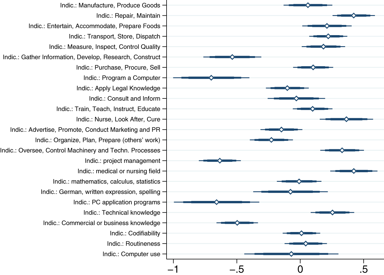
WFH and workplace characteristics.
Source: BIBB-BAuA (2018).
Notes: The figure shows the prediction from a logistic regression at the individual level. The dependent variable WFH is an indicator variable equal to one if the respondent reports to work (occasionally) from home. Indicators for workplace characteristics are described in Section 3. The number of observations is n = 17,827 and the Pseudo R-squared is 0.2419. Thick, medium, and thin lines represent the 99, 95, and 90 percent confidence intervals.
No-WFH and workplace characteristics.
Source: BIBB-BAuA (2018).
Notes: The figure shows the prediction from a logistic regression at the individual level. The dependent variable No-WFH is an indicator variable equal to one if the job cannot be performed from home. Indicators for workplace characteristics are described in Section 3. The number of observations is n = 11,351 and the Pseudo R-squared is 0.1546. Thick, medium, and thin lines represent the 99, 95, and 90 percent confidence intervals.
A.3 Robustness Regressions on Wage Premium
Working from home and wage income (alternative wage definition).
| Dependent variable: log gross hourly wage as in Spitz-Oener (2008) | |||||||
|---|---|---|---|---|---|---|---|
| PANEL A | (1) | (2) | (3) | (4) | (5) | (6) | (7) |
| WFH | 0.396*** | 0.241*** | 0.221*** | 0.214*** | 0.171*** | 0.131*** | 0.111*** |
| (0.00736) | (0.00699) | (0.00711) | (0.00701) | (0.00707) | (0.00712) | (0.00716) | |
| Observations | 15,530 | 15,530 | 15,530 | 15,530 | 15,530 | 15,530 | 15,530 |
| R-squared | 0.157 | 0.372 | 0.409 | 0.430 | 0.483 | 0.508 | 0.518 |
| PANEL B | (1) | (2) | (3) | (4) | (5) | (6) | (7) |
| log WFH hours | 0.0821*** | 0.0473*** | 0.0450*** | 0.0447*** | 0.0295*** | 0.0254*** | 0.0250*** |
| (0.00705) | (0.00616) | (0.00627) | (0.00623) | (0.00634) | (0.00625) | (0.00619) | |
| Observations | 4010 | 4010 | 4010 | 4010 | 4010 | 4010 | 4010 |
| R-squared | 0.033 | 0.292 | 0.335 | 0.355 | 0.429 | 0.453 | 0.466 |
| PANEL C | (1) | (2) | (3) | (4) | (5) | (6) | (7) |
| No-WFH | −0.157*** | −0.103*** | −0.0771*** | −0.0720*** | −0.0433*** | −0.0230*** | −0.0128 |
| (0.00862) | (0.00786) | (0.00792) | (0.00780) | (0.00807) | (0.00796) | (0.00793) | |
| Observations | 9720 | 9720 | 9720 | 9720 | 9720 | 9720 | 9720 |
| R-squared | 0.033 | 0.252 | 0.308 | 0.338 | 0.401 | 0.432 | 0.445 |
| Worker and firm controls | No | Yes | Yes | Yes | Yes | Yes | Yes |
| Industry fixed effects | No | No | Yes | Yes | Yes | Yes | Yes |
| Region fixed effects | No | No | No | Yes | Yes | Yes | Yes |
| Occupation fixed effects | No | No | No | No | Yes | Yes | Yes |
| Activity controls | No | No | No | No | No | Yes | Yes |
| Performance and skill controls | No | No | No | No | No | No | Yes |
The dependent variable in all columns and panels is the log hourly gross wage, following the definition in Spitz-Oener (2008). In Panel A, WFH is an indicator variable equal to one if the respondent reports to work (occasionally) from home. In Panel B, WFH hours denotes the number of hours working from home (in logs). In Panel C, No-WFH is an indicator variable equal to one if the job cannot be performed from home. Worker and firm controls include education (in years of schooling), indicator variables for gender, married, migrant, age-squared, experience (-squared, -cubic, and quartic), and plant-size indicators. Industry fixed effects are based on NACE 1.1. Region fixed effects are based on NUTS2. Occupation fixed effect are based on KldB-2010 classification. Activity controls include 15 different activities following the definition in Becker and Muendler (2015). Performance and skill controls include indicators for routineness, codifiability, eight different skill requirements, and an indicator for computer use. For details on the variable definitions see Section 3.
Working from home and wage income (restrictive WFH measures).
| Dependent variable: log gross hourly wage | |||||||
|---|---|---|---|---|---|---|---|
| PANEL A | (1) | (2) | (3) | (4) | (5) | (6) | (7) |
| WFHr | 0.346*** | 0.193*** | 0.173*** | 0.163*** | 0.133*** | 0.100*** | 0.0823*** |
| (0.00805) | (0.00730) | (0.00733) | (0.00721) | (0.00714) | (0.00704) | (0.00704) | |
| Observations | 14,620 | 14,620 | 14,620 | 14,620 | 14,620 | 14,620 | 14,620 |
| R-squared | 0.112 | 0.363 | 0.402 | 0.427 | 0.486 | 0.517 | 0.529 |
| PANEL B | (1) | (2) | (3) | (4) | (5) | (6) | (7) |
| log WFHr hours | 0.0688*** | 0.0378*** | 0.0360*** | 0.0350*** | 0.0239*** | 0.0198*** | 0.0201*** |
| (0.00764) | (0.00668) | (0.00681) | (0.00678) | (0.00692) | (0.00681) | (0.00674) | |
| Observations | 3035 | 3035 | 3035 | 3035 | 3035 | 3035 | 3035 |
| R-squared | 0.026 | 0.282 | 0.323 | 0.348 | 0.428 | 0.454 | 0.469 |
| Worker and firm controls | No | Yes | Yes | Yes | Yes | Yes | Yes |
| Industry fixed effects | No | No | Yes | Yes | Yes | Yes | Yes |
| Region fixed effects | No | No | No | Yes | Yes | Yes | Yes |
| Occupation fixed effects | No | No | No | No | Yes | Yes | Yes |
| Activity controls | No | No | No | No | No | Yes | Yes |
| Performance and skill controls | No | No | No | No | No | No | Yes |
The dependent variable in all columns and panels is the log hourly gross wage. In Panel A, WFHr is an indicator variable equal to one if the respondent reports to work (occasionally) from home and hours worked at home are fully or partially counted as working time. In Panel B, WFHr hours denotes the number of hours worked at home and are fully or partially counted as working (in logs). Worker and firm controls include education (in years of schooling), indicator variables for gender, married, migrant, age-squared, experience (-squared, -cubic, and quartic), and plant-size indicators. Industry fixed effects are based on NACE 1.1. Region fixed effects are based on NUTS2. Occupation fixed effect are based on KldB-2010 classification. Activity controls include 15 different activities following the definition in Becker and Muendler (2015). Performance and skill controls include indicators for routineness, codifiability, eight different skill requirements, and an indicator for computer use. For details on the variable definitions see Section 3.
Working from home and wage income (only full-time workers).
| Dependent variable: log gross hourly wage | |||||||
|---|---|---|---|---|---|---|---|
| PANEL A | (1) | (2) | (3) | (4) | (5) | (6) | (7) |
| WFH | 0.392*** | 0.241*** | 0.226*** | 0.217*** | 0.176*** | 0.139*** | 0.119*** |
| (0.00700) | (0.00657) | (0.00668) | (0.00654) | (0.00656) | (0.00659) | (0.00663) | |
| Observations | 13,680 | 13,680 | 13,680 | 13,680 | 13,680 | 13,680 | 13,680 |
| R-squared | 0.186 | 0.409 | 0.446 | 0.473 | 0.528 | 0.553 | 0.563 |
| PANEL B | (1) | (2) | (3) | (4) | (5) | (6) | (7) |
| log WFH hours | 0.0715*** | 0.0414*** | 0.0401*** | 0.0394*** | 0.0291*** | 0.0259*** | 0.0254*** |
| (0.00670) | (0.00580) | (0.00588) | (0.00582) | (0.00590) | (0.00580) | (0.00575) | |
| Observations | 3625 | 3625 | 3625 | 3625 | 3625 | 3625 | 3625 |
| R-squared | 0.030 | 0.302 | 0.357 | 0.384 | 0.453 | 0.479 | 0.491 |
| PANEL C | (1) | (2) | (3) | (4) | (5) | (6) | (7) |
| No-WFH | −0.155*** | −0.0964*** | −0.0755*** | −0.0679*** | −0.0407*** | −0.0203*** | −0.0110 |
| (0.00822) | (0.00742) | (0.00744) | (0.00725) | (0.00742) | (0.00730) | (0.00726) | |
| Observations | 8478 | 8478 | 8478 | 8478 | 8478 | 8478 | 8478 |
| R-squared | 0.040 | 0.282 | 0.340 | 0.382 | 0.451 | 0.484 | 0.498 |
| Worker and firm controls | No | Yes | Yes | Yes | Yes | Yes | Yes |
| Industry fixed effects | No | No | Yes | Yes | Yes | Yes | Yes |
| Region fixed effects | No | No | No | Yes | Yes | Yes | Yes |
| Occupation fixed effects | No | No | No | No | Yes | Yes | Yes |
| Activity controls | No | No | No | No | No | Yes | Yes |
| Performance and skill controls | No | No | No | No | No | No | Yes |
The dependent variable in all columns and panels is the log hourly gross wage. In Panel A, WFH is an indicator variable equal to one if the respondent reports to work (occasionally) from home. In Panel B, WFH hours denotes the number of hours working from home (in logs). In Panel C, No-WFH is an indicator variable equal to one if the job cannot be performed from home. Worker and firm controls include education (in years of schooling), indicator variables for gender, married, migrant, age-squared, experience (-squared, -cubic, and quartic), and plant-size indicators. Industry fixed effects are based on NACE 1.1. Region fixed effects are based on NUTS2. Occupation fixed effect are based on KldB-2010 classification. Activity controls include 15 different activities following the definition in Becker and Muendler (2015). Performance and skill controls include indicators for routineness, codifiability, eight different skill requirements, and an indicator for computer use. For details on the variable definitions see Section 3. The sample is restricted to full-time workers, i.e. workers reporting to work at least 21 h per week.
Working from home and wage income (quantile regressions).
| Dependent variable: log gross hourly wage | ||
|---|---|---|
| (1) WFH | (2) No-WFH | |
| 0.1 | 0.0927*** | −0.0320** |
| (0.0119) | (0.0144) | |
| 0.2 | 0.0920*** | −0.0160* |
| (0.00827) | (0.00967) | |
| 0.3 | 0.0945*** | −0.0222** |
| (0.00790) | (0.00890) | |
| 0.4 | 0.0969*** | −0.0250*** |
| (0.00720) | (0.00801) | |
| 0.5 | 0.0999*** | −0.0211** |
| (0.00735) | (0.00833) | |
| 0.6 | 0.104*** | −0.0163** |
| (0.00750) | (0.00772) | |
| 0.7 | 0.120*** | −0.0124 |
| (0.00776) | (0.00797) | |
| 0.8 | 0.122*** | −0.0122 |
| (0.00765) | (0.00807) | |
| 0.9 | 0.136*** | −0.0145 |
| (0.0104) | (0.0115) | |
| OLS | 0.112*** | −0.0150** |
| (0.00665) | (0.00726) | |
| Worker and firm controls | Yes | Yes |
| Industry fixed effects | Yes | Yes |
| Region fixed effects | Yes | Yes |
| Occupation fixed effects | Yes | Yes |
| Activity controls | Yes | Yes |
| Performance and skill controls | Yes | Yes |
The table shows estimates from a quantile regressions on WFH (column 1) and No-WFH (column 2) across the wage distribution (namely the quantiles 0.1, 0.2, … , 0.9), and the respective OLS estimates corresponding to the last column from Table 3. The dependent variable in all columns is the log hourly gross wage. In column 1, WFH is an indicator variable equal to one if the respondent reports to work (occasionally) from home. In column 2, No-WFH is an indicator variable equal to one if the job cannot be performed from home. Worker and firm controls include education (in years of schooling), indicator variables for gender, married, migrant, age-squared, experience (-squared, -cubic, and quartic), and plant-size indicators. Industry fixed effects are based on NACE 1.1. Region fixed effects are based on NUTS2. Occupation fixed effect are based on KldB-2010 classification. Activity controls include 15 different activities following the definition in Becker and Muendler (2015). Performance and skill controls include indicators for routineness, codifiability, eight different skill requirements, and an indicator for computer use. For details on the variable definitions see Section 3. The regressions in column 1 and 2 are based on 15,530 and 9720 observations, respectively.
Working from home and wage income (detailed regression output).
| Dependent variable: log gross hourly wage | |||
|---|---|---|---|
| WFH | 0.112*** | ||
| (0.00665) | |||
| log WFH hours | 0.0233*** | ||
| (0.00587) | |||
| No-WFH | −0.0150** | ||
| (0.00726) | |||
| Education | 0.0242*** | 0.0342*** | 0.0236*** |
| (0.00522) | (0.0121) | (0.00668) | |
| Indic.: Female | −0.119*** | −0.123*** | −0.0996*** |
| (0.00642) | (0.0130) | (0.00809) | |
| Indic.: Married | 0.0431*** | 0.0499*** | 0.0429*** |
| (0.00539) | (0.0117) | (0.00647) | |
| Age2 | 0.00862 | 0.00162 | 0.00496 |
| (0.00529) | (0.0123) | (0.00684) | |
| Experience | 0.0252*** | 0.0323* | 0.0303*** |
| (0.00784) | (0.0173) | (0.00957) | |
| Experience2 | −0.0964* | −0.116 | −0.135** |
| (0.0517) | (0.115) | (0.0620) | |
| Experience3 | 0.142 | 0.235 | 0.272 |
| (0.144) | (0.331) | (0.173) | |
| Experience4 | −0.0884 | −0.199 | −0.214 |
| (0.139) | (0.328) | (0.165) | |
| Indic.: Migrant | −0.0227** | −0.0329 | −0.0256** |
| (0.0101) | (0.0227) | (0.0119) | |
| Observations | 15,530 | 4010 | 9720 |
| R-squared | 0.537 | 0.476 | 0.466 |
| Worker and firm controls | Yes | Yes | Yes |
| Industry fixed effects | Yes | Yes | Yes |
| Region fixed effects | Yes | Yes | Yes |
| Occupation fixed effects | Yes | Yes | Yes |
| Activity controls | Yes | Yes | Yes |
| Performance and skill controls | Yes | Yes | Yes |
The dependent variable in all columns is the log hourly gross wage and the regressions are akin to the last column from Table 3 for Panel A, B, and C. In column 1, WFH is an indicator variable equal to one if the respondent reports to work (occasionally) from home. In columns 2, WFH hours denotes the number of hours working from home (in logs). In column 3, No-WFH is an indicator variable equal to one if the job cannot be performed from home. Worker and firm controls include education (in years of schooling), indicator variables for gender, married, migrant, age-squared, experience (-squared, -cubic, and quartic), and plant-size indicators. Industry fixed effects are based on NACE 1.1. Region fixed effects are based on NUTS2. Occupation fixed effect are based on KldB-2010 classification. Activity controls include 15 different activities following the definition in Becker and Muendler (2015). Performance and skill controls include indicators for routineness, codifiability, eight different skill requirements, and an indicator for computer use. For details on the variable definitions see Section 3. Note that regression output for age is dropped as it is controlled for via the variables experience and education, as experience is defined as age-education-5.
A.4 Further Results on Regional Analysis

Working from home and wages across federal states in Germany.
Source: BIBB-BAuA 2018 (projection factor based on microcensus 2017).
Notes: The upper left panel depicts the average of WFH and the average log hourly wage for the 16 federal states in Germany. The upper right panel uses the average log residual wage after running a mincer regression (see Section 4.2 for details). The lower left (right) panel depicts the average of No-WFH and the average log hourly wage (average log residual wage).

Working from home and wages in Germany (alternative WFH measure).
Source: BIBB-BAuA 2018 (projection factor based on microcensus 2017) and Fadinger and Schymik (2020).
Notes: The figure depicts the working from home potential from Fadinger and Schymik (2020) and the average log hourly wage (from the BIBB-BAUA 2018 sample) for 38 different NUTS2 regions in Germany.
Summary statistics for NUTS2 regions in Germany.
| NUTS2 | NUTS2 Name | WFH | No-WFH | Wage | Residual wage | N(WFH) | N(No-WFH) |
|---|---|---|---|---|---|---|---|
| DEF0 | Schleswig-Holstein | 0.24 | 0.46 | 2.87 | 0.02 | 610 | 411 |
| DE60 | Hamburg | 0.36 | 0.35 | 2.92 | 0.01 | 469 | 271 |
| DE91 | Statistical region Brunswick | 0.23 | 0.48 | 2.91 | −0.02 | 328 | 219 |
| DE92 | Statistical region Hanover | 0.25 | 0.46 | 2.91 | 0 | 476 | 309 |
| DE93 | Statistical region Lueneburg | 0.29 | 0.44 | 2.82 | −0.01 | 356 | 222 |
| DE94 | Statistical region Weser-Ems | 0.2 | 0.5 | 2.8 | −0.02 | 502 | 350 |
| DE50 | Bremen | 0.23 | 0.49 | 2.83 | −0.03 | 145 | 87 |
| DEA1 | Duesseldorf | 0.28 | 0.4 | 2.96 | 0.03 | 852 | 522 |
| DEA2 | Cologne | 0.35 | 0.4 | 2.96 | 0 | 808 | 432 |
| DEA3 | Muenster | 0.29 | 0.42 | 2.92 | 0.02 | 434 | 280 |
| DEA4 | Detmold | 0.23 | 0.48 | 2.85 | 0.02 | 459 | 306 |
| DEA5 | Arnsberg | 0.27 | 0.45 | 2.9 | 0.03 | 674 | 428 |
| DE71 | Darmstadt | 0.38 | 0.34 | 2.98 | 0.02 | 843 | 464 |
| DE72 | Giessen | 0.3 | 0.39 | 2.86 | −0.07 | 195 | 120 |
| DE73 | Kassel | 0.21 | 0.54 | 2.88 | −0.01 | 230 | 158 |
| DEB1 | Statistical region Koblenz | 0.31 | 0.43 | 2.93 | −0.01 | 269 | 165 |
| DEB2 | Statistical region Trier | 0.31 | 0.45 | 2.88 | 0 | 97 | 59 |
| DEB3 | Statistical region Rhine-Hesse-Palatinate | 0.31 | 0.35 | 2.94 | 0.01 | 396 | 240 |
| DE11 | Stuttgart | 0.29 | 0.37 | 2.96 | 0.03 | 778 | 469 |
| DE12 | Karlsruhe | 0.3 | 0.39 | 3.01 | 0.05 | 580 | 342 |
| DE13 | Freiburg | 0.21 | 0.46 | 2.92 | 0.08 | 418 | 290 |
| DE14 | Tuebingen | 0.27 | 0.43 | 2.91 | 0.07 | 360 | 218 |
| DE21 | Upper Bavaria | 0.35 | 0.38 | 2.95 | 0.07 | 1419 | 828 |
| DE22 | Lower Bavaria | 0.23 | 0.48 | 2.92 | 0.07 | 308 | 207 |
| DE23 | Upper Palatinate | 0.24 | 0.54 | 2.89 | 0.03 | 309 | 204 |
| DE24 | Upper Franconia | 0.28 | 0.47 | 2.88 | −0.01 | 276 | 183 |
| DE25 | Middle Franconia | 0.24 | 0.43 | 2.93 | 0.02 | 507 | 323 |
| DE26 | Lower Franconia | 0.19 | 0.44 | 2.78 | −0.08 | 342 | 243 |
| DE27 | Swabia | 0.19 | 0.52 | 2.85 | 0.06 | 495 | 344 |
| DEC0 | Saarland | 0.26 | 0.38 | 2.93 | 0.03 | 187 | 124 |
| DE30 | Berlin | 0.36 | 0.33 | 2.89 | −0.05 | 1029 | 617 |
| DE40 | Brandenburg | 0.24 | 0.47 | 2.8 | −0.08 | 528 | 378 |
| DE80 | Mecklenburg-Western Pomerania | 0.22 | 0.56 | 2.72 | −0.09 | 328 | 229 |
| DED4 | Directorate region Chemnitz | 0.17 | 0.58 | 2.65 | −0.18 | 285 | 224 |
| DED2 | Directorate region Dresden | 0.23 | 0.51 | 2.74 | −0.11 | 375 | 261 |
| DED5 | Directorate region Leipzig | 0.28 | 0.43 | 2.79 | −0.12 | 240 | 158 |
| DEE0 | Saxony-Anhalt | 0.21 | 0.48 | 2.66 | −0.17 | 455 | 334 |
| DEG0 | Thuringia | 0.21 | 0.53 | 2.71 | −0.13 | 465 | 332 |
The table reports averages for WFH (an indicator variable equal to one if the respondent reports to work from home), No-WFH (an indicator variable equal to one if the job cannot be performed from home), log gross hourly wages, residual wages after running a Mincer regression (see Sections 4.2 for details), and the number of underlying observations – N(WFH) and N(No-WFH) – for the 38 different NUTS2 regions in Germany.
BIBB-BAuA 2018 (projection factor based on microcensus 2017).
References
Acemoglu, D. and Pischke, J.-S. (1998). Why do firms train? Theory and evidence. Q. J. Econ. 113: 79–119, https://doi.org/10.1162/003355398555531.Search in Google Scholar
Adams-Prassl, A., Boneva, T., Golin, M., and Rauh, C. (2020). Inequality in the impact of the coronavirus shock: evidence from real time surveys. J. Publ. Econ. 189: 104245, https://doi.org/10.1016/j.jpubeco.2020.104245.Search in Google Scholar
Alipour, J.-V., Fadinger, H., and Jan, S. (2020a). My home is my castle–the benefits of working from home during a pandemic crisis: evidence from Germany, Technical Report, CEPR Discussion Papers.10.1016/j.jpubeco.2021.104373Search in Google Scholar
Alipour, J.-V. , Falck, O., and Schüller, S. (2020b). Germany’s capacities to work from home. Technical Report, CESifo Working Paper.10.2139/ssrn.3579244Search in Google Scholar
Alipour, J.-V., Falck, O., and Schüller, S. (2020c). Homeoffice während der Pandemie und die Implikationen für eine Zeit nach der Krise. Ifo Schnelld. 73: 30–36.Search in Google Scholar
Autor, D., Dorn, D., and Hanson, G.H. (2013). The China syndrome: local labor market effects of import competition in the United States. Am. Econ. Rev. 103: 2121–2168, https://doi.org/10.1257/aer.103.6.2121.Search in Google Scholar
Barbieri, T., Basso, G., and Scicchitano, S. (2020). Italian workers at risk during the Covid-19 epidemic. Available at SSRN 3572065.10.2139/ssrn.3660014Search in Google Scholar
Becker, S.O. and Muendler, M.A. (2015). Trade and tasks: an exploration over three decades in Germany. Econ. Pol. 30: 589–641, https://doi.org/10.1093/epolic/eiv014.Search in Google Scholar
Bloom, N., Liang, J., Roberts, J., and Ying, Z.J. (2015). Does working from home work? Evidence from a Chinese experiment. Q. J. Econ. 130: 165–218, https://doi.org/10.1093/qje/qju032.Search in Google Scholar
Brynjolfsson, E., Horton, .J.J., Adam, O., Rock, D., Sharma, G., and TuYe, H.-Y. (2020). COVID-19 and remote work: an early look at US data. Working Paper 27344, National Bureau of Economic Research.10.3386/w27344Search in Google Scholar
Card, D., Heininge, J., and Kline, P. (2013). Workplace heterogeneity and the rise of West German wage inequality. Q. J. Econ. 128: 967–1015, https://doi.org/10.1093/qje/qjt006.Search in Google Scholar
Dauth, W., Findeisen, S., Moretti, E., and Suedekum, J. (2018). Matching in cities. Technical Report, National Bureau of Economic Research.10.3386/w25227Search in Google Scholar
DiNardo, J.E. and Pischke, J.S. (1997). The returns to computer use revisited: have pencils changed the wage structure too? Q. J. Econ. 112: 291–303, https://doi.org/10.1162/003355397555190.Search in Google Scholar
Dingel, J.I. and Neiman, B. (2020). How many jobs can be done at home? J. Publ. Econ. 189: 104235, https://doi.org/10.1016/j.jpubeco.2020.104235.Search in Google Scholar
Fadinger, H. and Schymik, J. (2020). The costs and benefits of home office during the Covid-19 pandemic: evidence from infections and an input-output model for Germany. COVID Econ.: Vetted and Real-Time Pap. 9: 107–134.Search in Google Scholar
Gathmann, C. and Schönberg, U. (2010). How general is human capital? A task-based approach. J. Labor Econ. 28: 1–49, https://doi.org/10.1086/649786.Search in Google Scholar
Gottlieb, C., Grobovšek, J., and Poschke, M. (2020). Working from home across countries. Covid Econ. 1: 71–91.10.2139/ssrn.3699854Search in Google Scholar
Heise, S. and Porzio, T. (2019). Spatial wage gaps and frictional labor markets. Technical Report 898.10.2139/ssrn.3467682Search in Google Scholar
Kondo, K. (2018). Testing for global spatial autocorrelation in Stata. Available at: http://fmwww.bc.edu/RePEc/bocode/m/moransi.pdf.Search in Google Scholar
Mergener, A. (2020). Occupational access to the home office: a task-based approach to explaining unequal opportunities in home office access. Kölner Z. Soziol. Sozialpsychol.: 1–24. https://doi.org/10.1007/s11577-020-00669-0.Search in Google Scholar
Mongey, S. and Weinberg, A. (2020). Characteristics of workers in low work-from-home and high personal-proximity occupations, Working Paper, Becker Friedman Institute.Search in Google Scholar
Moretti, E. (2011). Local labor markets. In: Handbook of labor economics, Vol. 4. Elsevier, Amsterdam, North-Holland, pp. 1237–1313.10.3386/w15947Search in Google Scholar
Palomino, J.C., Rodríguez, J.G., and Sebastian, R. (2020). Wage inequality and poverty effects of lockdown and social distancing in Europe. Covid Econ.: 186. https://doi.org/10.1016/j.euroecorev.2020.103564.Search in Google Scholar
Saltiel, F. (2020). Who can work from home in developing countries. Covid Econ. 7: 104–118.Search in Google Scholar
Shapiro, C. and Stiglitz, J.E. (1984). Equilibrium unemployment as a worker discipline device. Am. Econ. Rev. 74: 433–444.10.1017/CBO9780511559594.004Search in Google Scholar
Spitz-Oener, A. (2006). Technical change, job tasks, and rising educational demands: looking outside the wage structure. J. Labor Econ. 24: 235–270.10.1086/499972Search in Google Scholar
Spitz-Oener, A. (2008). The returns to pencil use revisited. Ind. Labor Relat. Rev. 61: 502–517, https://doi.org/10.1177/001979390806100404.Search in Google Scholar
von Gaudecker, H.-M., Holler, R., Janys, L., Siflinger, B.M., and Zimpelmann, C. (2020). Labour supply during lockdown and a new normal: the case of the Netherlands, IZA Discussion Paper 13623. Bonn, Institute of Labor Economics (IZA).10.2139/ssrn.3682937Search in Google Scholar
© 2020 Walter de Gruyter GmbH, Berlin/Boston
Articles in the same Issue
- Frontmatter
- Original Articles
- COVID-19 and Financial Markets: A Panel Analysis for European Countries
- French Firms and COVID-19: Do the Debt Status, Crisis Management System, and Monetary Policy Play a Role?
- Working from Home, Wages, and Regional Inequality in the Light of COVID-19
- Data Observer
- Green-SÖP: The Socio-ecological Panel Survey: 2012–2016
- Book Review
- Aufderheide, Detlef und Martin Dabrowski: Digitalisierung und Künstliche Intelligenz. Wirtschaftsethische und moralökonomische Perspektiven