Recursive Gauss-Helmert model with equality constraints applied to the efficient system calibration of a 3D laser scanner

2.1 Gauss-Helmert model

In general, the use of a suitable estimator is required to perform parameter estimation. In the context of batch processing, least-squares can be applied. For this estimator the optimisation criterion is to minimize the sum of the squared residuals v between real observations l and their corresponding expected values E l , which are functions of the unknown parameters x [32]. This method is referred to as least-squares adjustment and is widely used in the geodetic community where it is well described by [28], [32], [35], [39], [66].

The residuals v are assumed to be Gaussian with expected value E v = 0

where Σ l l is the known variance-covariance matrix (VCM) of the observations, Q l l the related cofactor matrix, σ 0 2 the a priori variance factor and P the weight matrix. Together, these parameters describe the weighting of the observations among themselves and are referred to as a stochastic model. In the context of this contribution, a simplified stochastic model with independent and identically distributed random variables is assumed for the application in section 4.

Since the adjustment approach requires linear functional models, Taylor series expansion is performed to linearise h · . In the context of linearisation and subsequent optimisation, this is an iterative process in which the individual variables must be updated in each iteration step. Suitable approximate values of l 0 and x 0 for both the observations E l and the unknown parameters x are needed for the first epoch [35]. Their reasonable selection has a direct impact on the number of required repetitions as well as on the successful convergence to the global optimum. For the sake of clarity, detailed information on the individual iterations is not given here, but readers are referred to the detailed descriptions in previous works (e. g. [32], [33], [35]). Specifying the theoretical quantities, the following applies

where B is the condition matrix with partial derivatives with respect to the observations, A is the design matrix with partial derivatives with respect to the parameters, Δ x is the reduced parameter vector and w refers to the contradictions according to

Using the utility matrix Q b b

the solution of the objective function L GHM v , Δ x , λ leads to the linear normal equation system in block structure, when setting the related partial derivatives equal to zero

Here N GHM is referred to as the normal equation matrix, which must be regular to be invertible.

The estimate of the requested parameter vector x ˆ can be obtained by the inverse of the normal equation matrix N GHM , considering the relationship to the reduced parameter vector Δ x as follows

The residuals v ˆ result from the estimated observations l ˆ as follows

As this is an iterative process, the approximate values l 0 and x 0 are subsequently updated by the current estimated values.

2.2 Gauss-Helmert model with equality constraints

If reliable and suitable prior knowledge about the parameters is available, it is always advisable to integrate this additional information into the estimation process [4], [47], [51]. Any mathematical definitions, physical laws, geometric constraints or other practical or logical specifications can be taken into account. An extension of the GHM by equality constraints (referred to as constrained GHM (C-GHM)) is therefore introduced in [22], [36], [44], [46], [55] according to

where D is the matrix of equality constraints and d is the related constant vector. In general, however, such constraints are described by non-linear relationships

which must be linearised by a first-order Taylor expansion to obtain Equation (18) according to

In order to find the minimum of the objective function L C-GHM v , Δ x , λ 1 , λ 2 , the partial derivatives must be set to zero

The cofactor matrix Q x ˆ x ˆ can be derived by

with the regular auxiliary matrix

The estimated residuals v ˆ can be obtained by substitution and transformation of Equation (5) and Equation (24) as follows

According to [22], the aforementioned substitution can be used to reduce the normal equation system by eliminating the Lagrange multiplier

which means that λ ˆ 1 can be substituted in Equation (25) leading to

Using this substitution the simplified normal equation system consists of the following

Even though the normal equation system has already been set up in Equation (28) and contains the solution for the requested parameters, the advantage of Equation (34) is that it is less dimensional, which can have a positive effect on the run time with regard to big data. Furthermore, the application to the data set presented in section 4 has indicated that in individual cases the solution via Equation (34) is numerically more stable and therefore more reliable depending on the geometric configuration. This relates directly to the number of constraints to be considered, which affects the condition of the normal equation matrix due to multiple zero elements. Again, several iterations for repeated linearisation are required to obtain the parameters requested by the inverse of the normal equation matrix N C-GHM ∗ .

3.1 Recursive state-space filtering

In contrast to parameter estimation, recursive state-space filtering uses additional system information besides the measurement information. This makes it possible to consider suitable physical models that mathematically describe the temporal and spatial dynamics of the requested state parameters. Thus, both measurements and physical properties are considered. In general, an IEKF is an advancement of the linear Kalman filter (KF) and enables the possibility to consider non-linear relationships [7]. Both are applied by means of a recursive two-step procedure for state estimation over a theoretically unlimited amount of epochs. Arbitrary types of state parameters x k (e. g., position, orientation, velocity) are forecasted by a suitable process model f ( · ) during the prediction step and corrected by latest sensor measurements subsequently within each epoch k. Selected physical relationships (e. g. motion models) are applied to the previous state parameters x k − 1 from the last past epoch. Further affecting influencing factors like zero-mean process noise w k with VCM Σ w w , k and controls u k are also applied. According to [50], the non-linear process model is given by

During the update step, the predicted state parameters are corrected using the latest sensor observations l k using the non-linear measurement equations h ( · ). In most approaches, only explicit relationships (cf. Equation (1)) can be applied. However, the IEKF from [5], [6] enables application of implicit relations between observations and states

To distinguish between the predicted and updated state parameters, x k − is referred to the a priori estimate and x k + to the a posteriori estimate of the state vector. The corresponding VCM for the predicted state is given by Σ x x , k − and for the updated state by Σ x x , k + .

Consideration of this implicit measurement equation during the update step is done by the objective function L IEKF according to [5], [6] as follows

where l k + are the updated observations and both A k and B k are the Jacobian matrices with respect to the states and the observations

where

Figure 1

Flowchart of the versatile recursive state-space filter based on an IEKF for non-linear implicit and explicit measurement equations with predicted states (solid box) and updated states & observations (dotted box) according to [64].

The filtered observations and states can be obtained by the inverse of the normal equation matrix N IEKF , similar to the solution of GHM in the batch processing approach. In contrast to an extended Kalman Filter (EKF), which can also handle non-linear relations, the IEKF comprises repeated iteration runs for m = 0 … M − 1 during the update step within each epoch k. This reduces the impact of the non-linearities. This is comparable to the GHM in batch processing (cf. section 2). In each epoch k, the development points x ˇ k , m and l ˇ k , m are initialized by

In this context, it should also be mentioned that there are also corresponding uncertainty information in the form of the VCM Σ l ˆ l ˆ , k + in addition to the filtered observations l ˆ k + .

Algorithm 1

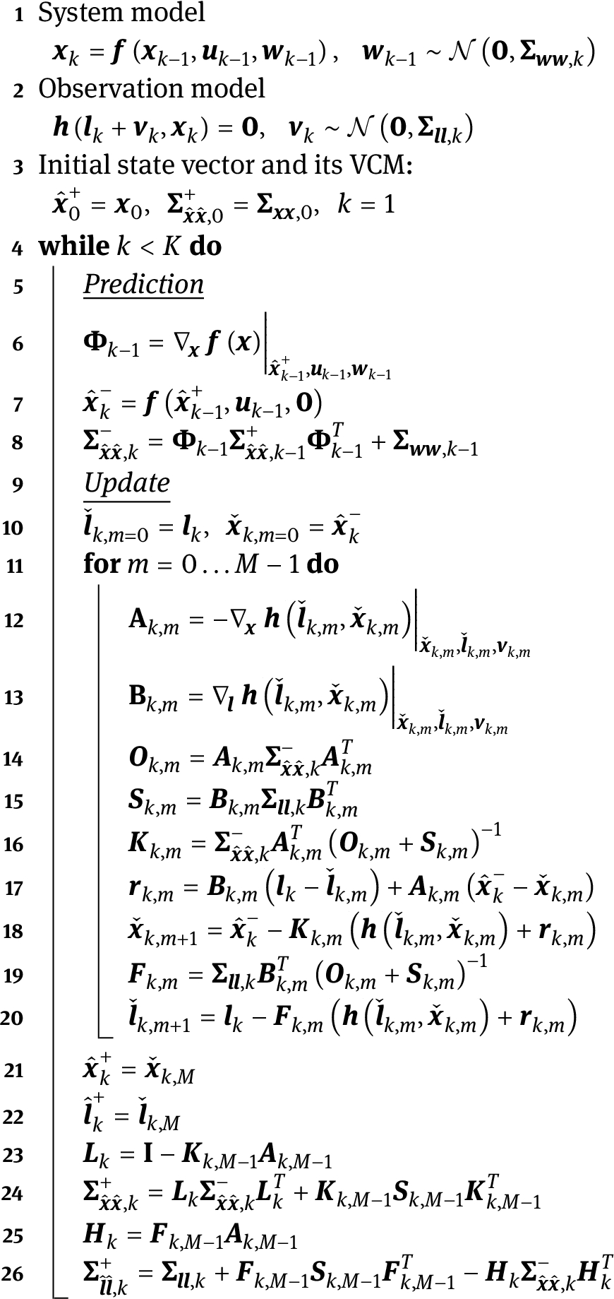
Versatile recursive state-space filter based on an IEKF for non-linear implicit and explicit measurement equations.

3.2 Recursive Gauss-Helmert model

The IEKF, described in Algorithm 1, is open towards different physical motion and measurement models. In contrast to the vast majority of existing IEKF realisations, both implicit and explicit relations can be applied (cf. Equation (3)). This is a crucial advantage and allows more flexibility regarding new applications. Furthermore, a recursive GHM can be introduced on the basis of this IEKF, which did not exist before. This new method was first introduced in [64] and enables the possibility to receive state estimates on an epoch-wise basis. As already motivated in section 1, such a recursive approach is particularly suitable for more efficient processing of big data. The main difference between the recursive parameter estimation and the recursive state estimation is the consideration of a dynamic model within the prediction step (cf. Equation (35)), if a filter approach is used.

Therefore, to realise such a recursive GHM, the prediction step and related system model of the IEKF are disregarded. In this case, the predicted state x k − (cf. line 7 in Algorithm 1) is identical to the filtered state x k − 1 + from the last past epoch. The same applies for the related VCM Σ x x , k − (cf. line 8 in Algorithm 1), whereby a suitable process noise Σ w w , k can still be considered. Suitable in this context means that numerical instabilities are avoided, but no excessive influence results from its choice. In theory, the process noise should be zero for a recursive GHM. Since the realisation here is based on an IEKF, which requires a sufficiently accurate initialisation, the consideration of a non-zero process noise has a regularising effect. This behaviour could be identified within the framework of numerical investigations but will be analysed in more detail in the future. It has been shown that the total disregard of the system noise has had a particularly negative effect on the estimation results of the first epochs, as these have been given too much weight. Thus, the approximate values for the subsequent epochs were also influenced, and the adjustment diverged in some cases. The respective order of magnitude and physical interpretation should be considered depending on the specific application. In each case, it is also important to investigate the extent to which the additional information in the stochastic model could lead to a possible bias in the estimate. Since taking system noise into account influences the weighting in the update step between the predicted and observed quantities, too strong input can lead to inaccurate results. In particular, comprehensive sensitivity analyses are recommended for this purpose. Further investigations on this can be found in [64]. The following applies for the prediction step of the recursive GHM

3.3 Recursive Gauss-Helmert model with equality constraints

Consideration of suitable state constraints for arbitrary linear and non-linear KF approaches with explicit measurement equation are well-practised [18], [50], [51]. However, the combination of Kalman filtering with implicit measurement equations and state constraints is almost non-existing. A first approach is given by [62], where non-linear equality constraints are considered by means of a projection method. An extension regarding non-linear inequality state constraints using probability density function (PDF) truncation is given in [63]. However, both projection and PDF truncation in terms of implicit relations will lead to unfulfilled contradictions. This issue is stated in [63] and occurs due to the subsequent constraint step between the update and prediction step. Only the states are affected during the constraint step for the projection or PDF truncation method, while observations remain unaffected. For this reason, we present two methods for consideration of equality constraints, which overcome this issue and were initially introduced in [64]. As these state constraints can be applied by the IEKF for implicit measurement equation, introduced at the beginning of section 3, they are also applicable for the recursive GHM (cf. section 3.2). This will be referred to as recursive C-GHM with reference to the respective constraint method.

4.1 Experimental setup

For the sake of clarity, only a simplified representation of an MSS is given below. Nevertheless, the basic procedure can be transferred directly to any MSS with an LS to be calibrated. In particular, the SOCS of a Velodyne Puck VLP-16 is to be calibrated with respect to a specific PCS. The platform for mounting the LS has drilling holes that define the PCS (cf. Figure 2(a)). By using these drilling holes, the joint adaptation can be applied universally on any other platform. The spatial relationship to the SOCS of the LS can then be established via the drilling holes and the calibration parameters. The platform with the LS is shown in Figure 2 together with both PCS and SOCS. The 6-DoF calibration parameters between these two coordinate systems are thus to be determined. The used LS measures with 16 individual scan lines, which are almost perpendicular to its vertical axis and have an angular resolution of around 2 °. Combining these single scan lines and an internal rotation results in a panoramic 3D point cloud (PCL). Altogether, the LS has a field of view of 30 ° × 360 °. The manufacturer specifies a range accuracy of typically up to 3 cm [60], without indicating the associated quality parameter.

Figure 2

LS-based MSS with Velodyne Puck VLP-16 LS on a platform with numbered drilling holes (a) and schematic representation of the MSS with the red PCS and the blue SOCS of the LS (b), according to [64].

To determine the calibration parameters between the SOCS of the LS and the PCS, multiple reference planes are arranged in the field of view of the LS within the 3D-Laboratory of the Geodetic Institute of the Leibniz University Hannover. There are 12 planes in the field of view of the LS, which differ in their distance to the MSS and their respective size. A detailed description of the reference planes used regarding their spatial distribution and orientation is given in [21]. Attention must be paid to a versatile alignment of the individual planes in order to ensure high sensitivity and quality for the individual coordinate axes [21], [23]. In this context, it should be noted that only a few (but at least two) of all 16 scan lines per reference plane will capture them at all. This results from the distance and size of the reference planes. In order to obtain known nominal values for the reference planes, they must be determined and mathematically described with a sensor of superordinate accuracy. This can be done with a terrestrial LS or a total station, for example. For the investigations shown here, a highly-accurate Leica Absolute Tracker AT960 was used which, according to [25], has an maximum permissible error (MPE) of ± 15 µm + 6 µm/m for the 3D position. With its specific SOCS, the laser tracker defines a superordinate world coordinate system (WCS). Since this referencing sensor can also measure the drilling holes on the platform, an unambiguous relationship between all the coordinate systems mentioned can be realised. A part of the experimental setup, the relevant observations and related coordinate systems are shown in Figure 3.

Figure 3

Visualisation of the LS-based MSS (centre) during its calibration. The reference planes (left) are captured by individual scan lines (red dots) and measured (green dots) by the laser tracker (right). In addition, the drilling holes on the platform (yellow stars) are measured with the laser tracker (right). Due to the perspective, the PCS can only be displayed to a limited extent. Further arranged planes are located outside the shown part of the image. Modified according to [64].

A rotation speed of 10 Hz is selected for acquisition by the LS, with a total measuring time of 5 seconds. After cropping the PCL of unnecessary points of the laboratory environment and assigning the points to the reference planes, in total, between 500 and 6000 points per plane are available for the calibration. To avoid outliers in the later analysis, the assignment is done manually. The whole data set was collected in the course of the work of [13].

4.2 State-of-the-art calibration approach

As a state-of-the-art approach, the calibration procedure for LS-based MSS using reference geometries (RFG) from [56] is used, which is inspired by the work of [44] and [17]. This methodical approach states that the distances between the observed reference planes and the measured 3D point observations of the LS to be calibrated should be minimal. To describe this condition in a functional model, two similarity transformations are needed to transform the SOCS via the PCS to the WCS. Therefore all j e = 1 , … , J e sets of 3D points P LS , e , j e measured by the LS with respect to its local SOCS and assigned to the e = 1 , … , E individual reference planes need to be transformed according to

where P MSS , e , j e are the transformed LS 3D points with respect to the PCS. To establish a connection to the WCS, a further transformation is necessary

where P LT , e , j e are the transformed LS 3D points with respect to the WCS. In both equations (58) and (59), R stands for the respective 3D rotation matrix resulting from the corresponding three Euler angles. Together with the respective translations t SOCS-PCS and t PCS-WCS , this results in the requested 6-DoF transformation parameters

and

In order to estimate these parameters, the approach of [56] solves the calibration task by constraining the distances d j e within a GHM (cf. Equation (2)). The functional relationship between the observations and parameters reads

The first three elements describe the 3×1 unit normal vector n RFG , e and d RFG , e the distance to the origin. The observed quantities in this implicit relationship are arranged in the observation vector l as follows

where e = 1 , … , E. In [56], both the plane parameters a RFG , e as well as the transformation parameter t ¯ PCS-WCS are considered to be original observations. This leads to a reduced adjustment problem and is recommended due to the high information density that already occurs. The stochastic model chosen for the adjustment sets all LS observations as uncorrelated and with the same standard deviation of σ LS , 0 = 0.01 m. Thus, with respect to the observation vector from Equation (64), the VCM Σ LS , l l for the 3D LS points P LS , e , j e can be given as follows

where I LS is the identity matrix with the appropriate dimension in terms of the number of all LS observations. For the entire VCM Σ l l , uncertainty information of the 6-DoF calibration parameters t ¯ PCS-WCS as well as the plane parameters a RFG , e need to be added. This variance-covariance information can be obtained in the context of a simplified pre-adjustment and is considered as stochastic prior information by means of a fully populated VCM. Thus, a comparability to the recursive approach presented in section 4.3 can be realised.

In [19], [56], the application of this method is based on the assumption that the transformation parameters between WCS and PCS and the plane parameters themselves are error-free quantities (deterministic) that are known and constant. This is justified by using a reference sensor with superordinate accuracy in relation to the uncertainty level of the LS. However, in the context of this paper, these parameters shall be considered as stochastic quantities. This is reasonable since using a 3D Velodyne VLP-16 with multiple scan lines allows estimation of the individual reference planes. In [19], [56], this was not possible due to the respective use of a 2D profile LS. To enable a more general approach, the parameter vector here results as follows

Since the plane parameters a RFG , e are part of the parameter vector, the consideration of constraints is necessary, so that their normalized unit length can be guaranteed and geometrical or numerical instabilities do not occur. This leads to a non-linear equality constraint (cf. Equation (19)) for all e reference planes regarding the respective normal vector n RFG , e as follows

For the consideration of this additional information in the batch approach, the C-GHM from section 2.2 has to be applied.

The concatenated transformations with the inclusion of rotations bring challenges for adjustment. As already mentioned in section 2.1, suitable approximate values are required for the solution of the C-GHM to converge. These can be based on rough dimensions and can be updated after a successful adjustment, if necessary.

As a further extension to [19], [56], it can be reasonable for the quality of the calibration parameters to perform the acquisition process of the static reference geometries by the MSS from multiple different positions. In [13], it was shown that this allowed the individual transformation parameters to be decorrelated. As long as the planes are constant over time between the individual measurements, a better distribution of the measuring points on the planes could be realised. The use of multiple viewpoints may also allow certain planes that do not have geometrically sufficient coverage from a single viewpoint to be considered at all. For the adjustment approach this means that one set of 6-DoF transformation parameters between PCS and WCS (cf. Equation (61)) must be considered per calibration position s as follows

and accordingly, further measurement equations must be included. The plane parameters a RFG , e remain numerically and in number unchanged. Even if the number of individual configurations is theoretically unlimited and is advantageous, the amount of data to be taken into account is increased enormously. For the batch approach in particular, this is not practical. For this reason, this article will only deal with the combined use of two standpoints. This allows a comparison between the batch and the subsequent recursive approach, even if the latter has fewer difficulties in considering multiple viewpoints. The parameter vector from Equation (66) thus changes to

4.3 Novel recursive and constrained calibration approach

In order to obtain the 6-DoF calibration parameters given in Equations (60) and (61), a recursive estimation can be performed in addition to the batch approach from section 4.2, thus achieving a higher efficiency. However, this requires a transition to discrete epochs. For this purpose, the available LS observations of all reference planes are subdivided into k = 1 , … , K individual epochs. With regard to the experimental setup described in section 4.1, a complete 360 ° rotation of the LS is used for the definition of one single epoch k. It must be ensured that in each epoch every plane is represented by at least three to five point observations so that the recursive estimation can converge. For redundancy reasons, more observations are generally more appropriate, but this is the minimum configuration. In the specific case here, this is mainly due to the fact that only a few point observations cover the smallest reference planes, but an equal number of points per plane should be realised overall. As already mentioned in section 4.2, this can be realised by using s = 2 independent calibration positions. Thus, there are for each epoch k in total n e = 3 , … , N e 3D LS observations on each plane e, where N e can be different for each of the E = 12 planes in total and must not be constant for each epoch k. Thus the following observation vector l k results in dependence of the respective epoch k

where e = 1 , … , E. In general, both the plane parameters a RFG , k , e and the transformation parameters t ¯ PCS-WCS , k , s from the PCS to the WCS can be observed and considered in each epoch k. For practical reasons in the experimental procedure, it is also possible to proceed with a shortened observation vector l k for epochs k > 1

The basic workflow for the PCL processing is shown schematically in Figure 4. In this context, the allocation of the entire PCL (for each position s) with regard to the individual reference planes as well as the individual epochs is described.

Figure 4

Basic workflow of the PCL processing. The original PCLs are assigned to the individual reference planes, which provides the basis for the batch approach. For the recursive approach, the observations are additionally subdivided into individual epochs k.

Compared with the parameter vector in Equation (69), the estimation of the state vector x k is now also recursive for each epoch k. As already mentioned in section 4.2, parts of the observation vector are also considered in the recursive parameter vector as quantities to be estimated. Therefore, in the specific experiment here, this comprises in detail 66 states and the following applies

Furthermore, the non-linear constraint regarding the plane parameters according to equation (67) has to be considered, which is also done epoch by epoch

The techniques (namely COF and PM) described in section 3.3 are applied to account for these constraints within the recursive C-GHM. A comparison of the results among each other and in relation to the batch C-GHM follows in section 5.

The results include a comparison to another special method for considering the constraints, which was initially shown in [13]. This approach is based on a modified functional model and is not directly transferable to other application examples. Here, the idea is to supplement the functional relationship according to equation (62) by a normalisation (norm) of the plane parameters n RFG , k , e as follows

However, in general, the techniques from section 3.3 offer greater flexibility towards other applications.

Just like the C-GHM in batch processing, the recursive C-GHM also requires sufficiently accurate approximate values for the state vector x 0 to initialize. Since the recursive C-GHM is based on a IEKF, it is necessary to specify an initial VCM Σ x x , 0 for the state vector and to consider additional process noise Σ w w , k in general. The uncertainty information regarding the initial values can be provided through a simplified pre-adjustment, already mentioned in section 4.2. This information is already considered in the GHM as stochastic prior information to ensure comparability between batch and recursive adjustment. The initial values for the recursive approach thus also result from such a pre-adjustment. Their specific numerical values depend on a random selection of the point observations used. The break criterion for the iteration in both approaches is also the same. The iteration process terminates when all contradictions are smaller than 1 · 10 − 10 .

As already mentioned in section 3.2, the process noise σ w should theoretically be zero. However, investigations in [64] also indicate a regularising influence when using a suitable order of magnitude for the noise. This cannot be stated universally and depends on the respective application scenario and the corresponding influencing factors. For the recursive C-GHM here, a process noise Q w w = I · σ w , with σ w = 1 · 10 − 6 is introduced to overcome numerical instabilities and to reduce the impact of observations in earlier epochs compared to the later ones. As the dimension of the VCM Σ w w , k is identical to the dimension of the VCM Σ x x , k , the units of the individual elements σ w are analogous too.

4.4 Simulated calibration environment

Since the state-of-the-art calibration procedure using the batch approach from section 4.2 cannot necessarily be regarded as the superior reference, another reliable validation option for the new calibration approach based on the recursive C-GHM with equality constraints (cf. section 4.3) is required. This enables an independent comparison between the two approaches. For this reason, the experimental setup from section 4.1 is additionally realised as a virtual simulation. The arrangement of the reference planes is reproduced faithfully with respect to their respective size, position, and orientation in relation to each other and the SOCS of the LS. All this information can be derived from the original measurements and generated based on the manufacturer’s specifications of the Velodyne VLP-16. A significant weak point of the simulation is the implementation of the realistic stochastic model of the LS. This model is unknown and can be very complex. As already mentioned, the manufacturer only refers to a range accuracy of typically up to 3 cm [60], without indicating the associated quality parameter. There are no statements about the angle measurements, so they are not represented in the simulation. Due to the controlled environment and additionally available real empirical values, the Gaussian noise of σ L S = 1 cm is selected for the LS observations along all coordinate axis. This is the same value as the stochastic model in Equation (65). The main advantage of this simulated calibration environment is that the true values are known, and thus both precision and accuracy can be investigated. The reconstruction of the reference planes together with the SOCS of the LS is shown in Figure 5.

Figure 5

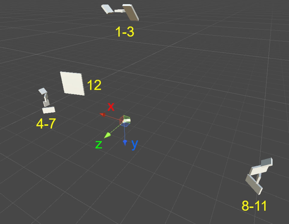
Overview for the simulated constellation of the reference geometries (grey planes) and the SOCS of the LS (RGB coordinate system) with respect to the actual experimental setup from section 4.1. The numbers indicate the e = 1 , … , 12 planes and a 1 m × 1 m grid is shown on the ground surface. The orientations and dimensions of the planes correspond to those in reality.

5.1 Simulated calibration data

The realisation and usage of simulated observations for the calibration of the LS with respect to the PCS allow statistical comparisons against the true nominal values. No large outliers were simulated within the model, but rather controlled conditions were established that correspond to the character of a well-controllable laboratory calibration. In order to make statistically verifiable statements, a closed-loop MC simulation (cf. [34]) is applied. Thus, a variety of slightly different realisations can be achieved. For this purpose, after simulating perfect 3D PCLs for both positions of the LS and assigning them to the individual e reference planes per epoch k, random subsampling is performed. As an additional variation, random normally distributed observation noise with a fixed value of 1 cm standard deviation for all axes is added within each of the S independent realisations. The following results refer to S = 1000 independently simulated data sets, each of which is evaluated using the different methodological calibration approaches.

At first, the required run time should be discussed, which is shown in Table 1 using the mean value over all S = 1000 realisations. The calculations were all performed in parallel on equivalent nodes as part of a computing cluster, allowing a relative comparison between the different methods to be made. The fastest mean run time for the recursive C-GHM (norm) is around 3.9 s. The main impact for the run time is the size of the normal equation system that has to be inverted. This depends directly on the number of 3D point observations used. Therefore, processing all observations at once in the batch C-GHM shows a significantly higher run time than all recursive methods. The temporal differences in the recursive methods in comparison arise because of the varying number of iterations until the abort criterion is satisfied within each epoch k. With regard to the standard deviations, it can also be seen that these slightly increase as a function of the mean run time. Here, the largest values are again clearly apparent for the batch approach.

In addition to the necessary run time, the actual calibration parameters are of interest. By knowing the true nominal values within the simulation, the root mean squared error (RMSE) serve as a statistical measure for comparing the different methods. The RMSE can be estimated within every S realisations for each epoch k according to

using the differences between the nominal values x ¯ and the estimated values x ˆ k , S . Here, the parameter n x indicates the number of state parameters used. The RMSE value can be specified with respect to individual elements of the state vector (e. g. translation in X direction), to aggregations (e. g. 3D translation) or to the whole set of state parameters. In each case, attention must be paid to the consideration of the corresponding units. Two different types of calculations are presented for the following results. One with respect to only the first six parameters (the 6-DoF calibration parameters between the SOCS of the LS and the PCS) and one with respect to the entire state vector with 66 elements, including all the plane parameters.

The results of the RMSE are presented in box plots grouped by the individual epochs. This is useful to show the whole set of results for all S realisations and reduces the impact of single failed runs or outliers at the same time. In a box plot, the circle indicates the median value, and the box describes all values between the 25th and 75th percentile. The whiskers span across all values in the range of 1.5 times the box interval. All other values are marked as outliers (red dots) but may only represent the tail end of the distribution. Due to the spread of resulting values, the vertical axis is scaled logarithmically. A comparison with the batch approach can be made by also calculating the RMSE for the estimated parameters and giving them independently of the epochs.

Figure 6 shows the results when the RMSE is based on the 6-DoF calibration parameters only. All recursive methods show comparable results since the median is almost identical. Therefore, there are no major improvements over the epochs in the recursive procedures. This indicates that additional observations have no significant influence on the parameters. It is noticeable, that the batch solution (last column) has a slightly smaller RMSE value, which is due to the entirety of observations taken into account at the same time.

Figure 6

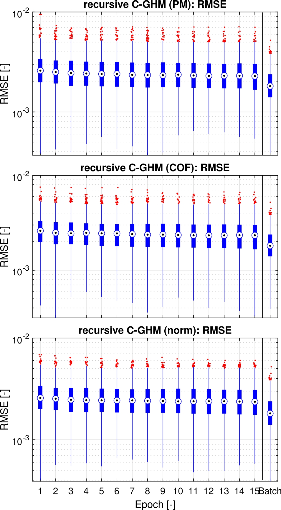
Box plot of the epoch wise RMSE for the LS pose of recursive C-GHM with perfect measurements (PM) and the constrained objective function (COF) and the recursive GHM with extended functional model (norm), all compared to the result of the batch processing in the last column. Vertical axis units are a combination of translations in meters and rotations in radians.

If the RMSE is determined on the basis of the entire state parameters, box plots as shown in Figure 7 are obtained. There is a slight increase in the RMSE values across all methods compared to Figure 6. In addition, all the investigated approaches behave identically and there is no change over the individual epochs. The previously occurring advantage of the batch approach is no longer present when the entire parameter vector is taken into account.

Figure 7

Box plot of the epoch wise RMSE for all parameters of recursive C-GHM with perfect measurements (PM) and the constrained objective function (COF) and the recursive GHM with extended functional model (norm), all compared to the result of the batch processing in the last column. Vertical axis units are a combination of translations in meters, rotations in radians and the plane parameters (normal vectors and distances in meters).

Furthermore, it is advisable to check consistency of the recursive filter approaches, which forms the basis for the recursive GHM. A state estimator is consistent if the estimates converge to the true value. Possible reasons why this is not the case are modeling, numerical or programming errors. A statistical test to verify the filter consistency is introduced in [1]. Since the true nominal values are known within the framework of this simulation, this verification is recommended. For this, the Normalized (state) estimation error squared (NEES) e k is defined as

where the differences between true state x ¯ k and estimated state x ˆ k are considered for each epoch k. In addition, a weighting is applied via the VCM Σ x ˆ x ˆ , k + of the states estimated. Since the random variable e k is a quadratic quantity, it is assumed that it follows a χ 2 distribution with u x degrees of freedom, indicating the number of states. Here, similar to the RMSE comparison, two different scenarios for u x are chosen. Once with respect to only the first six parameters and once with respect to the entire state vector with 66 elements. This χ 2 -test is accepted if

is fulfilled. In case of a significance level of α = 5 % and u x = 6 this will lead to the critical values r 1 and r 2

Figure 8 shows the NEES for the first six parameters. Generally, the behaviour is similar to that shown in Figure 6 when using the RMSE. The only difference is that the NEES value for the batch solution deviates slightly from the recursive values, but apart from the outliers it is always within the limits. The same applies to the recursive approaches. Also here, no changes can be detected over the individual epochs.

Figure 8

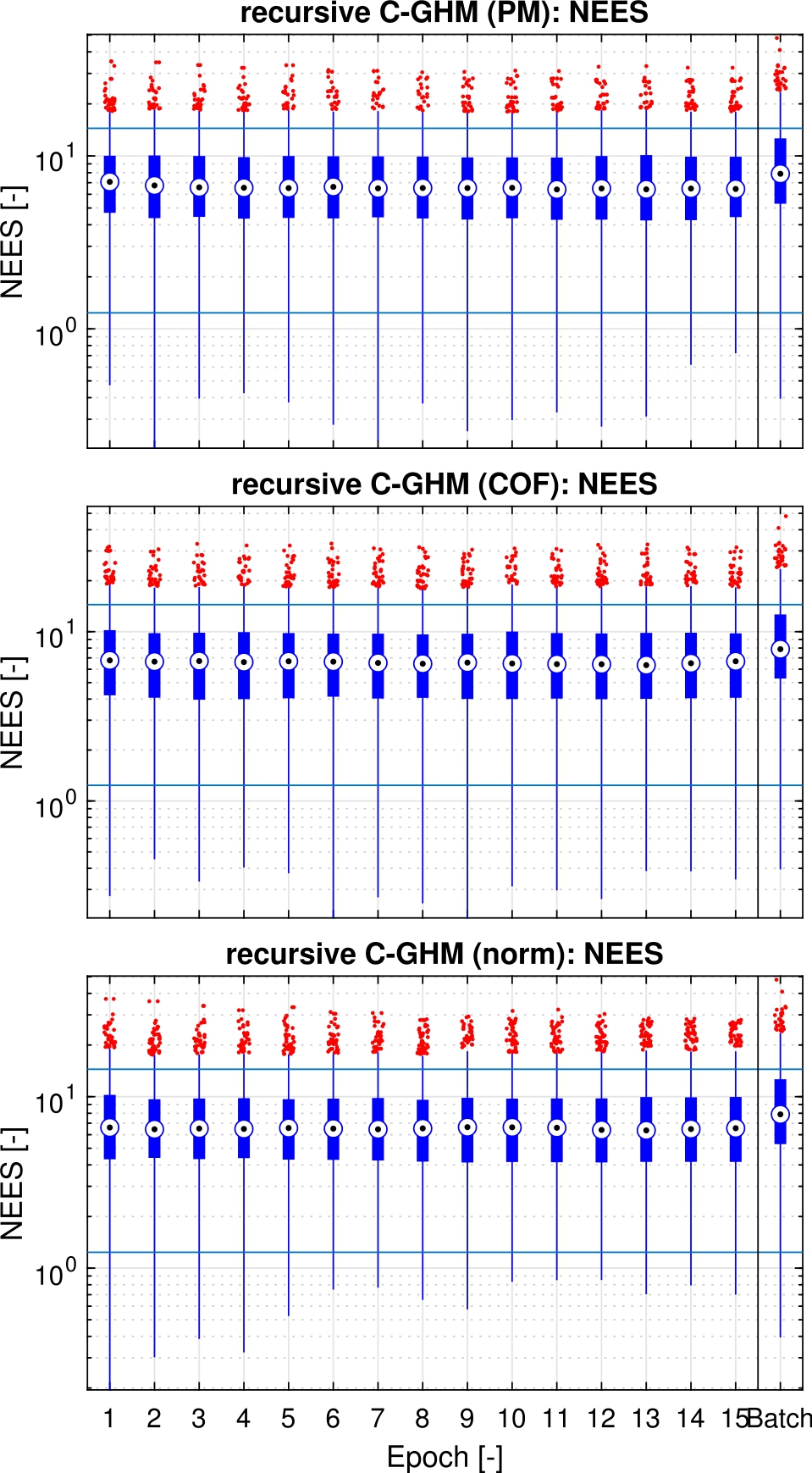
Box plot of the epoch wise NEES for the scanner pose of recursive C-GHM with perfect measurements and the constrained objective function and the recursive GHM with an extended functional model, all compared to the result of the batch processing in the last column, vertical axis units are a combination of translations in meters and rotations in radians. The borders of the acceptance intervals for the NEES are shown as horizontal lines.

Significantly different results are shown when the entire state vector for the NEES is considered. The results in this case are shown in Figure 9. Considering the complete state vector for the NEES leads to a significant increase in all the random variables, whereas for the RMSE, the change is only about one order of magnitude. Therefore, all test values are larger than the χ 2 consistency interval. A reason for this are too optimistic (co-)variances for the plane parameters. Over the individual epochs, all recursive methods show an improvement from the first to the second epoch, whereby this only improves further for the normalised method. A clear reason for this could not be found, even though this also indicates an over-optimistic VCM for the plane parameters in relation to the representation of the RMSE. Since the mentioned jump is not so strong in the approach with the normalised functional relationship, the consideration of constraints in the other two recursive methods may have an impact on this behaviour. Overall, the significantly more frequent occurrence of outliers in the recursive C-GHM with perfect measurements is striking. It becomes evident, that the numerical instabilities due to a partially ill-conditioned normal equation system only affect the additional parameters and not the actual 6-DoF calibration parameters, as can be seen in comparison with Figure 8.

Figure 9

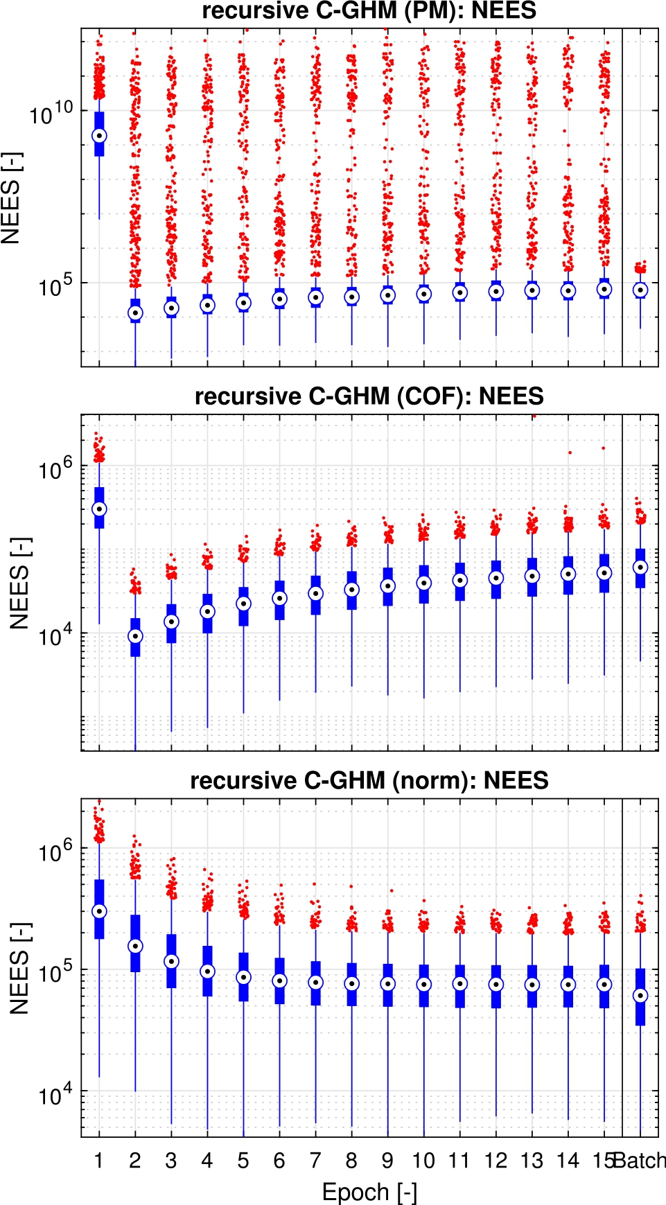
Box plot of the epoch wise NEES for all parameters of recursive C-GHM with perfect measurements and the constrained objective function and the recursive GHM with an extended functional model, all compared to the result of the batch processing in the last column. The vertical axis units combine translations in meters, rotations in radians and the plane parameters (normal vectors and distances in meters). The borders of the acceptance intervals for the NEES are shown as horizontal lines. Due to the logarithmic scale, these are no longer visible separately.

5.2 Real calibration data

In contrast to the simulated observation data in section 5.1, the nominal 6-DoF calibration parameters for the real observations are unknown. Furthermore, no reference values can be realised on the basis of a sensor of superior accuracy and precision since high-precision sensor technology, and state-of-the-art methods are already in use. As already mentioned above, the use of an MC simulation is therefore advisable. Thereby, many different data sets are realised, which differ exclusively based on the random subsampling of the LS observations. This enables an analysis of the scatter of the estimated parameters and a comparison between the individual methods.

The actual comparison at the level of the parameters is done exclusively for the translation t SOCS-PCS , x and the angle around this axis ω SOCS-PCS . For the other 6-DoF transformation parameters, the results are similar, although they are omitted here. For the recursive methods, the estimated value of the last epoch k = 15 is used. As discussed in section 5.1 the usage of the recursive C-GHM (PM) may lead to numerical issues with strongly deviating parameters in some of the 1000 independent realisations. For the used data set, the number of deviating realisations is less than 10. To compare the distributions of the resulting parameters, all values below the 0.5 % and above the 99.5 % quantiles were removed from the results of all methods. The remaining values are used to compute the statistics in Table 2. It can be noted that the batch solution reaches a minimum that differs by 1.7 mm for the translation and 0.03 ° for the rotation compared to the three recursive approaches. This deviation in the transformation parameters was already apparent previously on the basis of the RMSE in Figure 6. In addition, the slightly lower standard deviations for the batch method are noticeable, whereby this is clearly evident for the rotation.

The comparison of the different adjustment techniques in Table 2 is based on a variety of different subsampled realisations. However, this also provides insufficient insight into which approach best fits the true values. Thus, only conclusions regarding the precision of the individual approaches can be stated. Another possibility for a statistically verifiable analysis of the different methods without known nominal values is the application of a ( K-fold) cross-validation. According to [9], [10], [29], this method is based on the strategy of randomly assigning the available measurement data into K, exclusive of equally sized subsets (also referred to as folds) within a multitude of individual runs. Thus, all available observations are used, and no subsampling is carried out as before. Therefore, K − 1 subsets are selected and summarised as the training data set. The one remaining subset is referred to as the test data set. Using the larger training set, the unknown 6-DoF calibration parameters are estimated as before. Afterwards, the smaller test set is used to verify the results (by means of the contradictions d j e according to Equation (62)) based on the training set. This approach thus allows a relative comparison between the different approaches based on the distribution of the contradictions that occur. Subsequently, the assignment of the individual subsets to the two types of data sets changes K − 1 times and the contradictions are calculated again in each case. Overall, this procedure is referred to as one single run of the cross-validation. The usage of K-fold thus ensures that each observation is used once for testing. For statistically reliable statements, a multitude of such runs have to be performed, whereby the assignment of the original observation data to the K subsets is always random. All individual contradictions over all runs can then be represented in a histogram and the statistical central moments determined. For the investigations presented here, K = 10 is chosen, and a total of 100 runs are carried out. This allows a comprehensive distribution of the points and a variety of independent results within a feasible period of time.

The resulting large amount of observations prohibits timely processing with the batch C-GHM, so it is omitted and the investigations are only done between the recursive approaches. Instead, a recursive GHM without constraints is applied, whereas the referencing observations from the laser tracker are treated as deterministic variables. This can again indicate the added value of using geometric constraints. The histograms of all contradictions for the corresponding four recursive methods are shown in Figure 10. The contradictions of the recursive GHM without taking constraints into account show the most extensive spread in the results. In addition, a multimodal distribution and a slight bias can be identified for this approach. This is assumed to be caused by the LT observations, which were only considered as deterministic quantities in this specific approach. This behaviour thus illustrates the significance of estimating the additional parameters within the other methods, although this needs to be analysed in more detail in further investigations. Also, some of the contradictions are beyond the value range of ± 4 cm given here. This indicates that considering the laser tracker observations as stochastic variables leads to improved precision and accuracy of the adjustment. When constraints are taken into account, there are only minor differences in the results regarding the spread.

Figure 10

Histograms of the contradictions for the recursive approaches of the GHM, each with different consideration of constraints. The data is based on 100 independent 10-fold cross-validations for each approach.

5.3 Discussion

Based on the simulated and the real calibrations, the following findings can be made. In general, both the batch and the different recursive approaches do not differ significantly in terms of the 6-DoF calibration parameters. However, the required computation time is significantly lower with the recursive approach. This is a significant advantage, especially concerning larger data sets. In addition, it is shown that for the recursive calculation already one or two epochs can be sufficient for accurate calibration parameters. This can positively affect the required run time since additional observations do not necessarily lead to a steady improvement, at least in the application presented here. In this context, however, it is necessary to investigate in the future also for the batch approach to what extent the number of observations affects the quality of the parameters and the required computation times.

For the consideration of the constraints in the recursive approaches, it is noticeable that numerical instabilities in the PM method may cause wrong parameters conspicuously often. Consideration using the COF method and the normalized functional relationship are more reliable in this respect. The latter is characterized by the lowest overall run times but leads to less accurate estimates of the plane parameters. It has to be noted that the comparison of the plane parameters to the nominal values technically is not possible when using the normalized functional relationship. Because of the missing constraint, the parameters can just be scaled in comparison to the true values. However, the parameters of the reference geometries are consistently inaccurate with all applied methods. A reason for this behaviour could not be found. This situation is also shown because the calculated co-variances of the plane parameters are too optimistic and lead to an inconsistent estimation. However, if only the 6-DoF calibration parameters are considered, the consistency of the recursive estimator based on the χ 2 -test can be confirmed.

The general advantage of using constraints when calibrating with reference geometries is shown in the context of cross-validation. If the plane parameters are introduced as deterministic quantities, this leads to a significantly wider dispersion of the contradictions. The specific method by which the constraints are taken into account is of secondary importance. The accuracy and precision with respect to the pure 6-DoF calibration parameters are similar overall, although there are relevant differences with respect to the numerical stability.

The major advantage of the recursive C-GHM is the significant run time improvement compared with a batch approach. This can be of particular relevance for potential real-time applications or steadily increasing data sets. With respect to the calibration of an LS, for example, this may be the case if the sensor has multiple scan lines (e. g. Velodyne HDL-64 [59]), the calibration setup uses more individual reference geometries (for higher redundancy) or multiple individual positions (for decorrelation) for a more reliable estimation are used.

References

[1] Y. Bar-Shalom, X.-R. Li and T. Kirubarajan, Estimation with Applications to Tracking and Navigation: Theory, Algorithms and Software, Wiley, New York, NY, 2001.10.1002/0471221279Suche in Google Scholar
[2] W. Błaszczak-Bąk, Z. Koppanyi and C. Toth, Reduction Method for Mobile Laser Scanning Data, in: ISPRS Int. J. Geo-Inf., 7(7), pp. 1–13, 2018.10.3390/ijgi7070285Suche in Google Scholar
[3] J. M. Brockmann and W.-D. Schuh, Computational Aspects of High-resolution Global Gravity Field Determination–Numbering Schemes and Reordering, in: NIC Symposium 2016, No. FZJ-2016-02087, John von Neumann-Institut für Computing, 2016.Suche in Google Scholar
[4] Y.-T. Chiang, L.-S. Wang and F.-R. Chang, Filtering Method for Nonlinear Systems with Constraints, in: IEEE Proceedings – Control Theory and Applications, 149(6), pp. 525–531, 2002.10.1049/ip-cta:20020799Suche in Google Scholar
[5] T. Dang, Kontinuierliche Selbstkalibrierung von Stereokameras, Ph. D. Thesis, Schriftenreihe / Institut für Mess- und Regelungstechnik, KIT, Univ.-Verl. Karlsruhe, Karlsruhe, 2007.Suche in Google Scholar
[6] T. Dang, An Iterative Parameter Estimation Method for Observation Models with Nonlinear Constraints, in: Metrology and Measurement Systems, 15(4), pp. 421–432, 2008.Suche in Google Scholar
[7] W. F. Denham and S. Pines, Sequential Estimation When Measurement Function Nonlinearity Is Comparable to Measurement Error, in: AIAA Journal, 4(6), pp. 1071–1076, 1966.10.2514/6.1965-1220Suche in Google Scholar
[8] X. Du and Y. Zhuo, A Point Cloud Data Reduction Method Based on Curvature, in: 2009 IEEE 10th International Conference on Computer-Aided Industrial Design & Conceptual Design, pp. 914–918, 2009.10.1109/CAIDCD.2009.5375038Suche in Google Scholar
[9] B. Efron and R. Tibshirani, An Introduction to the Bootstrap, Chapman & Hall, New York, 1993.10.1007/978-1-4899-4541-9Suche in Google Scholar
[10] B. Efron and T. Hastie, Computer Age Statistical Inference: Algorithms, Evidence, and Data Science, Institute of Mathematical Statistics monographs, Cambridge University Press, New York, 2016.10.1017/CBO9781316576533Suche in Google Scholar
[11] J. Elseberg, D. Borrmann and A. Nüchter, Algorithmic Solutions for Computing Precise Maximum Likelihood 3d Point Clouds from Mobile Laser Scanning Platforms, in: Remote Sensing, 5(11), pp. 5871–5906, 2013.10.3390/rs5115871Suche in Google Scholar
[12] J. Elseberg, D. Borrmann and A. Nüchter, One Billion Points in the Cloud – an Octree for Efficient Processing of 3D Laser Scans, in: ISPRS Journal of Photogrammetry and Remote Sensing, 76, pp. 76–88, 2013.10.1016/j.isprsjprs.2012.10.004Suche in Google Scholar
[13] D. Ernst, Objektraumbasierte Kalibrierung und Georeferenzierung eines Unmanned Aerial Systems, Bachelor Thesis (unpublished), Leibniz Universität Hannover, Hanover, 2019.Suche in Google Scholar
[14] A. Ettlinger, H. Neuner and T. Burgess, Development of a Kalman Filter in the Gauss-helmert Model for Reliability Analysis in Orientation Determination with Smartphone Sensors, in: Sensors, 18(2), 414, pp. 1–21, 2018.10.3390/s18020414Suche in Google Scholar PubMed PubMed Central
[15] N. Garcia-Fernandez, H. Alkhatib and S. Schön, Collaborative Navigation Simulation Tool Using Kalman Filter with Implicit Constraints, in: ISPRS Annals of Photogrammetry, Remote Sensing and Spatial Information Sciences, IV-2/W5, pp. 559–566, 2019.10.5194/isprs-annals-IV-2-W5-559-2019Suche in Google Scholar
[16] J. de Geeter, H. van Brussel, J. de Schutter and M. Decreton, A Smoothly Constrained Kalman Filter, in: IEEE Transactions on Pattern Analysis and Machine Intelligence, 19(10), pp. 1171–1177, 1997.10.1109/34.625129Suche in Google Scholar
[17] G. Gräfe, Kinematische Anwendungen von Laserscannern im Straßenraum, Ph. D. Thesis, Issue 84, Universität der Bundeswehr München, Fakultät für Bauingenieur- und Vermessungswesen, Neubiberg, 2007.Suche in Google Scholar
[18] N. Gupta and R. Hauser, Kalman Filtering with Equality and Inequality State Constraints, https://arxiv.org/abs/0709.2791, Accessed: 2019-10-05, 2007.Suche in Google Scholar
[19] J. Hartmann, J.-A. Paffenholz, T. Strübing and I. Neumann, Determination of Position and Orientation of Lidar Sensors on Multisensor Platforms, in: Journal of Surveying Engineering, 143(4), pp. 1–11, 2017.10.1061/(ASCE)SU.1943-5428.0000226Suche in Google Scholar
[20] J. Hartmann, P. Trusheim, H. Alkhatib, J.-A. Paffenholz, D. Diener and I. Neumann, High Accurate Pointwise (Geo-)Referencing of a k-TLS Based Multi-sensor-system, in: ISPRS Annals of Photogrammetry, Remote Sensing and Spatial Information Sciences, IV-4, pp. 81–88, 2018.10.5194/isprs-annals-IV-4-81-2018Suche in Google Scholar
[21] J. Hartmann, I. von Gösseln, N. Schild, A. Dorndorf, J.-A. Paffenholz and I. Neumann, Optimisation of the Calibration Process of a k-TLS Based Multi-sensor-system by Genetic Algorithms, in: ISPRS – International Archives of the Photogrammetry, Remote Sensing and Spatial Information Sciences, XLII-2/W13, pp. 1655–1662, 2019.10.5194/isprs-archives-XLII-2-W13-1655-2019Suche in Google Scholar
[22] A. Heiker, Mutual Validation of Earth Orientation Parameters, Geophysical Excitation Functions and Second Degree Gravity Field Coefficients, Ph. D. Thesis, DGK, Reihe C, 697, Munich, 2013.Suche in Google Scholar
[23] E. Heinz, C. Holst, H. Kuhlmann and L. Klingbeil, Design and Evaluation of a Permanently Installed Plane-based Calibration Field for Mobile Laser Scanning Systems, in: Remote Sensing, 12(3), pp. 1–29, 2020.10.3390/rs12030555Suche in Google Scholar
[24] C. Hesse, Hochauflösende kinematische Objekterfassung mit terrestrischen Laserscannern, Ph. D. Thesis, DGK, Reihe C, 608, Munich, 2007.Suche in Google Scholar
[25] Hexagone Metrology, Leica Absolute Tracker AT960 (Product Brochure): Absolute Portability. Absolute Speed. Absolute Accuracy, https://w3.leica-geosystems.com/downloads123/m1/metrology/general/brochures/leica%20at960%20brochure_en.pdf, Accessed: 2020-02-05.Suche in Google Scholar
[26] G. H. Hostetter, Recursive Estimation, in: Handbook of Digital Signal Processing, Academic Press, pp. 899–940, 1987.10.1016/B978-0-08-050780-4.50018-7Suche in Google Scholar
[27] Ibeo Automotive Systems, ibeoNEXT Generic 4D Solid State LiDAR: Die Zukunft des autonomen Fahrens!, https://www.ibeo-as.com/de/produkte/sensoren/ibeoNEXTgeneric, 2020, Accessed: 2020-02-06.Suche in Google Scholar
[28] R. Jäger, T. Müller, H. Saler and R. Schwäble, Klassische und robuste Ausgleichungsverfahren: Ein Leitfaden für Ausbildung und Praxis von Geodäten und Geoinformatikern, Wichmann, Heidelberg, 2005.Suche in Google Scholar
[29] G. James, D. Witten, T. Hastie and R. Tibshirani, An Introduction to Statistical Learning: With Applications in R, Springer, New York, Heidelberg, Dordrecht, London, 2017.Suche in Google Scholar
[30] R. E. Kalman and R. S. Bucy, New Results in Linear Filtering and Prediction Theory, in: Journal of Basic Engineering, 83(1), pp. 95–108, 1961.10.1115/1.3658902Suche in Google Scholar
[31] R. Klees, P. Ditmar and J. Kusche, Numerical Techniques for Large Least-squares Problems with Applications to Goce, in: V Hotine-Marussi Symposium on Mathematical Geodesy, Springer, Berlin, Heidelberg, pp. 12–21, 2004.10.1007/978-3-662-10735-5_3Suche in Google Scholar
[32] K.-R. Koch, Parameter Estimation and Hypothesis Testing in Linear Models, Springer, Berlin, Heidelberg, 1999.10.1007/978-3-662-03976-2Suche in Google Scholar
[33] K.-R. Koch, Robust estimations for the nonlinear Gauss Helmert model by the expectation maximization algorithm, in: Journal of Geodesy, 88(3), pp. 263–271, 2014.10.1007/s00190-013-0681-9Suche in Google Scholar
[34] D. P. Kroese, T. Taimre and Z. I. Botev, Handbook of Monte Carlo Methods, John Wiley & Sons, 2011.10.1002/9781118014967Suche in Google Scholar
[35] L. Lenzmann and E. Lenzmann, Strenge Auswertung des nichtlinearen Gauß-Helmert-Modells, in: AVN (Allgemeine Vermessungs-Nachrichten), 111(2), pp. 68–73, 2004.Suche in Google Scholar
[36] M. Lösler and M. Nitschke, Bestimmung der Parameter einer Regressionsellipse in allgemeiner Raumlage, in: AVN (Allgemeine Vermessungs-Nachrichten), 117(3), pp. 113–117, 2010.Suche in Google Scholar
[37] R. P. Lutter and T. Olson, Multi-Sensor System, US 6771208 B2, https://patents.google.com/patent/US6771208, 2004, Accessed: 2020-02-06.Suche in Google Scholar
[38] J. E. Mulquiney, J. P. Norton, A. J. Jakeman and J. A. Taylor, Random Walks in the Kalman Filter: Implications for Greenhouse Gas Flux Deductions, in: Environmetrics, 6(5), pp. 473–478, 1995.10.1002/env.3170060509Suche in Google Scholar
[39] W. Niemeier, Ausgleichungsrechnung: Statistische Auswertemethoden, De Gruyter, Berlin, 2008.10.1515/9783110206784Suche in Google Scholar
[40] T. Peters and C. Brenner, Conditional Adversarial Networks for Multimodal Photo-realistic Point Cloud Rendering, in: M. Raubal, S. Wang, M. Guo, D. Jonietz, and P. Kiefer, Editors, Spatial Big Data and Machine Learning in GIScience, GIScience Workshop 2018, Melbourne, Australia, pp. 48–53, 2018.Suche in Google Scholar
[41] R. L. Plackett, Some Theorems in Least Squares, in: Biometrika, 37(1/2), pp. 149–157, 1950.10.1093/biomet/37.1-2.149Suche in Google Scholar
[42] J. Porrill, Optimal Combination and Constraints for Geometrical Sensor Data, in: The International Journal of Robotics Research, 7(6), pp. 66–77, 1988.10.1177/027836498800700606Suche in Google Scholar
[43] E. Puttonen, M. Lehtomäki, H. Kaartinen, L. Zhu, A. Kukko and A. Jaakkola, Improved Sampling for Terrestrial and Mobile Laser Scanner Point Cloud Data, in: Remote Sensing, 5(4), pp. 1754–1773, 2013.10.3390/rs5041754Suche in Google Scholar
[44] A. Rietdorf, Automatisierte Auswertung und Kalibrierung von scannenden Messsystemen mit tachymetrischem Messprinzip, Ph. D. Thesis, DGK, Reihe C, 582, Munich, 2005.Suche in Google Scholar
[45] Robosense, RS-LiDAR-32, https://www.robosense.ai/rslidar/rs-lidar-32, 2020, Accessed: 2020-02-06.Suche in Google Scholar
[46] L. R. Roese-Koerner, Convex Optimization for Inequality Constrained Adjustment Problems, Ph. D. Thesis, DGK, Reihe C, 759, Munich, 2015.Suche in Google Scholar
[47] L. R. Roese-Koerner, B. Devaraju, W.-D. Schuh and N. Sneeuw, Describing the Quality of Inequality Constrained Estimates, in: The 1st International Workshop on the Quality of Geodetic Observation and Monitoring Systems (QuGOMS’11), pp. 15–20, 2015.10.1007/978-3-319-10828-5_3Suche in Google Scholar
[48] S. Schön, C. Brenner, H. Alkhatib, M. Coenen, H. Dbouk, N. Garcia-Fernandez, C. Fischer, C. Heipke, K. Lohmann, I. Neumann, U. Nguyen, J.-A. Paffenholz, T. Peters, F. Rottensteiner, J. Schachtschneider, M. Sester, L. Sun, S. Vogel, R. Voges and B. Wagner, Integrity and Collaboration in Dynamic Sensor Networks, in: Sensors, 18(7), pp. 1–21, 2018.10.3390/s18072400Suche in Google Scholar PubMed PubMed Central
[49] K. P. Schwarz and N. El-Sheimy, Kinematic Multi-sensor Systems For Close Range Digital Imaging, in: ISPRS International Archives of the Photogrammetry, Remote Sensing and Spatial Information Sciences, XXXI-5/W3, pp. 774–784, 1996.Suche in Google Scholar
[50] D. Simon, Optimal State Estimation, John Wiley & Sons, New Jersey, 2006.10.1002/0470045345Suche in Google Scholar
[51] D. Simon, Kalman Filtering with State Constraints: A Survey of Linear and Nonlinear Algorithms, in: IET Control Theory & Applications, 4(8), pp. 1303–1318, 2010.10.1049/iet-cta.2009.0032Suche in Google Scholar
[52] S. Soatto, R. Frezza and P. Perona, Motion Estimation on the Essential Manifold, in: Computer vision – ECCV’94, Lecture Notes in Computer Science, Volume 801, pp. 60–72, Springer, Berlin, 1994.10.1007/BFb0028335Suche in Google Scholar
[53] R. Steffen and C. Beder, Recursive Estimation with Implicit Constraints, in: F. A. Hamprecht, C. Schnörr and B. Jähne, Editors, Pattern Recognition, Lecture Notes in Computer Science, Volume 4713, pp. 194–203, Springer, Berlin, 2007.10.1007/978-3-540-74936-3_20Suche in Google Scholar
[54] R. Steffen, A Robust Iterative Kalman Filter Based On Implicit Measurement Equations, in: Photogrammetrie – Fernerkundung – Geoinformation, pp. 323–332, 2013.10.1127/1432-8364/2013/0180Suche in Google Scholar
[55] R. Steffen, Visual Slam from Image Sequences Acquired by Unmanned Aerial Vehicles, Ph. D. Thesis, DGK, Reihe C, 709, Munich, 2013.Suche in Google Scholar
[56] T. Strübing and I. Neumann, Positions- und Orientierungsschätzung von LIDAR-Sensoren auf Multisensorplattformen, in: Zeitschrift für Geodäsie, Geoinformation und Landmanagement, 138(3), pp. 210–221, 2013.Suche in Google Scholar
[57] C. Suchocki and W. Blaszczak-Bak, Down-sampling of Point Clouds for the Technical Diagnostics of Buildings and Structures, in: Geosciences, 9(2), 2019.10.3390/geosciences9020070Suche in Google Scholar
[58] J. Underwood, A. Hill and S. Scheding, Calibration of Range Sensor Pose on Mobile Platforms, in: IEEE/RSJ International Conference on Intelligent Robots and Systems, Piscataway, NJ, pp. 3866–3871, 2007.10.1109/IROS.2007.4398971Suche in Google Scholar
[59] Velodyne LiDAR, Datasheet: HDL-64E: High Definition Real-time 3D Lidar, https://velodynelidar.com/products/hdl-64e/, 2018, Accessed: 2020-02-06.Suche in Google Scholar
[60] Velodyne LiDAR, Datasheet: Velodyne LiDAR Puck: Real-Time 3D LiDAR Sensor, https://velodynelidar.com/vlp-16.html, 2018, Assessed: 2019-12-12.Suche in Google Scholar
[61] H. Vennegeerts, Objektraumgestützte kinematische Georeferenzierung für Mobile-Mapping-Systeme, Ph. D. Thesis, DGK, Reihe C, 657, Munich, 2011.Suche in Google Scholar
[62] S. Vogel, H. Alkhatib and I. Neumann, Iterated Extended Kalman Filter with Implicit Measurement Equation and Nonlinear Constraints for Information-based Georeferencing, in: 21st IEEE International Conference on Information Fusion (FUSION), Cambridge, United Kingdom, pp. 1209–1216, 2018.10.23919/ICIF.2018.8455258Suche in Google Scholar
[63] S. Vogel, H. Alkhatib, J. Bureick, R. Moftizadeh and I. Neumann, Georeferencing of Laser Scanner-based Kinematic Multi-sensor Systems in the Context of Iterated Extended Kalman Filters Using Geometrical Constraints, in: Sensors, 19(10), pp. 1–22, 2019.10.3390/s19102280Suche in Google Scholar PubMed PubMed Central
[64] S. Vogel, Kalman Filtering with State Constraints Applied to Multi-sensor Systems and Georeferencing, Ph. D. Thesis, DGK, Reihe C, 856, Munich, 2020.Suche in Google Scholar
[65] Y. Wang, Q. Chen, Q. Zhu, L. Liu, C. Li and D. Zheng, A Survey of Mobile Laser Scanning Applications and Key Techniques over Urban Areas, in: Remote Sensing, 11(13), pp. 1–20, 2019.10.3390/rs11131540Suche in Google Scholar
[66] K. Wichmann, Auswertung von Messdaten: Statistische Methoden für Geo- und Ingenieurwissenschaften, De Gruyter, Munich, 2007.10.1524/9783486844184Suche in Google Scholar
© 2022 Vogel et al., published by De Gruyter
This work is licensed under the Creative Commons Attribution 4.0 International License.
Artikel in diesem Heft
- Frontmatter
- Research Articles
- Multiple incompatible datum points identification in vertical control network for high-speed railway based on likelihood ratio test
- Empirical influence functions and their non-standard applications
- Multi-frequency quadrifilar helix antennas for cm-accurate GNSS positioning