Prognostic adjustment with efficient estimators to unbiasedly leverage historical data in randomized trials
-
Lauren D. Liao
 ,
Emilie Højbjerre-Frandsen
,
Emilie Højbjerre-Frandsen

Abstract
Although randomized controlled trials (RCTs) are a cornerstone of comparative effectiveness, they typically have much smaller sample size than observational studies due to financial and ethical considerations. Therefore there is interest in using plentiful historical data (either observational data or prior trials) to reduce trial sizes. Previous estimators developed for this purpose rely on unrealistic assumptions, without which the added data can bias the treatment effect estimate. Recent work proposed an alternative method (prognostic covariate adjustment) that imposes no additional assumptions and increases efficiency in trial analyses. The idea is to use historical data to learn a prognostic model: a regression of the outcome onto the covariates. The predictions from this model, generated from the RCT subjects’ baseline variables, are then used as a covariate in a linear regression analysis of the trial data. In this work, we extend prognostic adjustment to trial analyses with nonparametric efficient estimators, which are more powerful than linear regression. We provide theory that explains why prognostic adjustment improves small-sample point estimation and inference without any possibility of bias. Simulations corroborate the theory: efficient estimators using prognostic adjustment compared to without provides greater power (i.e., smaller standard errors) when the trial is small. Population shifts between historical and trial data attenuate benefits but do not introduce bias. We showcase our estimator using clinical trial data provided by Novo Nordisk A/S that evaluates insulin therapy for individuals with type 2 diabetes.
1 Introduction
Practical, financial, and ethical concerns often preclude large randomized trials, which limits their power [1], [2], [3]. On the other hand, historical (often observational) data are often plentiful, and there are many existing methods for including historical data in trial analyses in order to boost power [4]. “Data fusion” methods simply pool trials with historical data [5], [6], [7]. Bayesian methods, which naturally rely on assumptions in the form of specified priors from historical data, are also popular in the literature [8], 9]. Similar problems have also been addressed in the generalizability and transportability research [6], 10], 11]. Recent studies proposed machine learning methods to integrate prior observational studies into trial analyses [12], 13]. Although pooled-estimators are an active research field – integrating historical with trial data, (for example, Dang et al. [14]) we focus on improving trial analysis alone.
Unfortunately, the aforementioned approaches that rely on validity of historical data are all sensitive to unobservable selection biases and must therefore be used with extreme care. The fundamental problem is that the historical population may differ systematically from the trial population in ways that impact both treatment assignment and outcome. For example, if the historical population did not have access to a modern standard-of-care, adding historical controls would artificially make any new drug seem more effective than it really is. Observable differences in populations can potentially be corrected under reasonable assumptions, but shifts in unobserved variables are impossible to detect or correct.
We take the approach of covariate adjustment to increase efficiency. In recognition of using covariates to reduce estimation uncertainty, the U.S. Food and Drug Adminstration recently released guidance on adjusting for covariates in randomized clinical trials [15]. See Van et al. [16] for summarized methods using covariate adjustment [16]. Our research builds on Schuler et al. [17], who suggest using the historical data to train a prognostic model that predicts the outcome from baseline covariates [17]. They then adjust for the model’s predictions on the trial data in the trial analysis using linear regression, namely the “prognostic adjustment”. A similar research proposed by Holzhauer and Adewuyi [18] recommends using a “super-covariate,” combining multiple prognostic models into a single covariate for adjustment [18]. However, both these methods are limited to trial analyses using linear regression models.
Our task in this paper is to extend the prognostic adjustment approach beyond linear regression, specifically, to “semiparametrically efficient” estimators. Semiparametrically efficient estimators are those that attain the semiparametric efficient variance bound, which is the smallest asymptotic variance that any estimator can attain. The use of efficient estimators thus tends to reduce the uncertainty of the treatment effect estimate. These estimators leverage machine learning internally to estimate the treatment or the outcome model, or both; for example, the augmented inverse probability weighting estimator (AIPW) and the targeted maximum likelihood estimator (TMLE) are commonly used to evaluate the average treatment effect [19], [20], [21], [22], [23]. These estimators have been shown to improve the power of trials over unadjusted or linearly adjusted estimates [24].
In this study, we aim to improve power even further by incorporating historical data via prognostic adjustment. Our approach guarantees asymptotic efficiency of the trial treatment effect and more importantly, promises benefits in small-sample efficiency and robust inference.
2 Framework and notation
We follow the causal inference framework and roadmap from Petersen and van der Laan [25]. First, we define each observational unit i ∈ {1, …, n}, as an independent, identically distributed random variable, O
i
with true distribution P. In our setting, each random variable O = (W, A, Y, D) contains associated p baseline covariates
We will assume that the trial data is generated under the setting of an RCT, such that P (A = a|W, D = 1) = π a , with some positive constant π a denoting the treatment probability for a ∈ {0, 1}. Define μ a (W) = E P [Y|A = a, W, D = 1] as the conditional outcome means per treatment arm in the trial. Let ρ d (W) = E [Y|W, D = d] denote the prognostic score for a dataset d [26]. When referenced without subscript (ρ) we are referring to the prognostic score in the historical data D = 0.
The fundamental problem of causal inference comes from not being able to observe the outcome under both treatment types. We assume that for each individual, Y = Y(A), i.e., we observe the potential outcome corresponding to the observed treatment. To calculate the causal parameter of interest, we define the (unobservable) causal data to be (Y 1, Y 0, A, W, D), generated from a causal data generating distribution P*. In this study, we are interested in the causal average treatment effect (ATE) in the trial population:
which due to randomization in the trial is equal to the observable quantity:
where μ a (W) = E P [Y|A = a, W, D = 1] is the conditional mean outcome in treatment arm a ∈ {0, 1} from the observable data distribution.
Let (W, Y) denote a dataset with observed outcome Y = [Y
1, …, Y
n
] and the observed covariates W = [W
1, …, W
n
], where
3 Proposed method
3.1 Efficient estimators with prognostic score adjustment
Our proposed method for incorporating historical data with efficient estimators is simple: we first obtain a prognostic model by performing an outcome prediction to fit the historical data (D = 0) using a machine learning algorithm
In practice, we suggest using a cross-validated ensemble algorithm (also called “super-learner”) for
For an efficient estimator, adding a fixed function of the covariates as an additional covariate will not change the asymptotic behavior [30], 31]. Thus our approach will never be worse than ignoring the historical data (as it might be if we pooled the data to learn the outcome regression). However, it also means that our approach cannot reduce asymptotic variance (indeed it is impossible to do so without making assumptions).
Nonetheless, we find that the finite-sample variance of efficient estimators is far enough from the efficiency bound that using the prognostic score as a covariate generally decreases the variance (without introducing bias) and improves estimation of the standard error. Mechanistically, this happens because the prognostic score “jump-starts” the learning curve of the outcome regression models such that more accurate predictions can be made with fewer trial data. This is especially true when the outcome-covariate relationship is complex and difficult to learn from a small trial. It is well-known that the performance of efficient estimators in RCTs is dependant on the predictive power of the outcome regression. Therefore improving this regression (by leveraging historical data) can reduce variance.
We expect finite-sample benefits as long the trial and historical populations and treatments are similar enough. But even if they are not identical, the prognostic score is still likely to contain very useful information about the conditional outcome mean.
In the following Subsections 3.2 to 3.5, we theoretically show how adjusting for a prognostic score with an efficient estimator can improve estimation in a randomized trial. In an asymptotic analysis where the historical data grows much faster than the trial data, we show that using the prognostic score speeds the decay of the empirical process term in the stochastic decomposition of our estimator. The implications are that small-sample point estimation and inference should be improved even though efficiency gains will diminish asymptotically. The material assumes expertise with semiparametric efficiency theory and targeted/double machine learning. We present our results at a high level and do not present enough background details for readers not specialized in semiparametric inference. Two good starting points for this material are Schuler and van der Laan and Kennedy [32], 33]. The casual reader may skip this section and if they are comfortable with the above heuristic explanation of why prognostic adjustment may improve performance.
3.2 No asymptotic efficiency gain
Before showing how adjusting for a prognostic score for an efficient estimator can benefit estimation, we show that adding any prognostic score to an efficient estimator cannot improve asymptotic efficiency. To see this, we will start by considering the counterfactual means ψ a = E [E [Y|A = a, W]] = E [μ a (W)] for any choice of a ∈ {0, 1}. We will return to the ATE shortly, but for now, it will make our argument clearer to only consider counterfactual means. Consider any efficient estimator for ψ a in a semiparametric model (known treatment mechanism) over the trial data (Y, A, W). The influence function of an estimator completely determines its asymptotic behavior. By definition, any efficient estimator of E [μ a (W)] must have an influence function equal to the canonical gradient, which is referred to as the efficient influence function:
where I is the indicator function and π a = P (A = a) is the fixed, known propensity score.
The efficient influence function in an RCT (where the propensity score is known) is the same as for an observational study (where the propensity score is unknown) as shown by Hahn [34]. Consider now a distribution over (Y, A [W, R]), where R = g(W) for any fixed function g playing the role of a prognostic model. The efficient influence function in this setting is the same as the above. To see this formally one must observe that the tangent space of the factor P (R|Y, A, W) is {0} and does not contribute to the projection of the influence function of e.g. the difference-in-means estimator. Intuitively this is because observing R = g(W) does not add any additional information that can be exploited since it is a fixed, known transformation of the observed covariates.
The fundamental issue is that the asymptotic efficiency bound cannot be improved without considering a different statistical model, e.g. distributions over (Y, A, W, D). The problem is that in considering a different model we must also introduce additional assumptions to maintain identifiability of our trial-population causal parameter. For example, Li et al. [13] consider precisely this setup and rely on an assumption of “conditional mean equivalence” E [Y|A, W, D = 1] = E [Y|A, W, D = 0] to maintain identification while improving efficiency [13]. Similarly, an analysis following Chakrabortty et al. [35] shows that efficiency gains are also possible if we assume the covariate distributions are the same when conditioning on D [35]. In this paper, we take the covariate adjustment approach, incorporating the external data without these explicit assumptions and therefore we have to look for benefits in finite sample improvements.
3.3 Improving point estimation
To understand the benefits of prognostic adjustment we must consider the non-asymptotic behavior of our estimator. As above we will consider estimation of the treatment-specific mean ψ a , but from now on we will omit the a subscripts to reduce visual clutter.
Consider the following decomposition:
This sort of decomposition is common in the analysis of efficient estimators [32], 33]. As above, ϕ here denotes the efficient influence function of ψ. We use the empirical process notation
Of the remaining terms, the first is the efficient influence function term, P
n
ϕ. We have already shown that an efficient estimator leveraging the prognostic score has the same influence function as one without. It is also known that the remainder term
That leaves us with only the “empirical process” term
We can formalize this asymptotically. Recall that n denotes the trial sample size and
Instead of fitting our trial outcome regression with the prognostic score as a covariate, presume that we directly take
The result of making the empirical process term higher order is to reduce finite-sample variance of our point estimate. With cross-fitting the empirical process term is exactly mean-zero [32], 33], so finite-sample bias is unaffected.
3.4 Improving standard error estimation
We can apply similar arguments to show that the performance of the plug-in estimate of asymptotic variance
The first term here is a nice empirical mean which by the central limit goes to zero at a root-n rate and is unaffected by prognostic adjustment. The second term is similar to the empirical process term discussed above in the context of point estimation and by identical arguments this term decays faster when prognostic adjustment is used (note L
2 convergence of
The last term is bounded by
3.5 Caveats
Although we do not need additional assumptions for identifiability and thus retain unbiased estimation in all cases, all of the possible benefits described above do rely on the assumption that the historical and trial data-generating processes share a control-specific conditional mean. If this is not the case, then the amount by which the prognostic score speeds convergence of the control outcome regression will be attenuated, but not necessarily eliminated. For example, if the true outcome regression is the same as the prognostic score up to some parametric transformation that is learnable at a fast rate by a learner in our library
Until now we have also focused on the control counterfactual mean. The influence function for the ATE is the difference of those for the two counterfactual means and consequently we can decompose the empirical process term into two terms which are
Our analysis shows that use of the historical sample via prognostic score adjustment produces less-variable point estimates in small samples as well as more stable and accurate estimates of standard error. Unfortunately, asymptotic gains in efficiency are not possible without further assumptions.
However, these benefits are contingent on the extent to which the covariate-outcome relationships in both treatment arms of the trial are similar to the equivalent relationship in the historical data. In particular, differences between historical and trial populations and high heterogeneity of effect may both attenuate benefits. Nonetheless, these problems can never induce bias. Therefore, relative to alternatives, prognostic adjustment of efficient estimators provides strict guarantees for type I error, but at the cost of limiting the possible benefits of using historical data.
4 Simulation study
4.1 Setup
This simulation study aims to demonstrate the utility of an efficient estimator with the addition of a prognostic score. We examine how our method performs in different data generating scenarios (e.g., heterogeneous vs. constant effect), across different data set sizes, and when there are distributional shifts from the historical to the trial population. The simulation study is based on the structural causal model in DGP [1], [2], [3], [4], [5], [6], [7], [8], [9], [10]. In total there are 20 observed covariates of various types and a single unobserved covariate.
Notice that m a (W, U) is the mean of the counterfactual conditioned on both the observed and unobserved covariates. Our observable conditional means are thus μ a (W) = E [m a (W, U)|W]. We examine two different scenarios for the conditional outcome mean m a . In our “heterogeneous effect” simulation:
where the I represents the indicator function and propensity score π is written without the subscript a since the treatment probability is the same. To illustrate our results with another specification, we also include a second “heterogeneous effect” simulation to illustrate our results.
Our “constant effect” simulation is computed as:
To begin, we use the same data generating process (DGP) for the historical and trial populations except the fact that A = 0 deterministically in the historical DGP. But in what follows, we loosen this assumption by changing the historical data generating distribution with varying degrees of observed and unobserved covariate shifts.
We examine several scenarios: first, we analyze the trial (n = 250) under the heterogeneous and constant treatment effect DGPs, where the historical sample (
Third, we examine the effect of distributional shifts between the historical and trial populations. In these cases, we draw trial data from the DGP [1], [2], [3], [4], [5], [6], [7], [8], [9], [10], but draw our historical data from modified versions. To simulate a “small” observable population shift we let W 1|D = 0 ∼Unif (−5, − 2) and to simulate a “large” observable population shift we let W 1|D = 0 ∼Unif (−7, − 4). To simulate a “small” unobservable population shift we let U|D = 0 ∼Unif (0.5, 1.5) and to simulate a “large” unobservable population shift we let U|D = 0 ∼Unif [1], 2]. The shifts in the unobserved covariate induce shifts in the conditional mean relationship between the observed covariates and the outcome (see Supplemental Appendix A for an explicit explanation).
We consider three estimators for the trial: unadjusted (difference-in-group-means), main terms only linear regression (with Huber-White (robust) standard errors estimator HC3 [36], [37], [38], and targeted maximum likelihood estimation (TMLE; an efficient estimator [19]). All estimators return an effect estimate and an estimated standard error, which we use to construct Wald 95 % confidence intervals and corresponding p-values. The naive unadjusted estimator cannot leverage any covariates, but both linear and TMLE estimators can. We compare and contrast results from linear and TMLE estimators both with and without the fitted prognostic score as an adjustment covariate (“fitted”) to compare against Schuler et al. [17]. We also consider the oracle version of the prognostic score (“oracle”) for a benchmark comparison; the oracle prognostic score perfectly models the expected control outcome in the trial E [Y|W, A = 0, D = 0]. Unlike the fit prognostic score, the oracle version is not affected by random noise in the historical data and it is not sensitive to shifts between historical and trial populations (indeed it is not affected by the historical data at all). The oracle prognostic score only serves as a best-case comparison and is infeasible to calculate in practice.
For simplification, we include the same specifications of the discrete super learner (cross-validated ensemble algorithm) for both the prognostic model and all regressions required by our efficient estimators. Specifically, we use the discrete super learner – choosing one machine learning algorithm from a set of algorithms for each cross-fit fold via the lowest cross-validated mean squared error. The set of algorithms include linear regression with main terms only, gradient boosting with varying tree tuning specifications (xgboost) [39], and Multivariate Adaptive Regression Splines [40]. Specifications for tuning parameters are in Supplemental Appendix B.
4.2 Results
Our results for the primary heterogeneous effect scenario are summarized in Table 1 and 2. Results for other DGPs are qualitatively similar so these are reported in Supplemental Appendix C along with additional performance metrics.
Empirical bias and variance for the point estimate of the trial ATE in the heterogeneous effect simulation scenario. Results in the table are formatted as “empirical bias (empirical variance)”.
| Prognostic score | TMLE | Linear | Unadjusted |
|---|---|---|---|
| Oracle | −0.066 (4.827) | −0.083 (10.485) | – |
| Fit | −0.081 (4.843) | −0.096 (10.438) | – |
| None | −0.031 (5.918) | −0.005 (11.113) | −0.015 (10.373) |
Empirical bias and variance for the estimated standard error of the trial ATE estimate. Results in the table are formatted as “empirical bias (empirical variance)”.
| Prognostic score | TMLE | Linear | Unadjusted |
|---|---|---|---|
| Oracle | 0.036 (0.004) | 0.037 (0.029) | – |
| Fit | 0.064 (0.005) | 0.037 (0.030) | – |
| None | 0.048 (0.041) | 0.026 (0.026) | 0.009 (0.011) |
Table 1 illustrates the mean of the empirical bias and empirical variance of the ATE point estimate across the 1,000 simulations. The results demonstrate that prognostic adjustment decreases variance relative to vanilla TMLE in the realistic heterogeneous treatment effect scenario (results are similar in other scenarios). The reduction in variance results in an increase in an 10 % increase in power in this case. In terms of variance reduction, fitting the prognostic score is almost as good as having the oracle in this scenario.
Prognostic adjustment also improves the variance of the linear estimator (corroborating Schuler et al. [17]). But overall TMLE convincingly beats the main terms only linear estimator, with or without prognostic adjustment, except for in the constant effect scenario where the two are roughly equivalent with prognostic adjustment. The matching or slightly superior performance of prognostically adjusted linear regression in the constant effect DGP is consistent with the optimality property previously discussed in Schuler et al. [17].
Importantly, the variance is not underestimated in any of our simulations meaning that the coverage was nominal (95 %) for all estimators (and thus strict type I error control was attained; Supplemental Appendix C). Including the prognostic score did not affect coverage in any case, even when the trial and historical populations were different.
Table 2 illustrates the mean of the empirical bias and empirical variance of the estimated standard error of the ATE estimate. The table corroborates the theoretical findings from Section 3, namely that the variance of the estimated variance for an efficient estimator (TMLE) is decreased by prognostic adjustment.
Using larger historical data sets increases the benefits of prognostic adjustment with efficient estimators. Figure 1.A shows a detailed view of this phenomenon in terms of decrease in the average estimated standard error as the historical data set grows in size. In effect, the larger the historical data, the smaller the resulting confidence intervals tend to be in the trial (while still preserving coverage, see Supplemental Appendix C), for the estimators leveraging an estimated prognostic score. Figure 1.B shows the change in estimated standard error as the trial size varies. This illustrates that the relative benefit of prognostic adjustment is larger in smaller trials. Here we see an 10.6 % increase in power comparing the TMLE with versus without fitted prognostic score when n = 250, but an 80 % increase when n = 100. From Figure 1 we again see that the TMLE with the fitted prognostic score performs almost as well as the TMLE with the oracle prognostic score when the historical sample size is increased to around 1,000. The asymptotic standard error bound calculated from the influence function is also shown in Figure 1 for reference (the empirical standard error with 95 % confidence interval is included in Supplemental Appendix D).
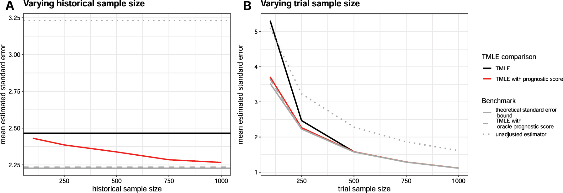
Mean estimated standard errors across estimators when historical and trial sample sizes are varied using the heterogeneous DGP. When the historical sample size is varied (Figure 1.A), the trial is fixed at n = 250. When the trial size is varied (Figure 1.B), the historical sample is fixed at
When trial sample size n and historical sample size
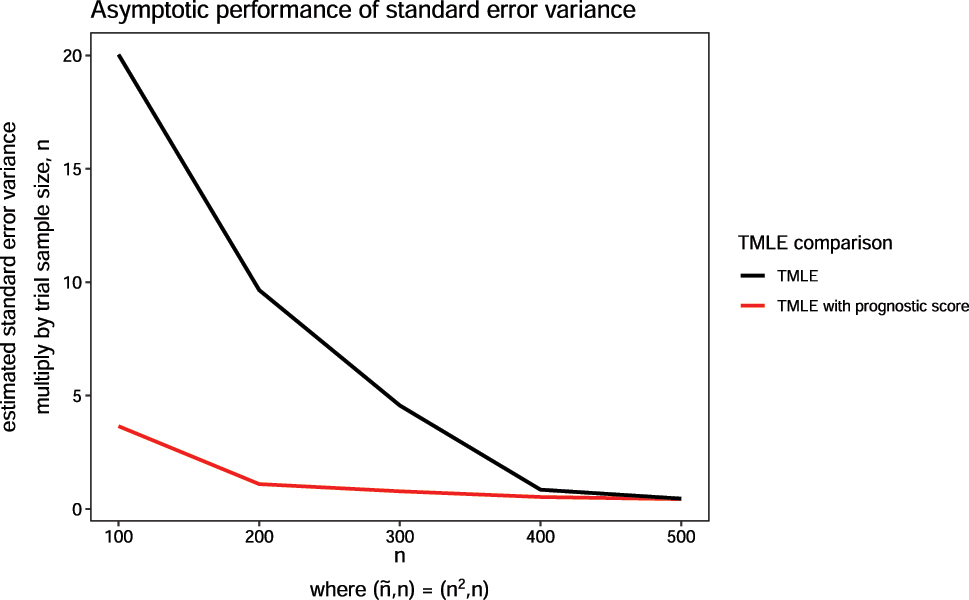
Variance of estimated standard error across estimators when historical and trial sample sizes are varied using the constant effect DGP. The historical sample size,
We also observe that our method is relatively robust to both observed and unobserved distributional shifts between historical and trial populations (Figure 3). When the shifts are large, the prognostic score may be uninformative (most evident in Figure 3.B), but including it may still improve efficiency (as seen in Figure 3.A). We also see that a good prognostic score (no shift in distribution) substantially reduces the variability of the estimated standard error. Variability increases with the magnitude of the covariate shift but still does not exceed that of TMLE without prognostic adjustment.
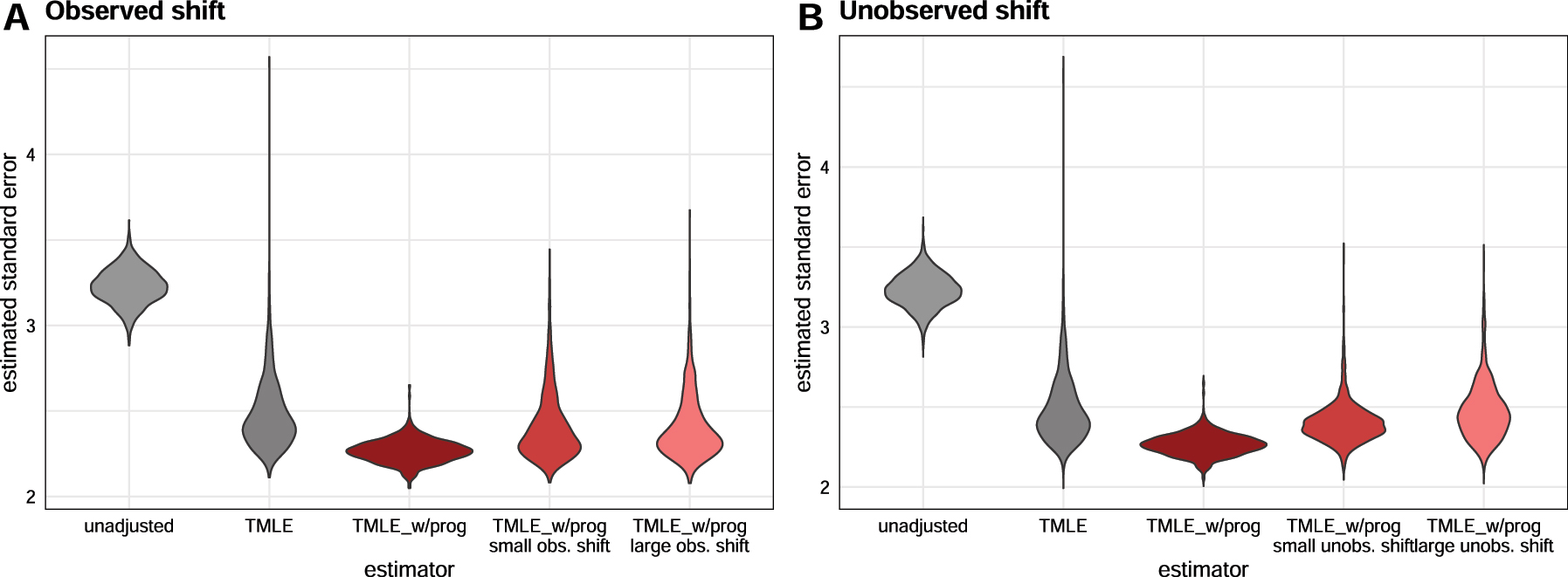
Estimated standard errors across estimators when observed (Figure 3.A) and unobserved shifts (Figure 3.B) are present in the historical sample relative to the trial sample.
5 Case study
In this section, we examine the use of TMLE with prognostic covariate adjustment in RCTs involving people diagnosed with type 2 diabetes (T2D). T2D is a chronic disease with a progressive deterioration of glucose control. Glucose control is normally evaluated by long-term blood glucose level, measured by hemoglobin A1C (HbA1C). The analyses are carried out using data provided by Novo Nordisk A/S originating from 14 previously conducted RCTs within the field of diabetes, see Supplemental Appendix E for a full overview of the trials.
We reanalyze the phase IIIb clinical trial called NN9068-4229, where the trial population consisted of insulin naive people with T2D [41]. The participants of this trial were inadequately controlled on treatment with SGLT2i, a type of oral anti-diabetic treatment (OAD). Inadequately controlled was defined as having a HbA1C of 7.0–11.0 % (both inclusive). The aim of the trial was to compare glycemic control of insulin IDegLira versus insulin IGlar as add-on therapy to SGLT2i in people with T2D. The trial was a 26-week, 1:1 randomized, active-controlled, open label, treat-to-target trial with 420 enrolled participants. One participant was excluded due to non-exposure to trial product, yielding n = 419. The efficacy of IDegLira was measured by the difference in change from baseline HbA1C to landmark visit week 26. Our corresponding historical sample came from previously conducted RCTs with a study population also consisting of insulin naive people with T2D, who were inadequately controlled on their current OADs. A total of
For the trial reanalysis in our study, we included patient measures of their demographic background, laboratory measures, concomitant medication, and vital signs. The treatment indicator where only used in the NN9068-4229 trial. For details on the specific measurements, covariate distributions, and imputation of missing covariates see Supplemental Appendix F, G, and H. For the continuous covariates we see that the mean and standard deviation are not particularly different between the historical and new trial sample, meaning that both resemble a T2D population with uncontrolled glycemic control. Furthermore we see that the range of continuous covariates for the new trial sample are contained in the range of the historical sample. This indicates that the trial population is largely similar to the historical population, at least in terms of observable covariates. For the categorical covariates the distributions vary between the historical and new trial sample. However, all the categories in the new trial sample are present in the historical sample.
A linear estimator with baseline HbA1C, region and pre-trial OADs as adjustment covariates was used in the original analysis of the primary endpoint in the NN9068-4,229 trial. In this analysis, an average treatment effect estimate of −0.340 (95 % confidence interval [−0.480; −0.200]). In this reanalysis, we report the result of five estimators: unadjusted, linear regression (adjusting for all available covariates), linear regression with a prognostic score, TMLE, and TMLE with a prognostic score. The prognostic score is explicitly defined in Supplemental Appendix I. For this application, we expanded the library of the super learner for a more comprehensive set of machine learning models than the simulation, including random forest [42], k-nearest neighbor, and a more comprehensive set of tuning parameters for the xgboost model in addition to the previously specified library, see Supplemental Appendix B. Separately, we obtained the correlation of the fitted prognostic score against the trial outcome. The prognostic score’s correlation with the outcome is 0.752 with control subjects and 0.622 with treated subjects, indicating that adjustment for the score should result in an improvement over unadjusted estimation [17].
This is a reanalyses of the NN9068-4229 trial using five different estimators where 1:1 randomization was performed. The total sample size is n = 419.
From Table 3, we see that the smallest confidence interval is obtained using TMLE with prognostic score. All methods obtain similar point estimates except from the unadjusted estimator. Notice that the linear estimator with or without a prognostic score yields the same results, since the prognostic model is a linear model in this case (chosen as the model that yielded lowest MSE from 20-fold cross-validation within the discrete super learner).
Estimates for average treatment effect (ATE) and with 95 % confidence levels of change in hemoglobin A1C (HbA1C) from baseline to week 26 for insulin IDegLira versus insulin IGlar as add-on therapy to SGLT2i in people with type 2 diabetes.
| Prognostic score | TMLE | Linear | Unadjusted |
|---|---|---|---|
| With | −0.351 (s.e. 0.145) | −0.355 (s.e. 0.157) | – |
| Without | −0.369 (s.e. 0.150) | −0.355 (s.e. 0.157) | −0.248 (0.192) |
This is a reanalyses of the NN9068-4229 trial using five different estimators where 50 participants from the control and treatment group, respectively, were chosen at random yielding a total sample size of n = 100. The random selection is done 10 times and the reported numbers are the average of the point estimates and standard error.
As illustrated by the simulation study and the asymptotic analysis in Sections 3.3 and 3.4, the relative benefit of prognostic adjustment is larger in smaller trials. To examine this result, we sub-sampled from the NN9068-4229 trial but reanalyzed with selecting 50 participants randomly from each group, resulting in n = 100. This random selection of 50 participants from each group is repeated 10 times and averaged to compute the point estimate and standard error. The average correlation of the prognostic score with the outcome was 0.790 with control subjects and 0.656 with treated subjects. We see an relatively larger reduction in the standard error estimate using TMLE with prognostic covariate adjustment compared to TMLE without in the reanalysis (Table 4).
Estimates for average treatment effect and with 95 % confidence levels of change in hemoglobin A1C from baseline to week 26 for insulin IDegLira versus insulin IGlar as add-on therapy to SGLT2i in people with type 2 diabetes.
| Prognostic score | TMLE | Linear | Unadjusted |
|---|---|---|---|
| With | −0.519 (s.e. 0.307) | −0.544 (s.e. 0.438) | – |
| Without | −0.582 (s.e. 0.349) | −0.544 (s.e. 0.438) | −0.344 (0.399) |
6 Discussion
In this study we demonstrate the utility of incorporating historical data via a prognostic score in an efficient estimator while maintaining strict type I error control. Using the prognostic score via covariate adjustment overall improves the performance of the efficient estimator by decreasing the standard error and improving its estimation. This method is most useful in randomized trials with small sample sizes. Our proposed method is shown to be robust against bias even when the historical sample is drawn from a different population.
Prognostic adjustment requires no assumptions to continue to guarantee unbiased causal effect estimates. However, this comes with a trade-off: without introducing the risk of bias, there is a limit on how much power can be gained and in what scenarios. For example, the method of Li et al. [13] (which imposes an additional assumption) can asymptotically benefit from the addition of historical data, whereas our method can only provide gains in small samples [13]. However, these gains are most important precisely in small samples because estimated effects are likely to be of borderline significance, whereas effects are more likely to be clear in very large samples regardless of the estimator used.
Besides being assumption-free, our method has other practical advantages relative to data fusion approaches. For one, we do not require a single, well-defined treatment in the historical data. Moreover, we do not require an exact overlap of the covariates measured in the historical and trial data sets. This means trial data can have more measured covariates compared to the historical data, but the prognostic score could only be derived from the overlapping measured covariate set. For multiple historical data sets, there is no need to manually select one over another. It is easy to utilize the data sets: if they are believed to be drawn from substantially different populations, separate prognostic scores can be built from each of them and included as covariates in the trial analysis. Additional variable selection procedure (screening) can be performed within the Super Learner specification. As long as one of these scores is a good approximation of the outcome-covariate relationship in one or more arms of the trial, there will be added benefits to power.
Prognostic adjustment with efficient estimators can also be used with pre-built or public prognostic models: the analyst does not need direct access to the historical data if they can query a model for predictions. This is helpful in cases where data is “federated” and cannot move (e.g. when privacy must be protected or data has commercial value).
Our approach is closely related to the transfer learning literature in machine learning. In transfer learning, the goal is to use a (large) “source” dataset to improve prediction for a “target” population for which we have only minimal training data [43], [44], [45]. In this work we use a particular method of “transfer” (adjusting for the source/historical model prediction) to improve the target (trial) predictions, which drives variance reduction. It should also be possible to leverage other more direct forms of model transfer for the outcome regression, such as pre-training a deep learning model on the historical data and then fine-tuning using the trial data.
The theory we developed to explain the benefits of prognostic adjustment in the context of efficient estimation for trials is easily generalizable to estimation of any kind of pathwise differentiable parameter augmented with transfer learning from an auxiliary dataset. The specific breakdown of different terms may differ but the overall intuition should be the same: transfer learning may accelerate the disappearance of higher-order terms that depend on the error rates of regression estimates.
Lastly, since we use efficient estimators, we can leverage the results of Schuler [27] to prospectively calculate power with prognostic adjustment [27]. In fact, we suspect the methods of power calculation described in that work would improve in accuracy with prognostic adjustment since the outcome regressions are “jump-started” with the prognostic score. Verification of this fact and empirical demonstration will be left to future work.
Funding source: Innovationsfonden
Award Identifier / Grant number: 2052-00044B
Funding source: National Science Foundation
Award Identifier / Grant number: DGE 2146752
Funding source: Bill and Melinda Gates Foundation
Award Identifier / Grant number: OPP1165144
Supporting information
The following supporting information is available as part of the online article:
Appendix A. Expectation calculation when incorporating unobserved covariate.
Appendix B. Discrete super learner specifications for simulation and case study.
Appendix C. Simulation results for different data generation processes.
Appendix D. Empirical standard error estimates.
Appendix E. Case study data summary.
Appendix F. Summary of continuous measurements of the baseline.
Appendix G. Summary of categorical measurements of the baseline.
Appendix H. Missing pattern of the case study.
Appendix I. Case study prognostic score.
Acknowledgments
The authors would like to thank study participants and staff for their contributions. This research was conducted on the Savio computational cluster resource provided by the Berkeley Research Computing program at the University of California, Berkeley. This computing resource was supported by the UC Berkeley Chancellor, Vice Chancellor for Research, and Chief Information Officer. The authors thank Christopher Paciorek for answering Savio related inquiries. This research was also conducted on Kaiser Permanente advance computing infrastructure platform. The authors thank Woodward B Galbraith and Tejomay Gadgil for their technical support on shortening the simulation computation time.
-
Research ethics: Not applicable.
-
Informed consent:Not applicable.
-
Author contributions: LDL and AS conceptualized the methodology of this research. LDL wrote the original draft and conducted the investigation, formal analysis, and visualizations. LDL worked closely together with AEH and AS on the research framework and discussion. EH-F collaborated with LDL on the application of the research and ran case study analysis. EH-F wrote the original draft of the updated case study analysis section and result section. EH-F also was involved in simulation discussion with LL and AS. All authors contributed significantly to the review and editing of the paper. The authors have accepted responsibility for the entire content of this manuscript and approved its submission.
-
Use of Large Language Models, AI and Machine Learning Tools: None declared.
-
Conflict of interest: Alan E. Hubbard is a co-editors-in-chief of IJB. None of the authors, including Alan E. Hubbard, had a role in the peer review or handling of this manuscript. All other authors state no conflict of interest.
-
Research funding: This research was made possible by funding from the National Science Foundation (DGE 2146752) to LDL and global development grant (OPP1165144) from the Bill & Melinda Gates Foundation for AEH to the University of California, Berkeley, CA, USA. This research also received funding from Innovation Fund Denmark (Grant number 2052-00044B) for EFD to Novo Nordisk A/S. The funders had no role in study design, data collection and analysis, decision to publish, or preparation of the manuscript.
-
Data availability: Not applicable.
References
1. Bentley, C, Cressman, S, van der Hoek, K, Arts, K, Dancey, J, Peacock, S. Conducting clinical trials – costs, impacts, and the value of clinical trials networks: a scoping review. Clin Trials 2019;16:183–93. https://doi.org/10.1177/1740774518820060.Search in Google Scholar PubMed
2. Glennerster, R. Chapter 5 – the practicalities of running randomized evaluations: partnerships, measurement, ethics, and transparency. In: Banerjee, AV, Duflo, E, editors. Handbook of economic field experiments. Oxford: Elsevier; 2017, vol 1:175–243 pp.10.1016/bs.hefe.2016.10.002Search in Google Scholar
3. Temple, R, Ellenberg, SS. Placebo-controlled trials and active-control trials in the evaluation of new treatments. Part 1: ethical and scientific issues. Ann Intern Med 2000;133:455–63. https://doi.org/10.7326/0003-4819-133-6-200009190-00014.Search in Google Scholar PubMed
4. Wu, P, Luo, S, Geng, Z. On the comparative analysis of average treatment effects estimation via data combination. J Am Stat Assoc 2025;1–12. https://doi.org/10.1080/01621459.2024.2435656.Search in Google Scholar
5. Bareinboim, E, Pearl, J. Causal inference and the data-fusion problem. Proc Natl Acad Sci USA 2016;113:7345–52. https://doi.org/10.1073/pnas.1510507113.Search in Google Scholar PubMed PubMed Central
6. Shi, X, Pan, Z, Miao, W. Data integration in causal inference. Wiley Interdiscip Rev Comput Stat 2023;15. https://doi.org/10.1002/wics.1581.Search in Google Scholar PubMed PubMed Central
7. Colnet, B, Mayer, I, Chen, G, Dieng, A, Li, R, Varoquaux, G, et al.. Causal inference methods for combining randomized trials and observational studies: a review. Stat Sci 2024;39:165–91. https://doi.org/10.1214/23-STS889.Search in Google Scholar
8. Hill, JL. Bayesian nonparametric modeling for causal inference. J Comput Graph Stat 2011;20:217–40. https://doi.org/10.1198/jcgs.2010.08162.Search in Google Scholar
9. Li, F, Ding, P, Mealli, F. Bayesian causal inference: a critical review. Philos Trans A Math Phys Eng Sci 2023;381:20220153. https://doi.org/10.1098/rsta.2022.0153.Search in Google Scholar PubMed
10. Huang, M, Egami, N, Hartman, E, Miratrix, L. Leveraging population outcomes to improve the generalization of experimental results: application to the JTPA study. Ann Appl Stat 2023;17:2139–64. https://doi.org/10.1214/22-AOAS1712.Search in Google Scholar
11. Degtiar, I, Rose, S. A review of generalizability and transportability. Annu Rev Stat Appl. 2023;10:501–24. https://doi.org/10.1146/annurev-statistics-042522-103837.Search in Google Scholar
12. Lee, D, Yang, S, Dong, L, Wang, X, Zeng, D, Cai, J. Improving trial generalizability using observational studies. Biometrics 2021;1213–25. https://doi.org/10.1111/biom.13609.Search in Google Scholar PubMed PubMed Central
13. Li, X, Miao, W, Lu, F, Zhou, XH. Improving efficiency of inference in clinical trials with external control data. Biometrics 2023;79:394–403. https://doi.org/10.1111/biom.13583.Search in Google Scholar PubMed
14. Dang, LE, Tarp, JM, Abrahamsen, TJ, Kvist, K, Buse, JB, Petersen, M, et al.. A cross-validated targeted maximum likelihood estimator for data-adaptive experiment selection applied to the augmentation of RCT control arms with external data. arXiv preprint 2022. https://doi.org/10.48550/arXiv.2210.05802.Search in Google Scholar
15. FDA. Adjusting for covariates in randomized clinical trials for drugs and biological products. Internet: Center for Drug Evaluation and Research, Center for Biologics Evaluation and Research; 2023.Search in Google Scholar
16. Van Lancker, K, Bretz, F, Dukes, O. The use of covariate adjustment in randomized controlled trials: an overview. arXiv preprint 2023. https://doi.org/10.48550/arXiv.2306.05823.Search in Google Scholar
17. Schuler, A, Walsh, D, Hall, D, Walsh, J, Fisher, C, for the Critical Path for Alzheimer’s Disease; the Alzheimer’s Disease Neuroimaging Initiative; the Alzheimer’s Disease Cooperative Study. Increasing the efficiency of randomized trial estimates via linear adjustment for a prognostic score. Int J Biostat 2022;18:329–56. https://doi.org/10.1515/ijb-2021-0072.Search in Google Scholar PubMed
18. Holzhauer, B, Adewuyi, ET. “Super-covariates”: using predicted control group outcome as a covariate in randomized clinical trials. Pharm Stat 2023;22:1062–75. https://doi.org/10.1002/pst.2329.Search in Google Scholar PubMed
19. Van Der Laan, MJ, Rubin, D. Targeted maximum likelihood learning. Int J Biostat 2006. https://doi.org/10.2202/1557-4679.1043.Search in Google Scholar
20. Van der Laan, MJ, Rose, S. Targeted learning: causal inference for observational and experimental data. New York: Springer; 2011, 4.10.1007/978-1-4419-9782-1Search in Google Scholar
21. Diaz, I. Machine learning in the estimation of causal effects: targeted minimum loss-based estimation and double/debiased machine learning. Biostatistics 2020;21:353–8. https://doi.org/10.1093/biostatistics/kxz042.Search in Google Scholar PubMed
22. Glynn, AN, Quinn, KM. An introduction to the augmented inverse propensity weighted estimator. Polit Anal 2010;18:36–56. https://doi.org/10.1093/pan/mpp036.Search in Google Scholar
23. Chernozhukov, V, Chetverikov, D, Demirer, M, Duflo, E, Hansen, C, Newey, W, et al.. Double/debiased machine learning for treatment and structural parameters. Econom J 2018;21:C1–68. https://doi.org/10.1111/ectj.12097.Search in Google Scholar
24. Rosenblum, M, van der Laan, MJ. Simple, efficient estimators of treatment effects in randomized trials using generalized linear models to leverage baseline variables. Int J Biostat 2010;6:13. https://doi.org/10.2202/1557-4679.1138.Search in Google Scholar PubMed PubMed Central
25. Petersen, ML, van der Laan, MJ. Causal models and learning from data: integrating causal modeling and statistical estimation. Epidemiology 2014;25:418–26. https://doi.org/10.1097/ede.0000000000000078.Search in Google Scholar PubMed PubMed Central
26. Hansen, BB. The prognostic analogue of the propensity score. Biometrika 2008;95:481–8. https://doi.org/10.1093/biomet/asn004.Search in Google Scholar
27. Schuler, A. Designing efficient randomized trials: power and sample size calculation when using semiparametric efficient estimators. Int J Biostat 2021;18:151–71. https://doi.org/10.1515/ijb-2021-0039.Search in Google Scholar PubMed
28. van der Laan, MJ, Polley, EC, Hubbard, AE. Super learner. Stat Appl Genet Mol Biol 2007;6:25. https://doi.org/10.2202/1544-6115.1309.Search in Google Scholar PubMed
29. Polley, EC, van der Laan, MJ. Super learner in prediction. U.C. Berkeley Division of Biostatistics Working Paper Series 2010; Working Paper 266. https://biostats.bepress.com/ucbbiostat/paper266.Search in Google Scholar
30. Rothe C. Flexible covariate adjustments in randomized experiments; 2018. Available from: https://madoc.bib.uni-mannheim.de/52249/.Search in Google Scholar
31. Moore, KL, van der Laan, MJ. Covariate adjustment in randomized trials with binary outcomes: targeted maximum likelihood estimation. Stat Med 2009;28:39–64. https://doi.org/10.1002/sim.3445.Search in Google Scholar PubMed PubMed Central
32. Schuler, A, van der Laan, M. Introduction to modern causal inference. 2022. https://alejandroschuler.github.io/mci [Accessed 9 12 2023].Search in Google Scholar
33. Kennedy, EH. Semiparametric doubly robust targeted double machine learning: a review. In: Handbook of statistical methods for precision medicine. Boca Raton, FL: Chapman & Hall; 2024: 207–36 pp. https://doi.org/10.48550/arXiv.2203.06469.Search in Google Scholar
34. Hahn, J. On the role of the propensity score in efficient semiparametric estimation of average treatment effects. Econometrica 1998:315–31. https://doi.org/10.2307/2998560.Search in Google Scholar
35. Chakrabortty, A, Dai, G, Tchetgen, ET. A general framework for treatment effect estimation in semi-supervised and high dimensional settings. arXiv preprint 2022. https://doi.org/10.48550/arXiv.2201.00468.Search in Google Scholar
36. White, H. A heteroskedasticity-consistent covariance matrix estimator and a direct test for heteroskedasticity. Econometrica 1980;48:817–38. https://doi.org/10.2307/1912934.Search in Google Scholar
37. MacKinnon, JG, White, H. Some heteroskedasticity-consistent covariance matrix estimators with improved finite sample properties. J Econom 1985;29:305–25. https://doi.org/10.1016/0304-4076(85)90158-7.Search in Google Scholar
38. Long, JS, Ervin, LH. Using heteroscedasticity consistent standard errors in the linear regression model. Am Statistician 2000;54:217–24. https://doi.org/10.1080/00031305.2000.10474549.Search in Google Scholar
39. Chen, T, Guestrin, C. XGBoost: a scalable tree boosting system. In: Proceedings of the 22nd ACM SIGKDD international conference on knowledge discovery and data mining. KDD ’16. New York, NY, USA: Association for Computing Machinery; 2016:785–94 pp.10.1145/2939672.2939785Search in Google Scholar
40. Friedman, JH. Multivariate adaptive regression Splines. aos 1991;19:1–67. https://doi.org/10.1214/aos/1176347963.Search in Google Scholar
41. gov, C. A clinical trial comparing glycaemic control and safety of insulin degludec/liraglutide (IDegLira) versus insulin glargine (IGlar) as add-on therapy to SGLT2i in subjects with type 2 diabetes mellitus (DUAL TM IX). 2020. Available from: https://clinicaltrials.gov/study/NCT02773368?cond=DUALTMAccessed:2023-9-25.Search in Google Scholar
42. Breiman, L. Random forests. Mach Learn 2001;45:5–32.10.1023/A:1010933404324Search in Google Scholar
43. Torrey, L, Shavlik, J. Transfer learning. In: Handbook of research on machine learning applications and trends: algorithms, methods, and techniques. Hershey, PA: IGI Global; 2010:242–64 pp.10.4018/978-1-60566-766-9.ch011Search in Google Scholar
44. Zhuang, F, Qi, Z, Duan, K, Xi, D, Zhu, Y, Zhu, H, et al.. A comprehensive survey on transfer learning. Proc IEEE 2021;109:43–76. https://doi.org/10.1109/jproc.2020.3004555.Search in Google Scholar
45. Weiss, K, Khoshgoftaar, TM, Wang, D. A survey of transfer learning. J Big Data 2016;3:1–40. https://doi.org/10.1186/s40537-016-0043-6.Search in Google Scholar
Supplementary Material
This article contains supplementary material (https://doi.org/10.1515/ijb-2024-0018).
© 2025 Walter de Gruyter GmbH, Berlin/Boston
Articles in the same Issue
- Frontmatter
- Research Articles
- Prognostic adjustment with efficient estimators to unbiasedly leverage historical data in randomized trials
- Homogeneity test and sample size of response rates for AC 1 in a stratified evaluation design
- A review of survival stacking: a method to cast survival regression analysis as a classification problem
- DsubCox: a fast subsampling algorithm for Cox model with distributed and massive survival data
- A hybrid hazard-based model using two-piece distributions
- Regression analysis of clustered current status data with informative cluster size under a transformed survival model
- Bayesian covariance regression in functional data analysis with applications to functional brain imaging
- Risk estimation and boundary detection in Bayesian disease mapping
- An improved estimator of the logarithmic odds ratio for small sample sizes using a Bayesian approach
- Short Communication
- A multivariate Bayesian learning approach for improved detection of doping in athletes using urinary steroid profiles
- Research Articles
- Guidance on individualized treatment rule estimation in high dimensions
- Weighted Euclidean balancing for a matrix exposure in estimating causal effect
- Penalized regression splines in Mixture Density Networks