Bayesian Autoregressive Frailty Models for Inference in Recurrent Events
-
Marta Tallarita

 ,
Maria De Iorio
,
Maria De Iorio

Abstract
We propose autoregressive Bayesian semi-parametric models for gap times between recurrent events. The aim is two-fold: inference on the effect of possibly time-varying covariates on the gap times and clustering of individuals based on the time trajectory of the recurrent event. Time-dependency between gap times is taken into account through the specification of an autoregressive component for the frailty parameters influencing the response at different times. The order of the autoregression may be assumed unknown and is an object of inference. We consider two alternative approaches to perform model selection under this scenario. Covariates may be easily included in the regression framework and censoring and missing data are easily accounted for. As the proposed methodologies lie within the class of Dirichlet process mixtures, posterior inference can be performed through efficient MCMC algorithms. We illustrate the approach through simulations and medical applications involving recurrent hospitalizations of cancer patients and successive urinary tract infections.
1 Introduction
Recurrent event processes generate events repeatedly over time and recurrent event data arise in many applications, for example in medicine (e. g. [1, 2]), economy (e. g. [3]) and technology (for example, [4]). Typical examples include recurrent infections, asthma attacks, hospitalizations, product repairs and machine failures. In particular, in this work, we are interested in settings where recurrent event processes are available from a large number of individuals, but with a small number of occurrences for each subject. Here we consider a benchmark dataset, in which we are interested in modelling the time between re-hospitalisation after surgery in colon cancer patients, and an application where the main clinical outcome is recurrence of urinary tract infections.
Typically, the focus is on modeling the rate of occurrence, accounting for the variation within and between individuals. Moreover, in applications, it is often of interest to assess the relationship between event occurrence and potential explanatory factors. The two main statistical approaches to perform inference on recurrent event data are (see [5]): (i) modelling the intensity function of the event counts {N(t), t ≥ 0}, where N(t) is the number of events between the time origin and time t; (ii) modelling the whole sequence of gap times between successive realizations of the recurrent events.
The first approach is most suitable when individuals frequently experience the event of interest and the occurrence does not alter the process itself. The canonical framework for the analysis of event counts is the Poisson process. For a full review of this class of methods, see [6]. Wang et al. [7] suggest a subject-specific nonstationary Poisson process via a latent variable to model the occurrence of recurrent events. An alternative method was introduced by Thall [8] who considers a parametric mixed Poisson model which deals with covariates. Further, [9] propose a semiparametric model based on a non-homogeneous Poisson process. Finally, Pepe and Cai [10], Lawless and Nadeau [11] and Lawless et al. [12] propose semiparametric procedures for making inferences about the mean and rate functions of the counting process without the Poisson-type assumption.
The second approach based on gap times is more appropriate when the events are relatively infrequent, when, after an event, individual renewal takes place in some way, or when the focus of the analysis is the prediction of the time to the next event. The two dominant families of models in this framework are accelerated failure time (AFT) and proportional hazards (PH) regressions. For example, Prentice et al. [13] propose a PH model for recurrent events, while Chang and Wang [14] propose a slightly different model by incorporating two kinds of covariates: some structural covariates (fixed) and some episode-specific covariates. Frailty models are discussed in McGilchrist and Aisbett [15] and Duchateau and Janssen [16]. However, in the frailty models time dependence is not modelled, but in many situations the occurrence of a past event may change the risk of a later event and so it is essential to incorporate and quantify how the occurrence of a past event may change the risk of a later event. Lin et al. [17] overcome this problem and propose a Bayesian recurrent event model to account for both subject-specific heterogeneity and event dependence. An alternative approach to frailty models consists in specifying a multivariate distribution for the gap times using copulas (see, for example, [18, 19]). This strategy requires specifying the marginal distribution of each gap time and then using a copula to introduce dependence.
1.1 Bayesian nonparametric framework
This paper lies within the gap times approach and develops a Bayesian semiparametric model for gap times between events. We assume that the joint distribution of the finite sequence of gap times for each individual is the product of the conditional distributions of each gap time, given the previous ones. Moreover, we specify a regression model for each of these conditional distributions to link the realization of each gap time to possibly time-varying covariates and previous gap times. To account for inter-subject variability, we introduce individual specific frailty parameters which we model flexibly using a Dirichlet process mixture prior as random effects distribution. Dirichlet process mixture (DPM) models [20, 21] are arguably the most common nonparametric Bayesian prior and have proved successful in many applications due to their flexibility and ease of computation. DPM models are mixtures of a parametric distribution where the mixing measure is the Dirichlet process (DP) introduced by Ferguson [22]. It is well known that the DP is almost surely discrete, and that if G is a DP(M, G0) with total mass parameter M and baseline distribution G0, then G admits the following representation [23]:
where δθ is a point-mass at θ, the weights follow a stick-breaking process,
Due to the discreteness of G, the DPM prior induces clustering of the subjects in the sample based on the trajectory of the recurrent events over time, where the number K of clusters is unknown and learned from the data. Earliest examples of the use of a Bayesian nonparametric distribution for the random effects can be found in Müller and Rosner [24] and Kleinman and Ibrahim [25]. More recently, Pennell and Dunson [26] employ a Dirichlet process prior to build semiparametric dynamic frailty models for multiple event time data, allowing also the frailty parameter to change over time. Moreover, Paulon et al. [27] develop a joint model for gap times between two consecutive hospitalizations and survival time using the DP as random effect distribution, but do not explicitly account for the temporal dependence between gap times observed on the same individual.
In this work, we investigate different strategies to link gap times at time t with previous gap times. We start by assuming a standard Markov model where also the order of dependence p is unknown and is object of inference. We explore two different strategies to specify a prior distribution on p: one involves eliciting a prior directly on the space of all possible Markov models for p ∈ {0, 1, …, P}, while the other approach employs spike and slab base measures and it is in the spirit of stochastic search variable selection [28]. In conclusion, the main contribution of this work is to provide, within a Bayesian nonparametric framework, a model for gap times which accommodates for temporal dependence, performs variable selection on the order of dependence with two different approaches, allows for clustering of individuals and inter-subject variability, is able to handle different numbers of gap times per individual and missingness.
In Section 2 we introduce the model, while in Section 3 we explain how to perform inference on the order of dependence in the Markov structure. In Section 4 we investigate the performance of the proposed approach in simulations and compare the different strategies to model time dependency and to select the order p. Sections 5 and 6 present two medical applications involving recurrent hospitalizations and urinary tract infections, respectively. We conclude the paper in Section 7.
2 Autoregressive frailty models via Dirichlet process mixtures
We consider data on N individuals. We assume that 0: = Ti0 corresponds to the start of the event process and that individual i is observed over the time interval [0, τi]. If ni events are observed at times
where
The likelihood for all the sample is then given by:
where
The vector
2.1 Nonparametric AR(1)-type models
Following a similar modelling strategy to the one described in Di Lucca et al. [29], a straightforward way to introduce dependence among random effects at different times is to allow the distribution of αij to depend on some summary of the observations up to time j – 1:
When j = 1, the distribution of the random effect αi1 simplifies as the autoregressive term in (2) disappears and it reduces to the Normal distribution with mean mi0.
We assume conditional independence among subjects, given the parameters, and that
assuming a priori independence among the different parameters.
When implementing the model in JAGS, we opt for marginal uniform priors on bounded interval for σ2 and τ2 as suggested by. Gelman [30] as inverse-gamma distributions give numerical instability problems when hyperparameters are small. Moreover, Gelman [30] recommends uniform distributions (on bounded intervals) for scale parameters in hierarchical models as being weakly-informative, opposite to inverse-gamma priors for variance parameters, which are very sensitive to the choice of the hyperparameters themselves.
The choice of g in (2) is obviously crucial and depends on the context and the goals of the inference problem. Common choices in the literature are:
Note that, when
2.2 Nonparametric AR(p) models
The model in Section 2.1 can be extended to include higher order dependence, by modifying (2) – (3) as follows:
The distribution of αij for j ≤ p, depends only on the available past observations as in any AR(p) model. Prior specification for the remaining parameters is the same as described in Section 2.1.
3 Estimating the order of dependence
In (5) we assume that the order of dependence on past observations is a fixed integer p. However, this parameter is often unknown in applications, and it needs to be estimated. A wealth of research focuses on Bayesian model selection (see, for example, [31, 32]). Here we concentrate on two approaches. The first one modifies the base measure of the DP by including a spike and slab distribution on the autoregressive coefficient, leading to the Spiked Dirichlet process prior introduced by Kim et al. [33]. The second one involves the direct specification of a prior on p, and then, conditional on p, we specify the prior distribution for the remaining parameters; in this case the dimension of the parameter vector
3.1 Spike and slab base measure
Kim et al. [33] introduce the Spiked Dirichlet process prior in the context of regression. A key feature of their method is to employ the spike and slab distribution, i. e. a mixture of a point mass at 0 and a continuous distribution as centering distribution of the DP. This implies that, in a regression context, some coefficients have a positive probability of being equal to 0 and therefore they are not influential on the response of interest. Their technique is easily accommodated in our context by simply modifying G0 in (7) as
where the introduction of hyperpriors on the weights of the mixture induces sparsity.
3.2 Prior on the Order of Dependence
Following Quintana and Müller [34], we specify a prior directly on the order p of the autoregressive process and then, conditioning on p, we set a Dirichlet Process prior of appropriate dimension for the parameters of the AR(p), i. e. the vector
When p = 0, the process simplifies as the autoregressive term in (9) disappears and the base measure of the DP reduces to the Normal distribution for the intercept term.
An MCMC algorithm to perform posterior inference on the order of dependence is described in [34], who sample from the posterior distribution of p given the data. For the JAGS implementation we have opted for a pseudo-prior approach, see [35].
4 Simulated data
In order to check the performance of the class of models proposed in the previous sections, different simulation scenarios have been created. The simulated datasets discussed in this section, as well as the scenario in Section 3 of Supplementary Material, are generated from a mixture of Gaussian distributions. In Section 4 of Supplementary Material, results from a simulation scenario where data are generated from a mixture of Exponential distributions are presented. For all scenarios we generate data without censoring and datasets in which the subjects are right-censored with respect to their last gap time. Posterior inference for these examples, as well as for the real data applications in Section 5 and 6, can be performed through a standard Gibbs sampler algorithm, which we implement in JAGS [36], using a truncation-based algorithm for stick-breaking priors [37]. For all simulations, we run the algorithm for 251,000 iterations, discarding the first 1,000 iterations as burn-in and thinning every 50 iterations to reduce the autocorrelation of the Markov chain. The final sample size is then 5,000. The computational time for both simulation scenarios was close to three hours using a MacBook Pro with 2, 4 GHz Intel Core i5 processor type. Unless otherwise stated, we check through standard diagnostics criteria such as those available in the R package CODA [38] that convergence of the chain is satisfactory for most of the parameters.
4.1 Simulation scenario 1
We consider a simulated dataset of N = 300 subjects, with ni randomly generated from a Poisson distribution. In particular we select ni in such a way that all subjects have at least three gap times:
while another third is generated from
and the last 100 observations are generated from
In simulating the data, we assume independence across subjects. In this example, for ease of explanation, we do not include covariates. We introduce censoring according to the following procedure. Firstly, we set the percentage of the sample for which we have censoring. In this simulation we have used three different censoring rates: 10 %, 25 % and 50 %. We consider at least two gap times for each individual and so for all patients i with censoring we generate a censoring time Ci from a Uniform distribution defined on the interval
We fit the model (1), (5)–(6) with p = 3:
where G0 is given by the product of spike and slab distributions as defined in (8):
In fitting the model we set:
Hyperparameters are chosen in order to specify vague marginal prior distributions. Figure 1 shows the predictive distributions of mi0, mi1, mi2 and mi3 obtained with the spike and slab base measures. Red, blue, green and grey lines correspond to estimates obtained using the dataset with 0 %, 10 %, 25 % and 50 % censoring rates, respectively. By visual inspection, it is clear that the marginal posterior predictive distributions of the mij’s agree with the true values used to generate the dataset. In fact, the predictive distribution of mi0 is concentrated around 0, while the predictive distributions of mi1, mi2 and of mi3 are bimodal. Furthermore, the variance of the predictive distributions of each mij becomes larger with increasing censoring rate, because we have less information about the population parameters. The marginal posterior distributions of η1, η2, and η3 in the prior (8), not reported here, concentrate most mass on 1.
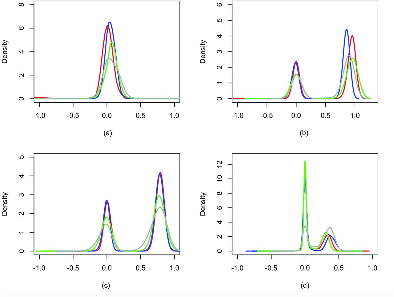
Simulation scenario 1: predictive marginal distributions of mi0 (a), mi1 (b), mi2 (c) and mi3 (d) under the spike and slab prior. Red, blue, green and grey lines correspond to estimates obtained using the dataset with 0 %, 10 %, 25 % and 50 % censoring rates, respectively.
Moreover, there is a clear difference between the posterior distribution of K, the number of distinct components in the mixture (5)–(6), using the data with and without censoring (results shown in Figure 2 of Supplementary Material). Using data without censoring, the configuration involving K = 3 clusters has the highest posterior probability: posterior inference on K is in agreement with the 3 components used to generate the data. Instead, using data with censoring, the number of clusters increases as the model needs to accommodate for the lack of information and the greater uncertainty in the distribution of the gap times. We also fit model (1), (9) to this dataset and similar results are obtained using the prior on the order of dependence. For further details, see Section 1 and Figure 1 of Supplementary Material.
4.2 Simulation Scenario 2
In this section we simulate a dataset of N = 200, with ni randomly generated from a Poisson distribution. Similarly as in the previous example, we select
while the other half is independently generated from
As in the previous example, covariates are not included and we introduce censoring using the same strategy. Also in this case we set the censoring rate equal to 10 %, 25 % and 50 %. We consider at least two gap times for each individual and for all the patients with censoring we generate a censoring time Ci from a Uniform distribution defined on the interval
Also for this scenario, we fit both model (1), (5)–(6), (8) and model (1), (9). Here we report posterior inference of the latter model, with the prior on the order of dependence, where the maximum order of dependence is P = 3 and the prior hyperparameters (corresponding to a vague prior) are set as follows:
The mode of the marginal posterior distribution of p is 2 for all datasets without and with censoring, with corresponding posterior probability reported in the Table 1. In particular, the mass placed on p = 2 decreases with increasing censoring rate.
Simulation scenario 2: posterior distributions (masses) of p under the prior on the order of dependence for different rates of censoring.
| Censoring rate | p = 0 | p = 1 | p = 2 | p = 3 |
|---|---|---|---|---|
| 0 % | 0.01 | 0.01 | 0.98 | 0.00 |
| 10 % | 0.18 | 0.01 | 0.81 | 0.00 |
| 25 % | 0.21 | 0.02 | 0.77 | 0.00 |
| 50 % | 0.25 | 0.02 | 0.73 | 0.00 |
Conditional on p = 2, Figure 2 reports the predictive distributions of mi0, mi1 and mi2. Red, blue, green and grey lines correspond to estimates obtained using the dataset with censoring rates equal to 0 %, 10 %, 25 % and 50 %, respectively.
More in detail, the predictive distribution of mi0 is concentrated around 0, while the predictive distributions of mi1 and of mi2 are bimodal with mode around {–0.9, 0.9} and {–0.7, 0.7}, respectively. Also in this scenario, the variance of the predictive distributions of mij becomes larger with increasing censoring rate.
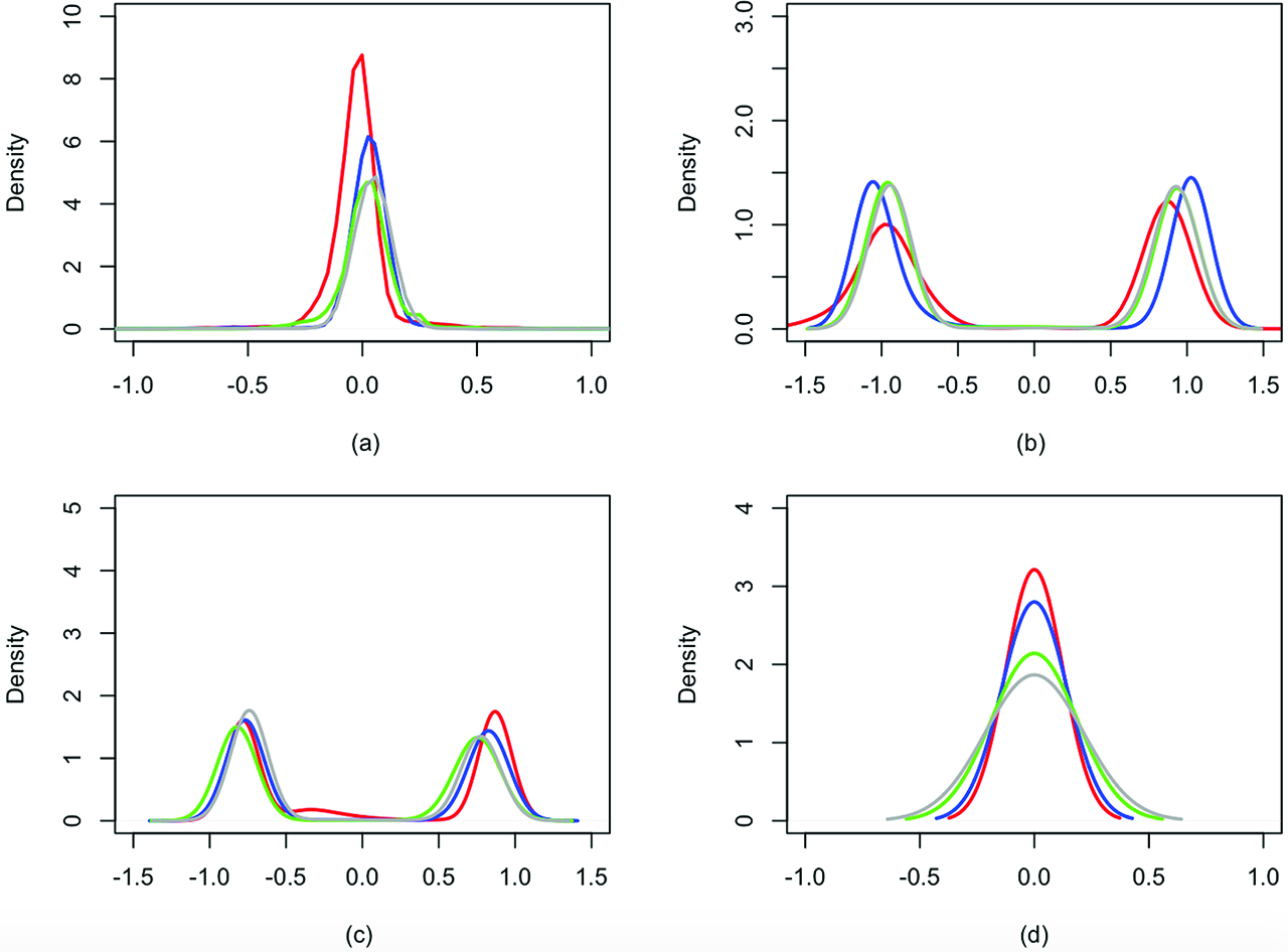
Simulation scenario 2: predictive marginal distributions of mi0 (a), mi1 (b), mi2 (c) and mi3 (d) under the prior on the order of dependence, conditioning on p = 2. Red, blue, green and grey lines correspond to estimates obtained using the dataset with 0 %, 10 %, 25 % and 50 % censoring rates, respectively.
Finally, in the dataset without censoring time, conditioning on p = 2, the posterior mode for the number K of clusters is 2 (results not shown), with associated posterior probability equal to 0.5, while for the datasets with censoring, the number of clusters increases because of the greater uncertainty on the distribution of gap times. See Section 2 of Supplementary Material for the results obtained by fitting the model with the spike and slab base measure.
To evaluate the computational performance of the two approaches for model selection, we report in Table 2 summary statistics for the Effective Sample Size (ESS). ESS measures the amount by which autocorrelation within a MCMC chain increases uncertainty in estimates. The ESS of a parameter aims to estimate how many iid samples have the same estimation performance as the correlated samples found in the MCMC chain and it will be typically smaller than the final sample size. Hence large values of the ESS denote smaller autocorrelation in the chains; for further details, see [39]. Summary statistics are evaluated across the ESS of all estimated parameters. We report results for both simulations scenarios and four different censoring rates. The empirical distributions of the ESS in Table 2 seem comparable across different prior specifications and scenarios.
ESS: summary statistics. We report 2.5 %, 50 %, 97.5 % empirical quantiles of the ESS evaluated for all estimated parameters. SS denotes the spike and slab base measure, while POD indicates the prior on the order of dependence.
| Method | Censoring rate | Scenario 1 | Scenario 2 |
|---|---|---|---|
| SS | 0 % | (37.45, 104.40, 245.09) | (38.96, 80.780, 207.70) |
| 10 % | (57.57, 144.70, 345.70) | (101.96, 120.78, 296.70) | |
| 25 % | (43.50, 111.50, 241.80) | (167.96, 225.78, 370.70) | |
| 50 % | (698.60, 1235.00, 1865.00) | (174.67, 253.82, 390.70) | |
| POD | 0 % | (41.52, 114.80, 265.09) | (143.30, 519.70, 573.00) |
| 10 % | (47.79, 141.01, 351.04) | (165.92, 290.60, 589.20) | |
| 25 % | (53.50, 131.09, 298.09) | (821.90, 2125.00, 4521.00) | |
| 50 % | (398.06, 1565.00, 1951.20) | (812.99, 2245.30, 4728.55) | |
4.3 Comparison with the time-dependent frailty model
In this subsection, we compare our model with the time-dependent frailty model of [40] on the same simulated data described in the previous section. This strategy not only accounts for dependence of recurrent failure times within observations for the same subject by introducing a subject-specific random frailty, but also for the order of events, which is a significant feature of dependence. In this setup, time independence is introduced in the model for the intensity function of the recurrent event process at time t:
where the variable ci(t) is the censoring indicator equal to 1 if patient i is observed at time t and 0 otherwise. The function λ0(t) is an unspecified baseline intensity, while Vi(t) is a subject-specific random frailty capturing the risk not accounted for by potential risk variables included in the analysis. The model can be extended to include time-dependent covariates. Following [40] we assume
where
Also for this model posterior inference can be performed through a standard Gibbs sampler algorithm, which we implement in JAGS [36]. For each simulated scenarios, we run the algorithm for 251,000 iterations, discarding the first 1,000 iterations as burn-in and thinning every 50 iterations to reduce the autocorrelation of the Markov chain. The final sample size is 5,000 as before. Table 3 reports the posterior mean and standard deviation of the frailty correlation parameter ϕ, for the first simulation scenario, described in Section 4.1; Table 4 reports similar summaries of ϕ for the second simulation scenario (see Section 4.2).
Simulation scenario 1: posterior mean and standard deviation of the frailty correlation parameter ϕ in [40].
| Censoring rate | Mean | Standard Deviation |
|---|---|---|
| 0 | 0.698 | 0.513 |
| 10 % | 0.634 | 0.502 |
| 25 % | 0.711 | 0.453 |
| 50 % | 0.684 | 0.498 |
From Table 3 it is clear that Manda and Meyer’s model is able to detect a significant positive correlation between recurrent events (as evident from the posterior means and standard deviations). In fact, in the first scenario, the data are generated so that observations at time j depend on observations at time t – j in two clusters, while in the third one the observations are i.i.d.
Simulation scenario 2: posterior mean and standard deviation of the frailty correlation parameter ϕ in [40].
| Censoring rate | Mean | Standard Deviation |
|---|---|---|
| 0 | 0.002 | 0.428 |
| 10 % | 0.002 | 0.487 |
| 25 % | 0.002 | 0.424 |
| 50 % | 0.002 | 0.434 |
On the other hand, the posterior mean of ϕ in the second scenario is centred around 0. This shows the limitations of a parametric approach as observations are generated from two equal size groups, with the same order of dependence, but opposite effect. Therefore, it is difficult to capture the effect of the correlation between the recurrent event times. Moreover, from Figure 1 and Figure 2, it is clear that our model is more flexible. Both Figures show multimodal distributions for the autoregressive coefficients; this implies that our approach captures the clustering of observations and the cluster specific dependence structure. For example in Figure 1, the predictive distribution for mi3 has a mode in 0, i. e. in one cluster there is no dependence of third order, while the other mode is centred over 0.4, i. e. in the other cluster there is a positive dependence of the third order.
5 Hospitalization dataset
We fit model (1)–(3) to the readmission dataset in the R package frailtypack for all the possible choices of g described in Section 2.1. The dataset contains rehospitalization times (in days) after surgery in patients diagnosed with colorectal cancer. Data are available on N = 403 patients, for a total number of 861 recurrent events. In addition to gap times between successive rehospitalizations, the dataset contains information for each patient on the following covariates:
chemo: variable indicating if the patient received chemotherapy.
sex: gender of the patient.
dukes: ordinal variable indicating the classification of the colorectal cancer. The baseline A–B denotes the invasion of the tumor through the bowel wall penetrating the muscle layer but not involving lymph nodes; the value C indicates the involvement of lymph nodes; the value D implies the presence of widespread metastases. Category D corresponds to the most severe type of cancer.
charlson: Charlson comorbidity index. It measures ten-year mortality for a patient who may have a range of comorbidity conditions, and ranges within 3 classes, i. e. {0, 1 – 2, 3}. This is the only time-varying covariate.
The recurrent events in this study are readmission times (colorectal cancer patients may have several readmissions after first discharge). The origin of the time axis is the date of the surgical procedure for each patient and the recurrent events are subsequent rehospitalizations related to colorectal cancer. We exclude from the analysis patients with just one censored gap time, i. e. patients for which no further rehospitalization has been observed, and eight patients (approximately 2 % of the subjects) with 7 or more events. We are then left with a dataset of N = 197 patients and a total number of 495 recurrent events. Table 5 reports the number of patients with exactly j gap times, for
Readmission dataset: number of patients with exactly j gap times,
| j | 1 | 2 | 3 | 4 | 5 | 6 | TOT |
|---|---|---|---|---|---|---|---|
| nj | 30 | 96 | 36 | 18 | 9 | 8 | 197 |
Prior hyperparameters in (4) are set as follows:
5.1 Testing for the order of dependence
When testing the order of dependence, we first fit model (1), (5)–(6) and (8) with p = 3 (G0 being the spike and slab distribution) and then model (1), but specifying a prior directly on model size as in (9) with P = 3.
Figure 3 reports the marginal posterior predictive marginal distributions of mi, l, for l = 0, 1, 2, 3, obtained with the spike and slab base measure. Since the predictive distributions of
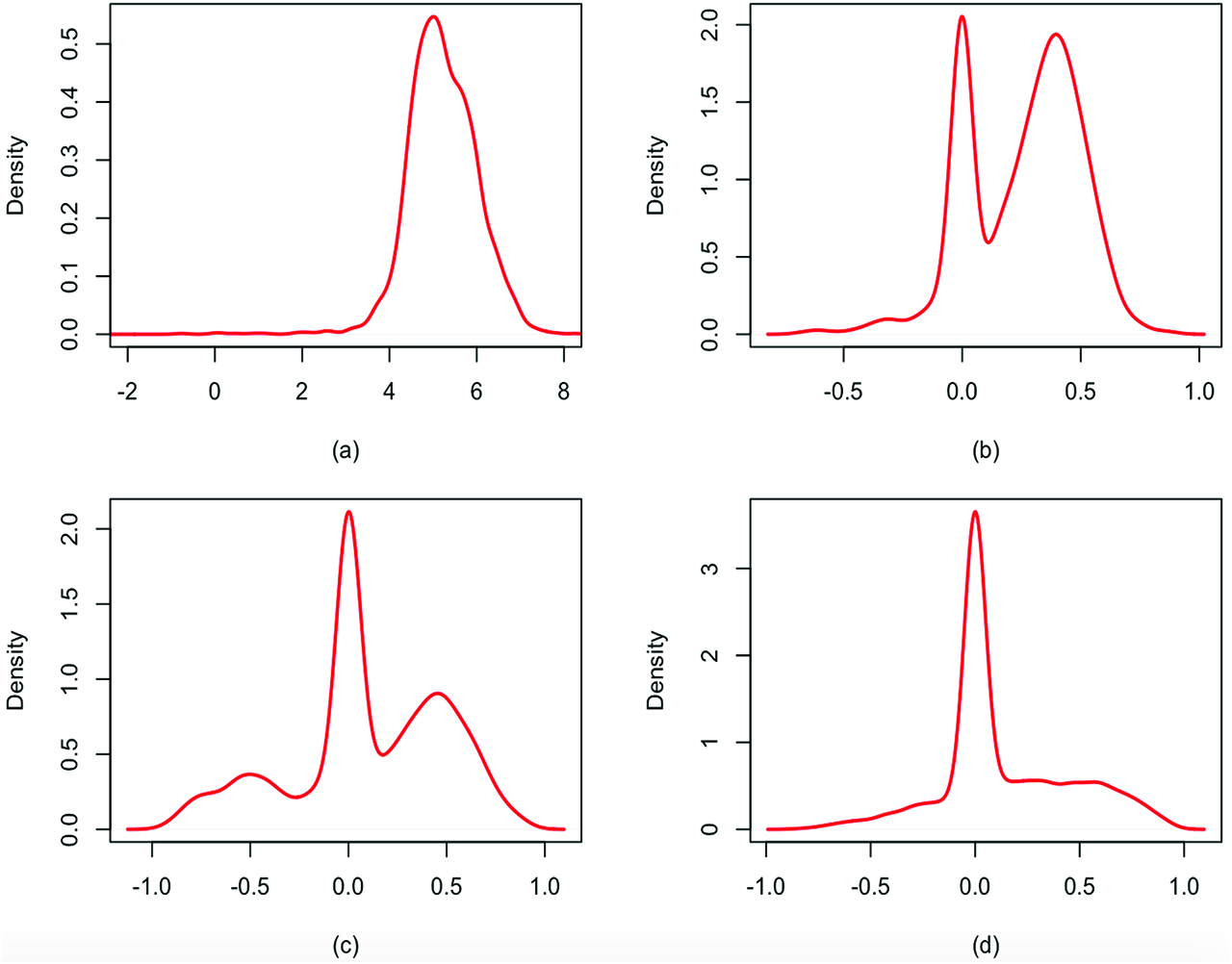
Readmission dataset: marginal posterior predictive distributions of mi0 (a), mi1 (b), mi2 (c) and mi3 (d) under the spike and slab prior.
5.2 Posterior analysis
We compare now the results of the nonparametric AR(2) model for the random effects αij’s as in (5)–(7), selected in the previous section, with models (2)–(3) built using different choices of g. In particular we consider two summary statistics:
In Figure 4 we present the marginal posterior predictive distributions of
Readmission dataset: posterior predictive distributions of
5.3 Posterior inference on the regression parameters
We now discuss the inference on the regression parameters in order to understand how covariates influence the recurrent event process. Although some covariates are fixed and do not vary over time, we still assume that their effect can be different in time and therefore we estimate a different vector of regression coefficients for all covariates in the model for each gap time j, j = 1, …,6. Covariates chemo and sex are binary variables, while dukes and charlson are 3 levels categorical variables and we need to introduce 2 dummy variables for each of them in the model, with baseline set to A–B for dukes and to 0 for charlson. Therefore, the final covariate vector for individual i is given by
Figure 5 displays 95 % credible intervals for the marginal posteriors of the regression parameter of each covariate for the first 5 gap times, i. e. of
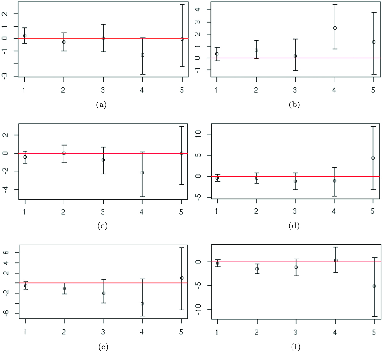
Readmission dataset: 95 % posterior credible intervals for the regression parameters of each covariate across the first five gap times. (a) Regression coefficients of chemo. (b) Regression coefficents of sex. (c) Regression coefficients of dukes = C. (d) Regression coefficients of dukes = D. (e) Regression coefficents of charlson = 1–2. (f) Regression coefficents of charlson = 3.
The dummy variable relative to Dukes stage C of the tumour and the regression coefficients corresponding to Dukes stage D are never significant. Finally, posterior CI’s of the parameters corresponding to the Charlson index show that, in general, patients with index 0 will have larger gap times with respect to the one with index 3, in fact the medians of the posterior distribution are concentrated on negative values. Moreover, credible intervals are larger for the last gap times, as expected, since few individuals have a large number of events. The regression coefficients at time j = 6 are not shown as the credible intervals are not comparable with those of the previous times.
5.4 Comparison with existing methods
In this subsection, we compare our model with the frequentist shared frailty model of [41] as implemented in the R package frailtypack [42]. In this setup the dependence between recurrences is modelled through a frailty variable, such that events which occur several times within the same subject during the period of observation share an unobserved random effect, i. e. frailty. The hazard function for the j-th event (
where h0(t) is the baseline hazard function,
Readmission dataset: estimates of the regression coefficients and associated p-values in the shared frailty model of [41].
| coef | p-value | |
|---|---|---|
| chemo | – 0.206 | 1.48e-01 |
| sex | – 0.537 | 1.06e-04 |
| dukes C | 0.297 | 6.42e-02 |
| dukes D | 1.056 | 5.82e-08 |
| charlson 1– 2 | 0.451 | 8.11e-02 |
| charlson 3 | 0.410 | 2.74e-03 |
The estimate of the variance θ of the frailty term is 0.67 with standard error 0.14, so θ is significantly different from 0, meaning that there is heterogeneity between subjects. Differently from our approach, in this model the regression coefficients do no vary across time. The most significant variables are the indicator for female, indicator for dukes equal to D and indicator for charlson equal to 3. A negative coefficient implies a lower risk of rehospitalization, while a positive a higher risk. In our analysis we obtain that (i) the coefficient for indicator of female (sex=1) remains in general positive over time, implying longer times between rehospitalizations; (ii) the coefficient for duke equal to D is initially negative but becomes positive for the last gap times; (iii) the regression parameters corresponding to charlson index equal to 3 are mostly negative over time. These results show a good agreement between the two models. Finally, Section 6 of Supplementary Material reports a comparison of our model with the dynamic frailty models of [26], who also adopt a Bayesian nonparametric approach based on the DP.
6 Urinary tract infection dataset
We consider data on patients at risk of urinary tract infection (UTI). The best clinical marker of UTI available is pyuria, i. e. White Blood Cell count (WBC) µl–1 (1/microliter) ≥ 1, detected by microscopy of a fresh unspun, unstained specimen of urine ([43, 44]). Let Ti0 correspond to the first visit attendance at the Lower Urinary Tract Service Clinic (Whittington Hospital, London, UK) and let Tij be the time of the j – th new infection for the patient i. Note that at time 0, all patients suffer of UTI. For each patient and at each visit the result of the microanalysis of a sample of urine has been recorded in terms of the WBC count. Presence of WBC in the urine (regardless of the quantity) indicates the presence of Urinary Tract Infection. We include in the analysis only female patients with at least two gap times, giving a total of N = 306 patients. The number of observations with exactly j gap times is displayed in Table 7.
UTI dataset: number of patients with exactly j gap times,
| j | 2 | 3 | 4 | 5 | 6 | 7 | 8 | 9 | TOT |
|---|---|---|---|---|---|---|---|---|---|
| nj | 121 | 89 | 54 | 21 | 10 | 6 | 2 | 3 | 306 |
We note that 85 subjects out of 306 are right-censored with respect to their last gap time. Since the proportion of censored data is considerable, we have taken censoring into account and modified the likelihood appropriately. Figure 6 displays the recurrent events of two randomly selected patients, in which the last gap time of the patient in the left panel is observed, while that of the patient in the right panel is censored. Indeed, the first patient suffers of infection at her last visit, while the second patient has a WBC count equal to zero implying that a new infection will happen necessarily after her last visit.
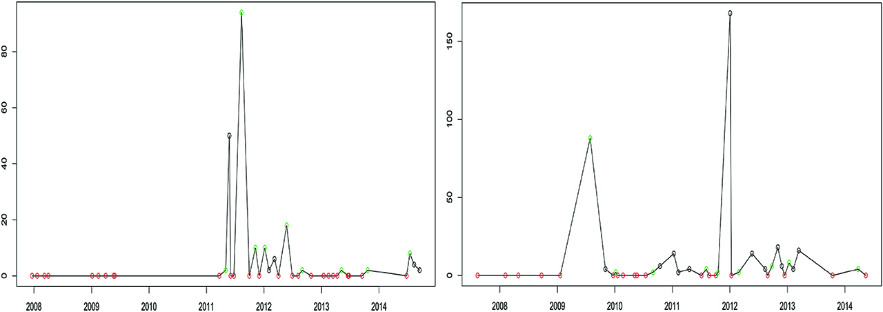
UTI dataset: recurrent events for two patients; the last gap time of the patient on the left is observed, while that of the patient on the right is censored. The vertical axis reports the value of WBC in the urine, red circles denote zero WBC at the visit while green circles denote WBC greater than 0.
We fit model (1), including for each patient a 5-dimensional vector of time-varying covariates: a continuous covariate representing the standardized age of the patient i during gap time j and four binary variables denoting the presence, during the j-th gap time, of urgency, pain, stress incontinence and voiding symptoms (=1 if the symptom is present, 0 otherwise). Therefore, the final covariate vector for individual i is given by
UTI dataset: descriptive statistics of the covariates.
| Covariate | Mean | Standard Deviation |
|---|---|---|
| age | 53.87 | 16.01 |
| presence of urgency symptoms | 0.56 | 0.50 |
| presence of incontinence symptoms | 0.21 | 0.41 |
| presence of pain symptoms | 0.47 | 0.50 |
| presence of voiding symptoms | 0.45 | 0.50 |
In the analysis we set the prior hyperparameters in (4) in order to specify vague prior distributions:
6.1 Posterior inference
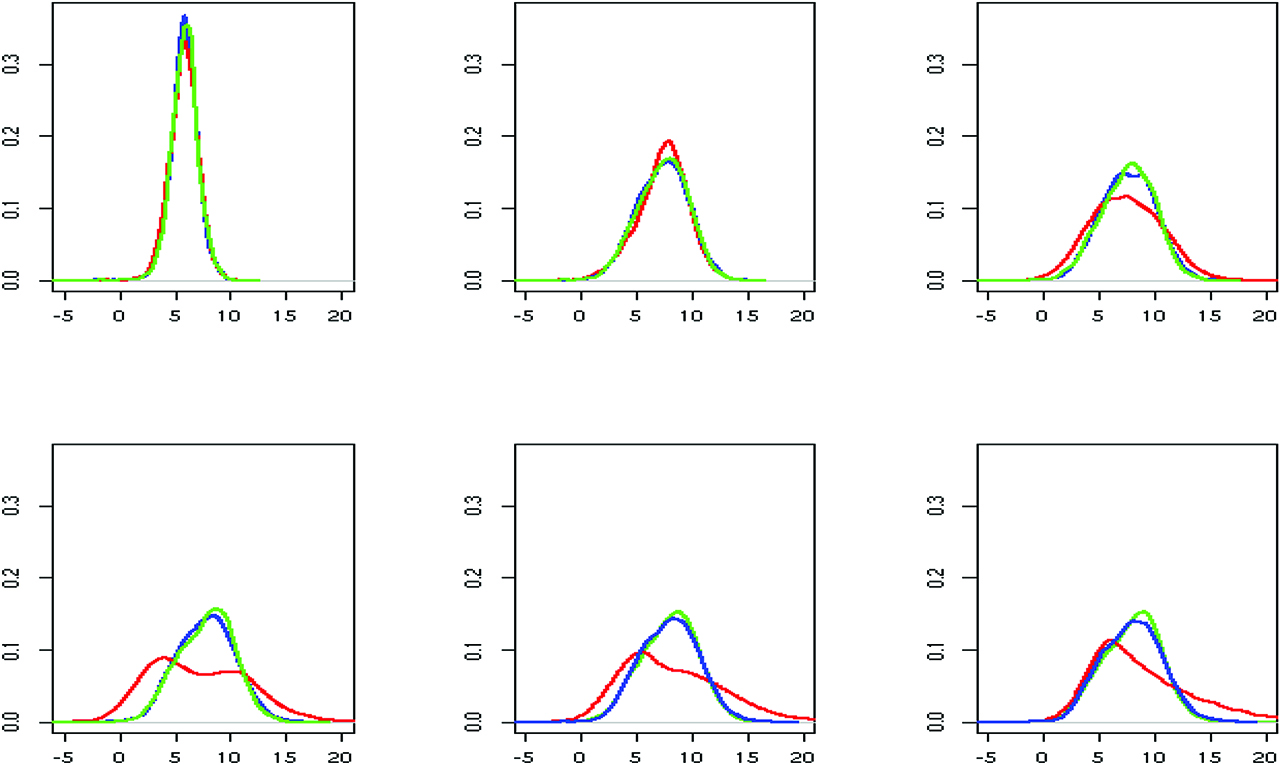
We perform inference on the order of dependence using both approaches introduced in Section 3. The marginal posterior predictive distributions of mi, l, for l = 0, 1, 2, 3, obtained with the spike and slab base measure, are displayed in red in Figure 7. Panels (b), (c) and (d) show that the predictive distributions of mi,1, mi,2, mi,3 are all concentrated around 0. In addition, specifying directly a prior on p, with P = 3, leads to a posterior distribution for the order of temporal dependence with mode in 0 (result shown in blue). These results indicate that there is no evidence of dependence between gap times, although the presence of a small cluster whose distribution is concentrated slight away from zero is detectable. This result is confirmed also by running the model for the three choices of function g described in Section 2.1, assuming an AR(1) structure. We obtain similar posterior predictive marginal distributions for mi0 and mi1, as well as the same posterior inference for K. In particular, a posteriori, the marginal distribution of mi1 is concentrated around 0, supporting the hypothesis of independence between gap times.
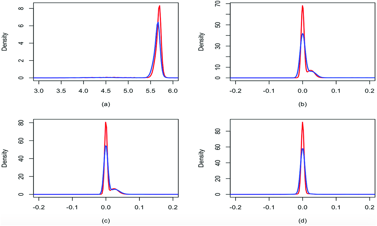
UTI dataset: marginal posterior predictive distributions of mi0 (a), mi1 (b), mi2 (c) and mi3 (d) obtained with the spike and slab base measure (red) and with the prior on the order of dependence (blue).
7 Conclusion
In this work we propose novel Bayesian nonparametric approaches for modelling gap times between recurrent events. Time-dependency is taken into account through the specification of an autoregressive model on the frailty parameters governing the distributions of the gap times. To allow for clustering of patients, overdispersion and outliers, we introduce Dirichlet process mixtures as random effects distribution. Both time-homogeneous and inhomogeneous covariates can be included in the model and we allow for their effect to vary through time.
The strategy we adopt is flexible and allows testing for the order of dependence among random effects at different times, that is a key feature of the nonparametric AR(p) model. We propose two different methods to test the order of dependence: spike and slab base measure and direct prior specification on the order of dependence. In the first case we can simply modify the base measure of the DP, whereas with the second technique, we elicit a prior on the order p of the autoregressive process and then, conditioning on p, we set a Dirichlet Process prior of appropriate dimension for the parameters of the AR(p) model.
We can introduce time-dependency between subject-specific gap times in different ways. The simplest and probably most natural way consists of assuming that the random effects at time j – 1, …, j – p influence the behaviour of the random effect at time j. We then investigate the possibility of approximating higher order of dependency using summary statistics of past observations. Our results show that the choice of summary statistics is crucial and not obvious and that the approximation worsens as the number of gap times increases. As such, this topic will be object of future research, possibly borrowing ideas from the Approximate Bayesian Computation literature.
In our model the random effect has a key clinical importance as it highlights the temporal evolution of the gap times. Our model allows for situations in which you can have independence among gap times as well as temporal dependence. This gives insight into the mechanisms of disease progression and the efficacy of medical interventions. In the cancer example, from Figure 3 it is evident that there is a time dependence between gap times, for some clusters of observations, up to order 2. For example, we find a cluster of individuals where there is a negative correlation with the second lag gap time. For another group this correlation is positive. These considerations have consequences on the expected length of time between events. On the other hand, there is no strong evidence of time dependency between gap times in the urinary infection example, which can impact therapeutic decisions.
The model strategy we propose can be extended to other fields of application; in particular it is straightforward to adapt the proposed approach to model multiple time series analysis [see [29, 45]. In fact, in this case, the data consist in N time series
Finally although the main focus of the paper is on modelling the recurrent event process itself, the proposed model can also be used as building block in a hierarchy to describe the relationship between recurrent events and survival up to a terminating event. In recent years there has been a surge of interest in methods for analysing recurrent events data with risk of termination dependent on the recurrent process [46]. This can be achieved by specifying a joint distribution of the gap times and event (termination) time. Let
where
with
References
[1] González JR, Fernandez E, Moreno V, Ribes J, Peris M, Navarro M, Cambray M, Borràs JM. Sex differences in hospital readmission among colorectal cancer patients. J Epidemiol Commun Health. 2005;59:506–11.10.1136/jech.2004.028902Search in Google Scholar PubMed PubMed Central
[2] Krege S, Giani G, Meyer R, Otto T, Rubben H. A randomized multicenter trial of adjuvant therapy in superficial bladder cancer: transurethral resection only versus transurethral resection plus mitomycin c versus transurethral resection plus bacillus calmette-guerin. J Urol. 1996;156:962–66.10.1097/00005392-199609000-00032Search in Google Scholar
[3] Ma Z, Krings AW. Multivariate survival analysis (i): shared frailty approaches to reliability and dependence modeling. In: 2008 IEEE Aerospace Conference, IEEE, 2008:1–21.10.1109/AERO.2008.4526618Search in Google Scholar
[4] Callens M, Croux C. Poverty dynamics in europe: a multilevel recurrent discrete-time hazard analysis. Int Sociol. 2009;24:368–96.10.1177/0268580909102913Search in Google Scholar
[5] Cook RJ, Lawless JF. The statistical analysis of recurrent events. New York: Springer, 2007.Search in Google Scholar
[6] Aalen O, Borgan O, Gjessing H. Survival and event history analysis: a process point of view. New York: Springer, 2008.10.1007/978-0-387-68560-1Search in Google Scholar
[7] Wang MC, Qin J, Chiang CT. Analyzing recurrent event data with informative censoring. J Am Stat Assoc. 2001;96:1057–65.10.1198/016214501753209031Search in Google Scholar PubMed PubMed Central
[8] Thall PF. Mixed poisson likelihood regression models for longitudinal interval count data. Biometrics. 1988;44:197–209.10.2307/2531907Search in Google Scholar
[9] Ma L, Sundaram R. Analysis of gap times based on panel count data with informative observation times and unknown start time. J Am Stat Assoc. 2016;113:294–305.10.1080/01621459.2016.1246369Search in Google Scholar
[10] Pepe MS, Cai J. Some graphical displays and marginal regression analyses for recurrent failure times and time dependent covariates. J Am Stat Assoc. 1993;88:811–20.10.1080/01621459.1993.10476346Search in Google Scholar
[11] Lawless JF, Nadeau C. Some simple robust methods for the analysis of recurrent events. Technometrics. 1995;37:158–68.10.1080/00401706.1995.10484300Search in Google Scholar
[12] Lawless J, Nadeau C, Cook R. Analysis of mean and rate functions for recurrent events. In: Proceedings of the First Seattle Symposium in Biostatistics, Springer, 1997:37–49.10.1007/978-1-4684-6316-3_4Search in Google Scholar
[13] Prentice RL, Williams BJ, Peterson AV. On the regression analysis of multivariate failure time data. Biometrika. 1981;68:373–9.10.1093/biomet/68.2.373Search in Google Scholar
[14] Chang SH, Wang MC. Conditional regression analysis for recurrence time data. J Am Stat Assoc. 1999;94:1221–30.10.1080/01621459.1999.10473875Search in Google Scholar
[15] McGilchrist C, Aisbett C. Regression with frailty in survival analysis. Biometrics. 1991;47:461–66.10.2307/2532138Search in Google Scholar
[16] Duchateau L, Janssen P. The frailty model. Springer Science & Business Media, 2007.Search in Google Scholar
[17] Lin LA, Luo S, Davis BR. Bayesian regression model for recurrent event data with event-varying covariate effects and event effect. J Appl Stat. 2018;45:1260–76.10.1080/02664763.2017.1367368Search in Google Scholar PubMed PubMed Central
[18] Chatterjee M, Sen Roy S. A copula-based approach for estimating the survival functions of two alternating recurrent events. J Stat Comput Simul. 2018;88:3098–115.10.1080/00949655.2018.1499741Search in Google Scholar
[19] Meyer R, Romeo JS. Bayesian semiparametric analysis of recurrent failure time data using copulas. Biometrical J. 2015;57:982–1001.10.1002/bimj.201400125Search in Google Scholar PubMed
[20] Antoniak CE. Mixtures of Dirichlet processes with applications to Bayesian nonparametric problems. Ann. Stat. 1974;2:1152–74.10.1214/aos/1176342871Search in Google Scholar
[21] Lo A. On a class of Bayesian nonparametric estimates: I. density estimates. Ann Stat. 1984;12:351–57.10.1214/aos/1176346412Search in Google Scholar
[22] Ferguson TS. A Bayesian analysis of some nonparametric problems. Ann Stat. 1973;1:209–30.10.1214/aos/1176342360Search in Google Scholar
[23] Sethuraman J. A constructive definition of Dirichlet priors. Stat Sin. 1994;4:639–50.10.21236/ADA238689Search in Google Scholar
[24] Müller P, Rosner GL. A Bayesian population model with hierarchical mixture priors applied to blood count data. J Am Stat Assoc. 92:1279–92.10.1080/01621459.1997.10473649Search in Google Scholar
[25] Kleinman KP, Ibrahim JG. A semiparametric Bayesian approach to the random effects model. Biometrics. 1998;54:921–38.10.2307/2533846Search in Google Scholar
[26] Pennell ML, Dunson DB. Bayesian semiparametric dynamic frailty models for multiple event time data. Biometrics. 2006;62:1044–52.10.1111/j.1541-0420.2006.00571.xSearch in Google Scholar PubMed
[27] Paulon G, De Iorio M, Guglielmi A, and Ieva F. Joint modeling of recurrent events and survival: a Bayesian non-parametric approach, 2018. https://dx.doi.org/10.1093/biostatistics/kxy026.Search in Google Scholar PubMed
[28] George E, McCullogh R. Variable selection via Gibbs sampling. J Am Stat Assoc 1993;88:881–89.10.1080/01621459.1993.10476353Search in Google Scholar
[29] Di Lucca MA, Guglielmi A, Müller P, Quintana FA. A simple class of Bayesian nonparametric autoregression models. Bayesian Anal. 2013;8:63–88.10.1214/13-BA803Search in Google Scholar PubMed PubMed Central
[30] Gelman A. Prior distributions for variance parameters in hierarchical models (comment on article by browne and draper). Bayesian Anal. 2006;1:515–34.10.1214/06-BA117ASearch in Google Scholar
[31] Clyde M, George EI. Model uncertainty. Stat Sci. 2004;19:81–94.10.1214/088342304000000035Search in Google Scholar
[32] George EI, McCulloch RE. Approaches for Bayesian variable selection. Stat Sin. 1997;7:339–73.Search in Google Scholar
[33] Kim S, Dahl DB, Vannucci M. Spiked Dirichlet process prior for Bayesian multiple hypothesis testing in random effects models. Bayesian Anal 2009;4:707–32.10.1214/09-BA426Search in Google Scholar PubMed PubMed Central
[34] Quintana FA, Müller P. Nonparametric Bayesian assessment of the order of dependence for binary sequences. J Comput Graphical Stat. 2012;13:213–31.10.1198/1061860042949Search in Google Scholar
[35] Carlin BP, Chib S. Bayesian model choice via markov chain monte carlo methods. J Royal Stat Soc Ser B (Methodological). 1995;57:473–84.10.1111/j.2517-6161.1995.tb02042.xSearch in Google Scholar
[36] Plummer M. JAGS: A program for analysis of Bayesian graphical models using Gibbs sampling, 2003.Search in Google Scholar
[37] Ishwaran H, Zarepour M. Exact and approximate sum representations for the Dirichlet process. Can J Stat. 2002;30:269–83.10.2307/3315951Search in Google Scholar
[38] Plummer M, Best N, Cowles K, Vines K. CODA: Convergence diagnosis and output analysis for MCMC. R News. 2006;6:7–11.Search in Google Scholar
[39] Kass RE, Carlin BP, Gelman A, Neal RM. Markov chain Monte Carlo in practice: a roundtable discussion. Am Stat. 1998;52:93–100.10.1080/00031305.1998.10480547Search in Google Scholar
[40] Manda SO, Meyer R. Bayesian inference for recurrent events data using time-dependent frailty. Stat Med. 2005;24:1263–74.10.1002/sim.1995Search in Google Scholar PubMed
[41] Rondeau V, Commenges D, Joly P. Maximum penalized likelihood estimation in a gamma-frailty model. Lifetime Data Anal. 2003;9:139–53.10.1023/A:1022978802021Search in Google Scholar
[42] Rondeau V, Mazroui Y, Gonzalez JR. frailtypack: an R package for the analysis of correlated survival data with frailty models using penalized likelihood estimation or parametrical estimation. J Stat Softw. 2012;47:1–28.10.18637/jss.v047.i04Search in Google Scholar
[43] Khasriya R, Khan S, Lunawat R, Bishara S, Bignal J, Malone-Lee M, Ishii H, O’Connor D, Kelsey M, Malone-Lee J. The inadequacy of urinary dipstick and microscopy as surrogate markers of urinary tract infection in urological outpatients with lower urinary tract symptoms without acute frequency and dysuria. J Urol. 2010;183:1843–7.10.1016/j.juro.2010.01.008Search in Google Scholar PubMed
[44] Kupelian AS, Horsley H, Khasriya R, Amussah RT, Badiani R, Courtney AM, Chandhyoke NS, Riaz U, Savlani K, Moledina M, Montes S, O’Connor D, Visavadia R, Kelsey M, Rohn JL, Malone-Lee J. Discrediting microscopic pyuria and leucocyte esterase as diagnostic surrogates for infection in patients with lower urinary tract symptoms: results from a clinical and laboratory evaluation. BJU Int. 2013;112:231–38.10.1111/j.1464-410X.2012.11694.xSearch in Google Scholar PubMed
[45] Nieto-Barajas LE, Quintana FA. A Bayesian non-parametric dynamic AR model for multiple time series analysis. J Time Ser Anal. 2016;37:675–89.10.1111/jtsa.12182Search in Google Scholar
[46] Sinha D, Maiti T, Ibrahim JG, Ouyang B. Current methods for recurrent events data with dependent termination: a bayesian perspective. J Am Stat Assoc. 2008;103:866–78.10.1198/016214508000000201Search in Google Scholar PubMed PubMed Central
Supplementary Material
The Supplementary Materials file includes further posterior inference under our models for the different simulated scenarios referenced in Section 4 (see Sections 1–2 there) and two extra simulation scenarios (Sections 3–4 there). Further posterior inference on the Readmission dataset is included in Section 5 and 6. Sections 7 and 8 contains the JAGS files.
The online version of this article offers supplementary material (DOI:https://doi.org/10.1515/ijb-2018-0088).
© 2020 Walter de Gruyter GmbH, Berlin/Boston
Articles in the same Issue
- Research Articles
- Efficient Nonparametric Causal Inference with Missing Exposure Information
- Simultaneous Inference of Treatment Effect Modification by Intermediate Response Endpoint Principal Strata with Application to Vaccine Trials
- Incorporating Contact Network Uncertainty in Individual Level Models of Infectious Disease using Approximate Bayesian Computation
- Bayesian Two-Stage Adaptive Design in Bioequivalence
- Exploration of Heterogeneous Treatment Effects via Concave Fusion
- Simple Quasi-Bayes Approach for Modeling Mean Medical Costs
- Bayesian Autoregressive Frailty Models for Inference in Recurrent Events
- Bayesian Detection of Piecewise Linear Trends in Replicated Time-Series with Application to Growth Data Modelling
- Cell Line Classification Using Electric Cell-Substrate Impedance Sensing (ECIS)
- On the Use of Optimal Transportation Theory to Recode Variables and Application to Database Merging