Bayesian Detection of Piecewise Linear Trends in Replicated Time-Series with Application to Growth Data Modelling
-
Panagiotis Papastamoulis

 ,
Takanori Furukawa
,
Takanori Furukawa

Abstract
We consider the situation where a temporal process is composed of contiguous segments with differing slopes and replicated noise-corrupted time series measurements are observed. The unknown mean of the data generating process is modelled as a piecewise linear function of time with an unknown number of change-points. We develop a Bayesian approach to infer the joint posterior distribution of the number and position of change-points as well as the unknown mean parameters. A-priori, the proposed model uses an overfitting number of mean parameters but, conditionally on a set of change-points, only a subset of them influences the likelihood. An exponentially decreasing prior distribution on the number of change-points gives rise to a posterior distribution concentrating on sparse representations of the underlying sequence. A Metropolis-Hastings Markov chain Monte Carlo (MCMC) sampler is constructed for approximating the posterior distribution. Our method is benchmarked using simulated data and is applied to uncover differences in the dynamics of fungal growth from imaging time course data collected from different strains. The source code is available on CRAN.
1 Introduction
In many applications a non-stationary time series consists of an unknown number of segments. The observed data is described by different statistical generative models within each segment. In such cases, the objective is to identify the number and position of change-points which give rise to different segments of the data as well as to infer all remaining parameters of the underlying statistical model. In principle, there are two approaches for answering these questions: online and offline segmentation [1], which refer to the task of inferring changes during or after the observation process, respectively. In this work, the latter scenario is considered.
We develop a Bayesian method for detecting an unknown number of change-points in the slope of multiple replicated time series. There are many methods for detecting change-points, with the majority of them focused on analysis of univariate time series (reviewed below). Our problem differs from these as we model changes in slope rather than fitting a step function to the mean, and we consider multiple time series with replication. For a given period t = 1, …, T we observe multiple time series which are assumed independent, each one consisting of multiple measurements (replicates). Each time series is assumed to have its own segmentation, which is common among its replicates. Thus, different time series have distinct mean structures in the underlying normal distribution.
Our method is motivated by the need to analyse fungal growth attributes on a massively parallel scale. Specifically, we are interested in identifying mutations which affect fitness in the major human fungal pathogen Aspergillus fumigatus. In such studies, growth is characterized by different phases which can be reasonably described by a piecewise linear model, as illustrated in Figure 1. Microbial growth is a complex characteristic which is heavily influenced by nutritional, metabolic, proliferative, physiological and genetic factors. Multiple techniques have been developed with which to quantify microbial growth, including direct quantitation of cell counts using flow cytometry or microscopy, colony counts, biomass quantitation, or indirect methods involving light scattering or turbidity measurement in liquid phase cultures, or dye-based methods. Optimisation of data acquisition and analysis has received rather less attention, particularly where the quantitation of growth characteristics in filamentous and aggregative microorganisms, such as A. fumigatus or Streptomyces coelicolor is complicated by the occurrence of one or several morphological shifts during the mitotic life cycle [2] leading to altered light scattering patterns dependent upon the size and shape of the particulate sample (bacteria or yeast), as well as difference in the index of refraction between the particles and the culture media [3]. In the latter instance an accurate means of defining the number and timing of change-points during growth curve analysis would significantly empower the optimisation of drug discovery screens where inhibitors of microbial growth might be sought; or in optimisation of biotechnological processes where moderation of microbial growth conditions to favour a particular growth phase might boost industrial production of enzymes or metabolites.
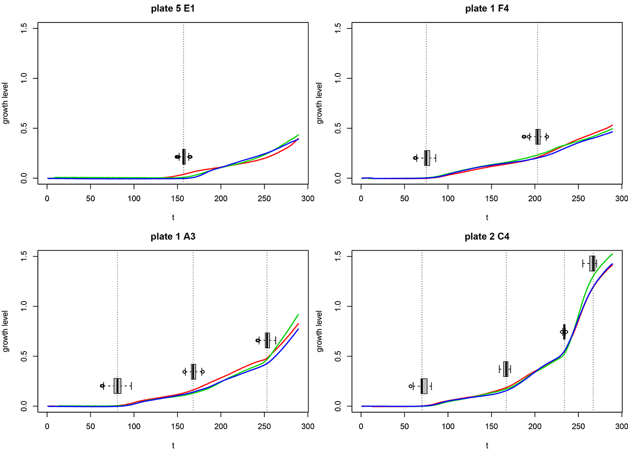
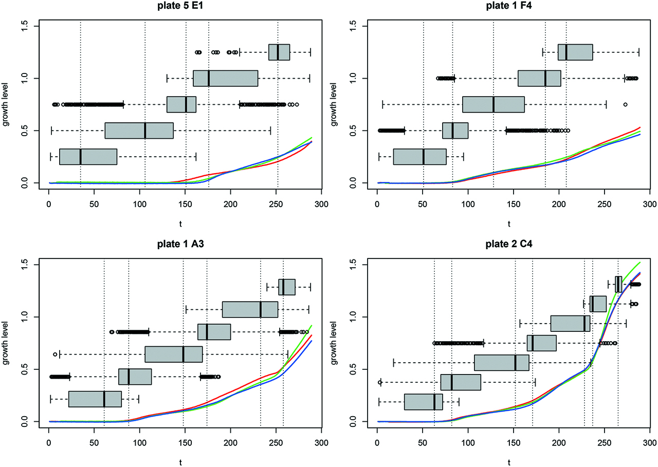
A subset of four growth data series described in Section 4.2, consisting of the growth level of three replicates (red, green and blue), measured every 10 minutes for a series of T = 289 time-points. The boxplots display the marginal posterior distribution of each change-point, conditionally on the inferred Maximum A Posteriori number of change-points according to the MCMC sampler detailed in Section 3.1.
In the seminal paper of Green [4], the Reversible Jump MCMC (RJMCMC) algorithm used to detect the number of change-points in coal mining disaster data. Subsequently, the RJMCMC methodology was applied to a variety of change-point detection problems [5, 6, 7, 8]. Lavielle and Lebarbier [9] proposed an MCMC sampler to estimate the number of change-points by introducing a latent sequence of independent and identically distributed Bernoulli random variables
Chib [11] formulates the change-point model in terms of a latent discrete state variable corresponding to the regime from which a particular observation has been drawn. The posterior distribution for a given number of change-points is then approximated using MCMC sampling, while inference on the number of change-points is carried out by estimating the marginal likelihood of the model using the method in Chib [12]. Fearnhead [13] discusses exact Bayesian inference by assuming that the joint posterior distribution of the parameters is independent across the segments of the time series and also presents an extension that allows the signal to perform a random walk within each segment. Other Bayesian methods include Dobigeon et al. [14], Hutter [16], Kim and Cheon [17], Rudoy et al. [18], Schütz and Holschneider [19], He [15], Schwaller and Robin [20]. In all of the aforementioned studies, change-points are defined via a step-function in the mean, assuming that segment parameters are independent. This is not the case in our approach, where we are explicitly imposing a continuity assumption between segments which allows us to detect changes in slope. With the exception of Dobigeon et al. [14], Schwaller and Robin [20], all other methods are focusing on univariate time-series.
There are relatively few studies looking specifically at a change-in-slope model [21] [22, 23, 24, 25], although they only consider a single time-series. Popular non-Bayesian methods such as binary segmentation [26, 27] do not work for detecting changes-in-slope [22]. Furthermore, standard dynamic programming approaches [28, 29] cannot be directly applied to our problem as discussed by Fearnhead et al. [24].
There is a wide range of non-Bayesian approaches to change-point estimation, see for example Halpern [32], Lu et al. [33], Picard et al. [34], Yildirim [35], Chamroukhi et al. [30], Frick et al. [31]. However, we choose a Bayesian approach for its competency in quantifying uncertainty and flexibility for incorporating prior information.
We construct a Metropolis-Hastings MCMC sampler [36, 37] for jointly inferring the number and position of change-points as well as the related mean parameters by adopting ideas from inference over sparse representations of sequences [10]. An advantage of our approach is that the proposed MCMC algorithm is straightforward to implement since it is based on standard Metropolis–Hastings move types and demands small modelling effort compared to other methods. Although exact integration is possible given the number and locations of change-points, it is time consuming hence we exploit the convenience of the MCMC sampler to approximately sample from the joint posterior distribution of the parameters. The dimensionality of the parameter space is fixed, thus our method avoids the complex step of designing trans–dimensional MCMC transitions as required by RJMCMC methods. Furthermore, we do not have to consider modified versions of the target posterior distribution [9], and there is no requirement for fitting the same model under different number of change-points and approximating the marginal likelihood for model selection.
The rest of the paper is organised as follows. Section 2 introduces the proposed model and the corresponding prior assumptions are presented in Section 2.1. The main MCMC sampler we use is detailed in Section 3.1. Sections 3.2 and 3.3 discuss variance estimation procedures, depending whether the variance is treated as a known parameter or not. The proposed method is illustrated in simulated and real data in Sections 4.1 and 4.2, respectively. The paper concludes in Section 5. More details on the simulation procedure and additional results are given in the Appendix.
2 Model
Let
independent (given the model parameters) for n = 1, …, N; t = 1, …, T; r = 1, …, R, where
For sample n and an unknown non-negative integer
Note that both the elements as well as the length of the ordered
where we also define
Thus, for sample n, conditionally on
independent for n = 1, …, N; t = 1, …, T; r = 1, …, R. Note that given
To be precise, the likelihood is defined as
where
2.1 Prior assumptions
For the mean parameters we assume that
independent for n = 1, …, N; t = 1, …, T. The quantities
In order to specify the prior distribution of locations for a given number of change-points (
Let
Note that according to eq. (8),
Finally, the prior distribution of the number of change-points should be defined. Recall that the distribution in eq. (1) assigns a distinct mean parameter per time-point. However, given
For a given number of change-points (
The prior
where
have exponential decrease (9) for
Finally, we mention that typical prior assumptions on the number of change-points (for example a truncated Poisson or a uniform distribution over a pre-specified set of non-negative integer values) tend to overfit the number of change-points. This behaviour is demonstrated in Section 4.1 using simulated data with a known number of change-points, as well as in Section C of the Appendix using our real dataset.
3 Inference
3.1 Metropolis–Hastings MCMC Sampler
Assume first that the variances
Although analytical evaluation of the marginal posterior distribution
At each step, the state of the chain is updated using four move-types: move 1 updates the number of change-points, move 2 updates the mean parameters by using a random walk proposal centered at the current values, move 3 updates the position of change-points and move 4 updates the subset of mean parameters that are not allocated to a change-point. In each case the proposed move is accepted according to the usual Metropolis-Hastings acceptance ratio, that is,
In eq. (13),
Move 1 This move updates the number of change-points, while keeping the mean parameters constant. We introduce two move types which propose to update the total number of change-points by 1. These move-types are complementary to each other: addition/deletion of a change-point. In the following,
At a given state consisting of
where L denotes the maximum number of change-points (
In the case of proposing deletion of a change-point
At this point we underline that using an overfitted set of model parameters (one mean
Move 2 In this move the update of mean parameters
independent for all t and n, for some constant c > 0. Recall that
Move 3.a The candidate state is generated by using a proposal distribution which will jointly update the change-points
where
independently for
where
Move 3.b This is a similar proposal to Move 3.b, but instead of proposing the simultaneous update of all cut-points, just one entry is modified and the rest remain the same. As in Move 3.a, both the number of change-points as well as the values of mean parameters remain the same. Thus, let
where
The Metropolis-Hastings acceptance probability simplifies to eq. (18). In this case, a sufficiently large value for
Move 4 Let
Note that both moves 3.a and 3.b are able to propose states that have zero prior probability in eq. (8). Although this is not a frequent event, in this case the proposed state is immediately rejected, since the prior probability ratio is equal to zero.
Recall that the previous MCMC steps are defined conditionally on
3.2 Variance estimation at a pre-processing stage
In this case the variance is considered known and in practice it should be estimated at a pre-processing stage. We use the posterior mean arising from a multivariate normal–inverse gamma model as a point estimate. For this purpose we ignore the piecewise linear parameterization of the mean function and use the same likelihood as in eq. (1) and the same prior assumptions for
We will assume two parameterizations: the full model where the variances are a-priori distributed as:
independent for n = 1, …, N; t = 1, …, T, where
Under (21), a-priori it is assumed that
independent for t = 1, …, T. The quantities
Let us define the function
for t = 1, …, T; n = 1, …, N. It easily follows that under (20):
independent for n = 1, …, N; t = 1, …, N. In the case of the restricted parameterization in (21), the corresponding posterior distribution is
independent for t = 1, …, T. Then, we use the posterior means as the plug-in point estimates of the variance per time-point, that is,
provided that
3.3 Updating the variance
Here we discuss the case where the variance in eq. (1) is unknown. In the case where all variances are unrestricted (eq. (20)), the full conditional distributions are:
independent for n = 1, …, N, t = 1, …, T. Note that in this case, the full conditional distribution depends on the piecewise linear mean function
independent for t = 1, …, T.
We will use the labels “s3” and “s4” to refer to the MCMC sampler using the Gibbs steps (20) and (21), respectively. Since the full conditional distribution of
4 Results
4.1 Simulation study
We considered simulated datasets of length T = 1000 time-points consisting of N = 1000 independent multivariate observations, while the number of replicates (R) is equal to R = 3. For n = 1, …, N, the number of change-points
All three samplers were applied using the following set of hyper-parameter values:
Our results are benchmarked against the not package available in the Comprehensive R Archive Network, which implements the narrowest-over-threshold method of Baranowski et al. [22]. The number of change-points is inferred using a strengthened version of the Bayesian Information Criterion [26, 38]. For the problem of detecting changes in the slope, this approach only considers univariate time-series with constant variance, thus, it is not suitable for multivariate time-series where the variance varies with time (which is the case in our datasets). In order to apply this method we averaged across the replicates of the time-series.
Figure 2 displays the difference of the estimated number of change-points (
![Figure 2: Benchmarking the estimation of the number of change-points arising from the narrowest-over-threshold (“not”) method of [22] and our MCMC sampler with fixed different variance (s1), fixed shared variance (s2) and unknown different variance (s3) per time-series, under the complexity prior distribution. The number after the name of each sampler indicates the true number of change-points and for each value 100 synthetic datasets were simulated. Each time-series consists of three replicates and 1000 time-points.](/document/doi/10.1515/ijb-2018-0052/asset/graphic/j_ijb-2018-0052_fig_002.jpg)
Benchmarking the estimation of the number of change-points arising from the narrowest-over-threshold (“not”) method of [22] and our MCMC sampler with fixed different variance (s1), fixed shared variance (s2) and unknown different variance (s3) per time-series, under the complexity prior distribution. The number after the name of each sampler indicates the true number of change-points and for each value 100 synthetic datasets were simulated. Each time-series consists of three replicates and 1000 time-points.
We conclude that in many cases the method of [22] tends to overfit the number of change-points, resulting to worse performance than our method. Clearly, benchmarking against this simpler approach should not be perceived as a fair comparison between the two methods, but as a means of highlighting the usefulness of our modelling.
Figure 3 displays the output of the MCMC sampler s1 (lower panel) and s2 (upper panel) for a time-series where the true number of change-points equals to 8. The output of sampler s3 is almost identical to the lower panel of Figure 3. The posterior distribution of the number of change-points is shown at the left panels, considering both the complexity prior distribution (gray trace) as well as a Poisson(1) distribution truncated on the set {0, 1, …, 30}. Observe that the first choice quickly converges to a state with 8 change-points (that is, the true number). This is not the case under the Poisson prior distribution, which supports larger values than the true number of change-points. This behaviour is typical in other simulated datasets we tried, therefore, all results in the remaining sections are based on the complexity prior. The right panels display the posterior distribution of change-point locations (under the complexity prior) and it evident that the method is able to accurately infer all change-point locations.
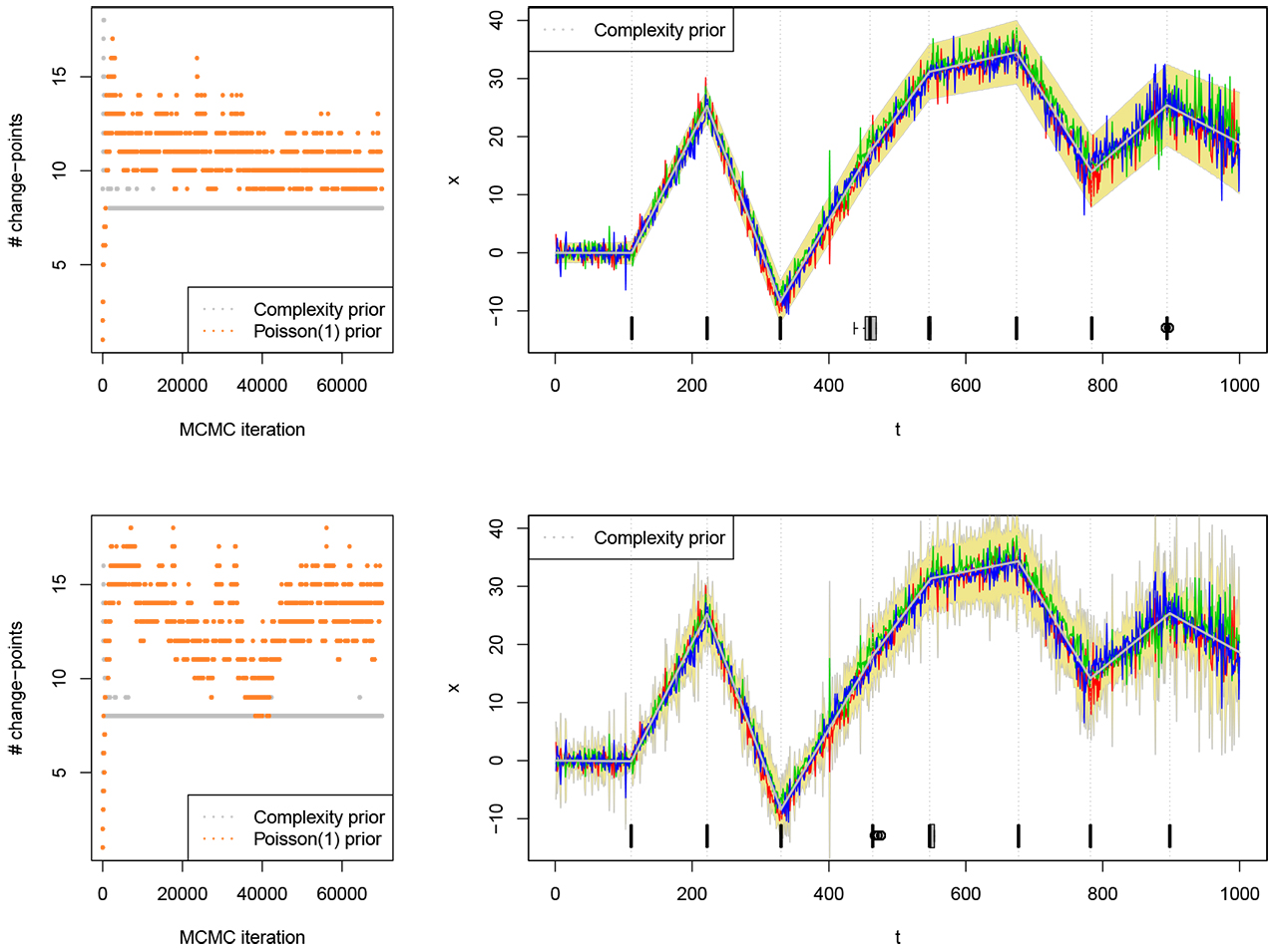
Example of a simulated time-series with 8 change-points. Replicates are shown in red, blue and green color. Left: MCMC trace of the sampled number of change-points considering both the complexity and a truncated Poisson(1) prior distributions (every 20th iteration is displayed). Right: output of the MCMC sampler conditionally on the estimated MAP of changepoints (which is equal to 8) according to the complexity prior. The upper and lower panels correspond to the MCMC sampler using the variance estimates arising from eq. (23) (sampler s2) and (22) (sampler s1), respectively. The gray lines correspond to the posterior mean estimates of the piecewise linear mean function and the boxplots display the posterior marginal distribution of each change-point. Vertical dotted lines correspond to the central line of each boxplot (median). The coloured outer regions correspond to two estimated standard deviations from the mean.
Additional results based on synthetic data are provided in Section B of the Appendix, including prior sensitivity checks as well as alternative simulation scenarios. Further comparisons against not are provided in Section D of the Appendix.
4.2 Phase detection in parallel time-series analysis of fungal growth
The filamentous fungal pathogen Aspergillus fumigatus is a major pathogen of the human lung causing more deaths per annum than tuberculosis or malaria [39]. A time series study of fungal growth was performed in liquid culture by analysing, in parallel, the growth characteristics of 411 independent transcription factor gene deletion mutants. The mutant strains were cultivated in a microtiter plate containing 200 µL of a fungal culture medium and incubated at 37 °C. Optical density (at 600 nm) was measured at 10 minute intervals for a total period of 48 hours. The growth analysis was performed on three separate occasions.
The observed data consists of N × R × T growth levels for R = 3 replicates of N = 411 objects (mutants) measured every 10 minutes for T = 289 time-points. Figure 1 displays the observed time series for four mutants. Visual inspection reveals that describing growth with a piecewise linear mean function with an unknown number of segments is a reasonable assumption for the observed data. Regarding the fixed hyper-parameter values, we considered that α = 2 (eq. (10)) and
The boxplots in Figure 1 correspond to the estimate of the marginal posterior distribution of each change-point for specific subset of four mutants, conditionally on the mode of the posterior distribution of the number of change-points. Figure 4 displays the averaged profile per mutant (mean of three replicates) coloured according to the most probable number of change-points for each of N = 411 subjects. We conclude that the majority of the mutants (343) consist of three growth phases. It is clear that mutants with a smaller number of change-points are also the more slowly growing mutants, which is reasonable since these mutants most likely have not been able to reach the later growth phases in the time of the experiment. In particular the method inferred 35 mutants with only 2 growth phases and slow growth behaviour while 12 mutants have a single phase and very slow growth behaviour. Finally, 21 mutants consist of 4 growth phases and some of them exhibit a faster growth rate at later observation stages (t > 220).
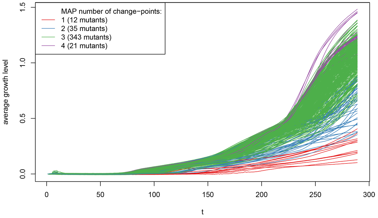
Visualization of the growth dataset with respect to the estimated MAP number of phases. For plotting convenience, each curve corresponds to the average growth time series across the three replicates.
Amongst 12 fungal mutants identified as having a single change-point during growth curve analysis, and therefore exhibiting severely retarded growth kinetics, seven mutants had previously been characterised [40, 41, 42, 43, 44, 45]. Without exception previously characterised mutants had been reported as having various morphological defects, and these morphogenesis mutants were correctly identified in our analysis. The remaining five mutants have, until now, remained uncharacterised and therefore provide promising candidates to investigate further in order to establish their roles in fungal morphogenesis. Detailed phenotypical characterisations of the identified mutants will be described elsewhere.
a
We have also considered a Poisson(1) prior distribution on the number of change-points. As already demonstrated in Section 4.1, in this case the sampler selects a larger number of change-points which are less interpretable. The reader is referred to Section C of the Appendix.
5 Discussion
A method for inferring the number of change-points in the underlying piecewise linear mean function of replicated time-series has been presented. A crucial characteristic of the model is that each time-point may have its own mean, an assumption which introduces an overfitting number of parameters. The method is able to penalize overfitting models by using an exponentially decreasing prior distribution [10] on the number of change-points and it was demon strated that this approach leads to a posterior distribution that can accurately recover the underlying sparse structure of the model.
We considered that the variance may be fixed or treated as unknown. In the first case we used a plug-in estimate arising from a pre-processing stage of the data. Moreover two different variance parameterizations were introduced, depending on whether the variance of each time-point is shared between different time-series or not. We have also discussed the case where the variance is treated as unknown, updating its state by an extra Gibbs sampling step. According to our simulations, the samplers with fixed variance (s1 and s2) are quite competitive with the sampler s3 which also updates the variance.
There are many interesting extensions of our research. For example, one could assume more general models between replicates, such as a multivariate normal distribution with full covariance matrix and/or replicate-dependent means, or even models that are not necessarily normal. The core mechanism of the proposed MCMC sampler will be the same in these situations and it would be interesting to investigate whether the method can produce robust results in such settings. In our setup we observed that our sampler does not face any convergence issues and quickly reaches to a state where the number of change-points reflects the underlying structure of the model. In the previously mentioned generalizations however, it might be beneficial to seek ways of improving the mixing and accelerating convergence by e.g. embedding our sampler to parallel-tempering schemes. Another interesting extension of our research is to explore the usage of data transformations for stabilizing the variance of time series along time.
In our biological application, we found that all of the slow-growing mutant strains identified by our method, and which had previously been characterised in the literature, were known to play roles in fungal morphogenesis. Further experiments are planned to explore how the growth dynamics of the mutants considered here changes under different environmental conditions. Our simple change-point method provides a useful low-dimensional model of the growth dynamics to explore gene-environment effects on the growth phenotype.
6 Software and data availability
Our algorithm is available as an R package [46] at the Comprehensive R Archive Network [47]. Scripts to reproduce real and simulated data analysis are available online at https://github.com/mqbssppe/growthPhaseMCMC.
Funding source: Medical Research Council
Award Identifier / Grant number: MR/M02010X/1
Funding statement: Research was funded by MRC award MR/M02010X/1(Funder Id: http://dx.doi.org/10.13039/501100000265).
Acknowledgements
The authors would like to acknowledge the assistance given by IT services and use of the Computational Shared Facility of the University of Manchester. The suggestions of two anonymous reviewers helped to improve the findings of this study.
Conflicts of interest: The authors have declared no conflict of interest.
A Details of the MCMC sampler
The following pseudo-code summarizes the workflow of the proposed Metropolis–Hastings MCMC sampler for samplers s1 and s2.
For n = 1, …, N
Give some initial values
For m = 1, …, M
Move 2: Propose to update the mean parameters and accept the candidate state
Propose to update the change-points: with probability 0.5 choose Move 3.a, otherwise choose Move 3.b. Accept the candidate state
Move 4: Update the mean parameters that are not allocated to a change-point by sampling from the prior distribution.
In the case that the variance is unknown,the sampler is augmented by an extra Gibbs sampling step, which will update the variances using the full conditional distributions descibed in Section 3.3 of the paper.
In the presented applications we considered that the total number of MCMC iterations is equal to M = 70000, while the first 20000 are discarded as burn-in period. The parameters of the MCMC sampler are defines as follows: c = 0.05 (Move 2),
B Simulation study details
We considered simulated datasets of length T = 1000 time-points consisting of N = 1000 independent multivariate observations. Three simulated datasets of dimensionality N × R × T were genera ted according to (4) considering that the number of replicates (R) is equal to R = 3 or 6. For n = 1, …, N, the number of change-points
where
Recall that our model assumes that the replicates are iid random variables for a given time-point t and time-series n. However, we would rather benchmark our method in case that this assumption is not necessarily true. In order to introduce extra noise between replicates we assumed that the true change-point for each replicate has some variation around the time-point in eq. (26). Therefore, it was considered that replicate r changes its mean function at time
where
Each replicate was allowed to have some variation around the endpoints of each phase according to the
B.1 Simulation study 1: different variance per time-series
Regarding the observation variance
independent for t = 1, …, T and n = 1, …, N. Note that
Figure 5 illustrates a random subset of 10 simulated time-series with a number of change-points ranging in 0, 1, …, 9. Note that there is strong heterogeneity between time-series and that there are instances where replicates deviate from the iid assumption. We will refer to the specific data generation procedure with the term “noisy scenario”. Note that when d = 0 in eq. (27) and
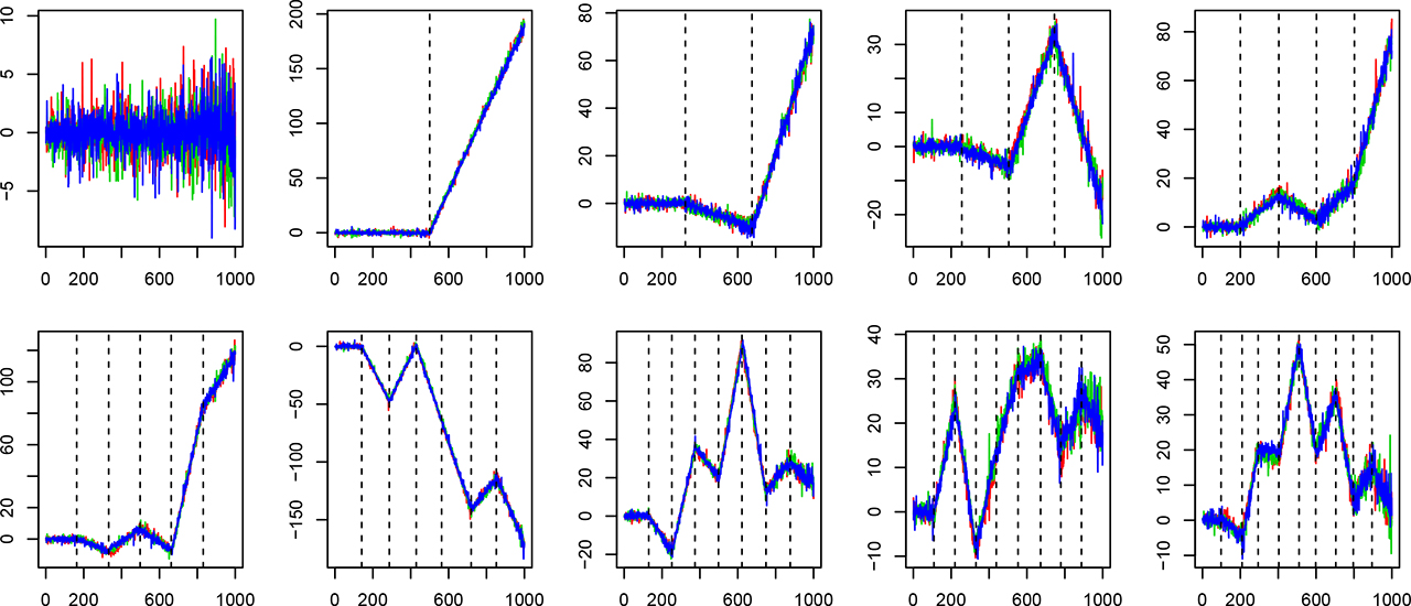
An example of 10 subjects from the simulated time-series with T = 1000 time-points with 3 replicates (blue, red, green) and number of change-points equal to 0, 1, …, 9 (indicated by dashed vertical lines).
Next we perform some prior sensitivity checks by considering different combinations of the hyper-parameters. Figure 6 shows the selected number of change-points using the approximate MAP estimate from the MCMC sample. Prior-sensitivity checks are performed by considering that α ∈ {1, 2} in eq. (10),
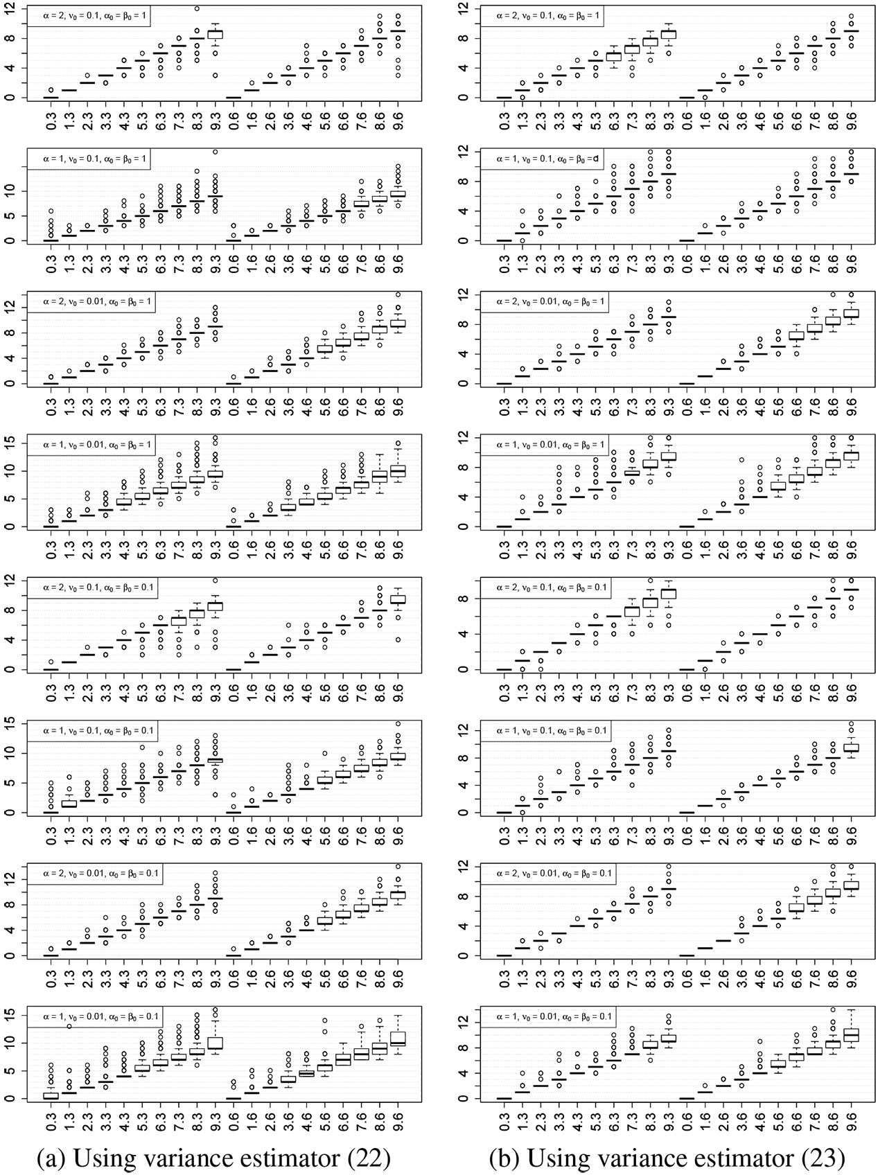
Estimation of the number of change-points on synthetic datasets generated under different variance per time series. The variance was estimated according to (a): the different variance estimator (22) and (b): the same variance estimator (23). Different combinations of prior parameters
B.2 Simulation study 2: same variance per time-series
In this section we replicate the “noisy” simulation scenario of Section B but now the variance is restricted to be the same between time series. More specifically, it is assumed that
independent for t = 1, …, T. Furthermore, we also consider the “exact” simulation scenario where no additional noise is introduced between replicates and expression levels. In order to estimate the variance per time point and time series we used the estimator in (23). Then, the MCMC sampler was run with the same number of iterations and burn-in period as previously (70000 and 20000, respectively).
The estimate of the number of change-points are shown in Figure 7(a) and Figure 7(b) for the noisy and exact simulation scenarios. We should note that the results are improved when replicating the analysis based on simulated datasets which are generated exactly by the assumed model, as illustrated in Figure 7(b), particularly when α = 1 and
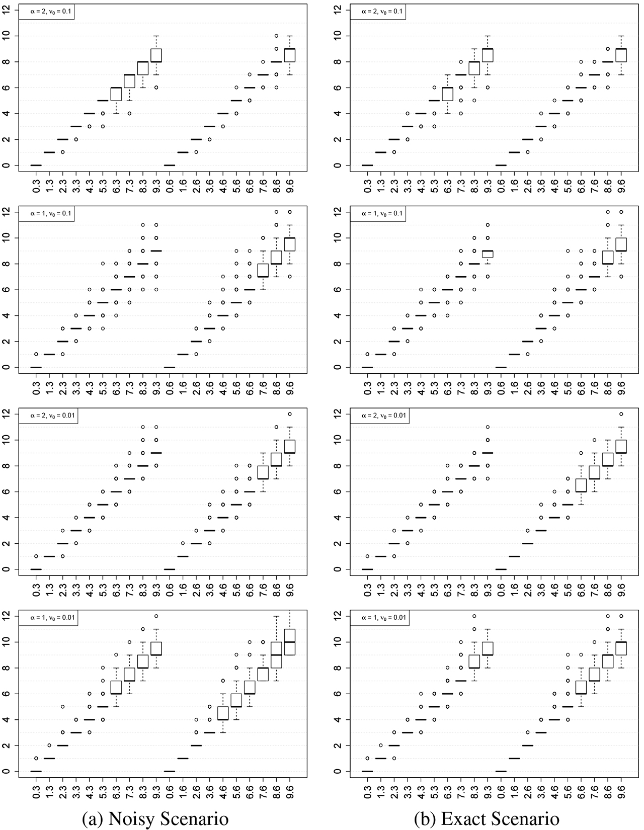
Benchmarking the estimation of the number of change-points on synthetic datasets according to the “noisy” and “exact” simulation scenarios. Different combinations of prior parameters
C Benchmarking against the Poisson distribution on the real dataset
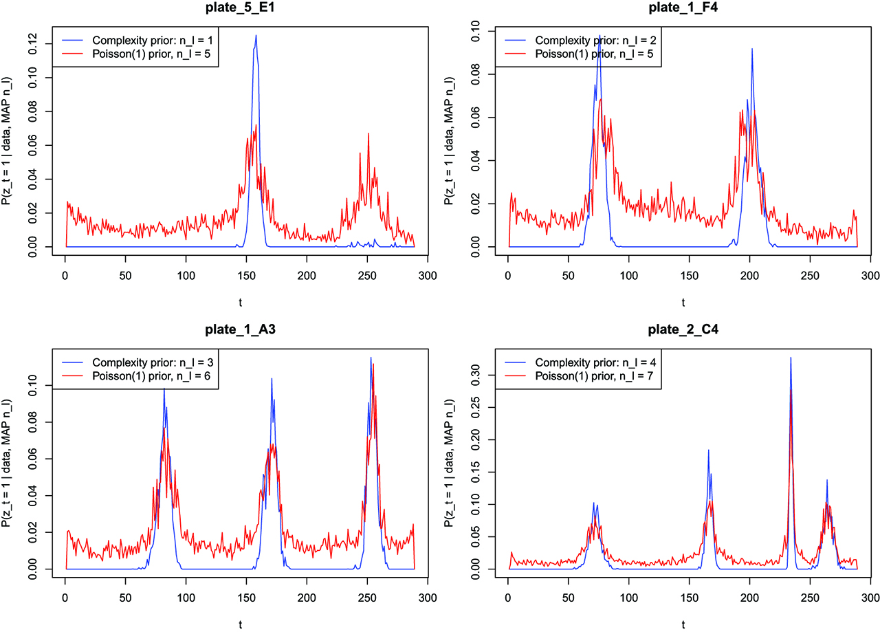
Recall that in Section 4.1 we demonstrated, using simulated data, that the estimated number of change-points tends to overfit when using a Poisson instead the complexity prior distribution. Here, we illustrate that this is also the case on our real dataset. We consider again a Poisson(1) distribution, truncated on the set {0, 1, …, 30} and use the same four time-series of the real dataset, depicted in Figure 1 of the main paper. As shown in Figure 8, the posterior distribution of the number of change-points under the Poisson prior distribution supports much larger values than the complexity prior. The estimated posterior mode of the number of change-points correspond to 5 for “plate 5 E1” (instead of 1 under the complexity prior), 5 for “plate 1 F4” (instead of 2), 6 for “plate 1 A3” (instead of 3) and 7 for “plate 2 C4” (instead of 4). We conclude that in this case the sampler assigns additional change-points to intermediate observation periods, compared to the ones selected under the complexity prior. These additional change-points identify very small changes in the slope of the time-series and they do not contribute much in the interpretation of growth characteristics.
Change-point locations conditionally on the MAP number of change-points according to a Poisson(1) prior distribution, truncated on the set {0, 1, …, 30} for four time-series of our real dataset.
In order to further inspect the differences between the results arising from the two different prior assumptions, let us define the following random variables:
for t = 1, …, T, n = 1, …, N. Note that
Estimated posterior probabilities of the binary state variables
D Additional benchmarking against the narrowest-over-threshold method
In this section we provide some additional results regarding synthetic and true datasets when using the not package of Baranowski et al. [22]. We consider one of our simulated datasets as well as one time-series of our real data, which illustrate the typical performance of each method in our data. As already mentioned, not deals with univariate time-series so in order to apply this method we averaged across the replicates of the time-series. The results are illustrated in Figure 10. The first column consists of a simulated dataset (using the same generating mechanism described in Section B, where the number of change-points is equal to 3 and our proposed method is able to succesfully detect it (shown in first row of Figure 10). On the other hand, the method of Baranowski et al. [22] overfits the number of change-points. A similar pattern is illustrated for the real dataset shown in the second column of Figure 10, where the narrowest-over-threshold method infers a much larger number of change-points compared to our approach, which is not realistic.
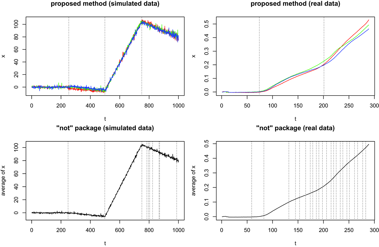
Comparison with the narrowest-over-threshold method as implemented in the not R package. Inferred change-points are indicated by dotted lines.
References
[1] Basseville M, Nikiforov IV. Detection of abrupt changes: theory and application Vol. 104. Englewood Cliffs: Prentice Hall, 1993Search in Google Scholar
[2] Fischer M, Sawers RG. A universally applicable and rapid method for measuring the growth of Streptomyces and other filamentous microorganisms by methylene blue adsorption-desorption. Appl Environ Microbiol. 2013;79:4499–502.10.1128/AEM.00778-13Search in Google Scholar
[3] Stevenson K, McVey AF, Clark IB, Swain PS, Pilizota T. General calibration of microbial growth in microplate readers. Sci Rep. 2016;6:38828.10.1038/srep38828Search in Google Scholar
[4] Green PJ. Reversible jump Markov chain Monte Carlo computation and Bayesian model determination. Biometrika. 1995;82:711–32.10.1093/biomet/82.4.711Search in Google Scholar
[5] Johnson TD, Elashoff RM, Harkema SJ. A Bayesian change-point analysis of electromyographic data: detecting muscle activation patterns and associated applications. Biostatistics. 2003;4:143. DOI: 10.1093/biostatistics/4.1.143.Search in Google Scholar
[6] Punskaya E, Andrieu C, Doucet A, Fitzgerald WJ. Bayesian curve fitting using MCMC with applications to signal segmentation. IEEE Trans Signal Process. 2002;50:747–58.10.1109/78.984776Search in Google Scholar
[7] Tai YC, Kvale MN, Witte JS. Segmentation and estimation for SNP microarrays: A Bayesian multiple change-point approach. Biometrics. 2010;66:675–83. DOI: 10.1111/j.1541-0420.2009.01328.x.Search in Google Scholar
[8] Zhao X, Chu P-S. Bayesian changepoint analysis for extreme events (typhoons, heavy rainfall, and heat waves): An RJMCMC approach. J Clim. 2010;23:1034–46.10.1175/2009JCLI2597.1Search in Google Scholar
[9] Lavielle M, Lebarbier E. An application of MCMC methods for the multiple change-points problem. Signal Process. 2001;81:39–53.10.1016/S0165-1684(00)00189-4Search in Google Scholar
[10] Castillo I, van der Vaart A. Needles and straw in a haystack: Posterior concentration for possibly sparse sequences. Ann Stat. 2012;40:2069–101. DOI: 10.1214/12-AOS1029.Search in Google Scholar
[11] Chib S. Estimation and comparison of multiple change-point models. J Econometrics. 1998;86:221–41. http://www.sciencedirect.com/science/article/pii/S0304407697001152.10.1016/S0304-4076(97)00115-2Search in Google Scholar
[12] Chib S. Marginal likelihood from the Gibbs output. J Am Stat Assoc. 1995;90:1313–21.10.1080/01621459.1995.10476635Search in Google Scholar
[13] Fearnhead P. Exact and efficient Bayesian inference for multiple changepoint problems. Stat Comput. 2006;16:203–13.10.1007/s11222-006-8450-8Search in Google Scholar
[14] Dobigeon N, Tourneret J-Y, Scargle JD. Joint segmentation of multivariate astronomical time series: Bayesian sampling with a hierarchical model. IEEE Trans Signal Process. 2007;55:414–23.10.1109/TSP.2006.885768Search in Google Scholar
[15] He C. Bayesian multiple change-point estimation for exponential distribution with truncated and censored data. Commun Stat - Theo Methods. 2017;46:5827–39. DOI: 10.1080/03610926.2016.1161797.Search in Google Scholar
[16] Hutter M. Exact Bayesian regression of piecewise constant functions. Bayesian Anal. 2007;2:635–64. DOI: 10.1214/07-BA225.Search in Google Scholar
[17] Kim J, Cheon S. Bayesian multiple change-point estimation with annealing stochastic approximation Monte Carlo. Comput Stat. 2010;25:215–39. DOI: 10.1007/s00180-009-0172-x.Search in Google Scholar
[18] Rudoy D, Yuen SG, Howe RD, Wolfe PJ. Bayesian change-point analysis for atomic force microscopy and soft material indentation. J R Stat Soc: Ser C (Appl Stat). 2010;59:573–93. DOI: 10.1111/j.1467-9876.2010.00715.x.Search in Google Scholar
[19] Schütz N, Holschneider M. Detection of trend changes in time series using Bayesian inference. Phys. Rev. E. 2011;84:021120. DOI: 10.1103/PhysRevE.84.021120.Search in Google Scholar PubMed
[20] Schwaller L, Robin S. Exact bayesian inference for off-line change-point detection in tree-structured graphical models. Stat Comput. 2017;27:1331–45. DOI: 10.1007/s11222-016-9689-3.Search in Google Scholar
[21] Stephens DA. Bayesian Retrospective Multiple-Changepoint Identification. Applied Statistics. 1994;43:159–159. DOI: 10.2307/2986119.Search in Google Scholar
[22] Baranowski R, Chen Y, Fryzlewicz P. Narrowest-over-threshold detection of multiple change-points and change-point-like features, 2016. arXiv preprint arXiv:1609.00293.Search in Google Scholar
[23] Cahill N, Rahmstorf S, Parnell AC. Change points of global temperature. Environ Res Lett. 2015;10:084002. http://stacks.iop.org/1748-9326/10/i=8/a=084002.10.1088/1748-9326/10/8/084002Search in Google Scholar
[24] Fearnhead P, Maidstone R, Letchford A. Detecting changes in slope with an l0 penalty. J Comput Graphical Stat. 2018;0:1–11. DOI: 10.1080/10618600.2018.1512868.Search in Google Scholar
[25] Schroeder AL, Fryzlewicz P. Adaptive trend estimation in financial time series via multiscale change-point-induced basis recovery. Stat Its interface. 2013;6:449–61.10.4310/SII.2013.v6.n4.a4Search in Google Scholar
[26] Fryzlewicz P. Wild binary segmentation for multiple change-point detection. Ann Stat. 2014;42:2243–81. DOI: 10.1214/14-AOS1245Search in Google Scholar
[27] Scott AJ, Knott M. A cluster analysis method for grouping means in the analysis of variance. Biometrics. 1974;30:507–12. http://www.jstor.org/stable/2529204.10.2307/2529204Search in Google Scholar
[28] Jackson B, Scargle JD, Barnes D, Arabhi S, Alt A, Gioumousis P, et al. An algorithm for optimal partitioning of data on an interval. IEEE Signal Process Lett. 2005;12:105–8.10.1109/LSP.2001.838216Search in Google Scholar
[29] Killick R, Fearnhead P, Eckley IA. Optimal detection of changepoints with a linear computational cost. J Am Stat Assoc. 2012;107:1590–8.10.1080/01621459.2012.737745Search in Google Scholar
[30] Chamroukhi F, Mohammed S, Trabelsi D, Oukhellou L, Amirat Y. Joint segmentation of multivariate time series with hidden process regression for human activity recognition. Neurocomputing. 2013;120:633–644. http://www.sciencedirect.com/science/article/pii/S0925231213004086, image Feature Detection and Description.10.1016/j.neucom.2013.04.003Search in Google Scholar
[31] Frick K, Munk A, Sieling H. Multiscale change point inference. J R Stat Soc: Ser B (Stat Method). 2014;76:495–580. DOI: 10.1111/rssb.12047.Search in Google Scholar
[32] Halpern AL. Multiple-changepoint testing for an alternating segments model of a binary sequence. Biometrics. 2000;56:903–8. DOI: 10.1111/j.0006-341X.2000.00903.x.Search in Google Scholar
[33] Lu Q, Lund R, Lee TC. An MDL approach to the climate segmentation problem. Ann Appl Stat. 2010;4:299–319. DOI: 10.1214/09-AOAS289.Search in Google Scholar
[34] Picard F, Lebarbier E, Budinská E, Robin S. Joint segmentation of multivariate Gaussian processes using mixed linear models. Comput Stat Data Anal. 2011;55:1160–70. http://www.sciencedirect.com/science/article/pii/S0167947310003580.10.1016/j.csda.2010.09.015Search in Google Scholar
[35] Yildirim S, Singh SS, Doucet A. An online expectation–maximization algorithm for changepoint models. J Comput Graphical Stat. 2013;22:906–26. DOI: 10.1080/10618600.2012.674653.Search in Google Scholar
[36] Hastings WK. Monte Carlo sampling methods using Markov chains and their applications. Biometrika. 1970;57:97–109. http://www.jstor.org/stable/2334940.10.1093/biomet/57.1.97Search in Google Scholar
[37] Metropolis N, Rosenbluth AW, Rosenbluth MN, Teller AH, Teller E. Equation of state calculations by fast computing machines. J Chem Phys. 1953;21:1087–92.10.2172/4390578Search in Google Scholar
[38] Liu J, Wu S, Zidek JV. On segmented multivariate regression. Statistica Sinica. 1997;7:497–525Search in Google Scholar
[39] Brown GD, Denning DW, Gow NA, Levitz SM, Netea MG, White TC. Hidden killers: human fungal infections. Sci Transl Med. 2012;4:165rv13–165rv13.10.1126/scitranslmed.3004404Search in Google Scholar PubMed
[40] Amich J, Schafferer L, Haas H, Krappmann S. Regulation of sulphur assimilation is essential for virulence and affects iron homeostasis of the human-pathogenic mould Aspergillus fumigatus. PLOS Pathog. 2013;9:1–24. DOI: 10.1371/journal.ppat.1003573.Search in Google Scholar PubMed PubMed Central
[41] Bertuzzi M, Schrettl M, Alcazar-Fuoli L, Cairns TC, Muñoz A, Walker LA, et al. The pH-responsive PacC transcription factor of Aspergillus fumigatus governs epithelial entry and tissue invasion during pulmonary aspergillosis. PLoS Pathog. 2014;10:e1004413.10.1371/journal.ppat.1004413Search in Google Scholar PubMed PubMed Central
[42] Dinamarco TM, Almeida RS, de Castro PA, Brown NA, dos Reis TF, Ramalho LN, et al. Molecular characterization of the putative transcription factor SebA involved in virulence in Aspergillus fumigatus. Eukaryotic Cell 2012;11:518–31.10.1128/EC.00016-12Search in Google Scholar PubMed PubMed Central
[43] Gsaller F, Hortschansky P, Furukawa T, Carr PD, Rash B, Capilla J, et al. Sterol biosynthesis and azole tolerance is governed by the opposing actions of SrbA and the CCAAT binding complex. PLOS Pathog. 2016;12:1–22. DOI: 10.1371/journal.ppat.1005775.Search in Google Scholar PubMed PubMed Central
[44] Lee M-K, Kwon N-J, Lee I-S, Jung S, Kim S-C, Yu J-H. Negative regulation and developmental competence in Aspergillus. Sci Rep. 2016;6:28874.10.1038/srep28874Search in Google Scholar PubMed PubMed Central
[45] Willger SD, Puttikamonkul S, Kim K-H, Burritt JB, Grahl N, Metzler LJ, et al. A sterol-regulatory element binding protein is required for cell polarity, hypoxia adaptation, azole drug resistance, and virulence in Aspergillus fumigatus. PLOS Pathog. 2008;4:1–18. DOI: 10.1371/journal.ppat.1000200.Search in Google Scholar PubMed PubMed Central
[46] Papastamoulis P. beast: Bayesian Estimation of Change-Points in the Slope of Multivariate Time-Series, 2017. http://CRAN.R-project.org/package=beast, r package version 1.0.Search in Google Scholar
[47] R Development Core Team. R: A language and environment for statistical computing, R Foundation for Statistical Computing, Vienna, Austria, 2008. http://www.R-project.org, ISBN 3-900051-07-0.Search in Google Scholar
© 2020 Walter de Gruyter GmbH, Berlin/Boston
Articles in the same Issue
- Research Articles
- Efficient Nonparametric Causal Inference with Missing Exposure Information
- Simultaneous Inference of Treatment Effect Modification by Intermediate Response Endpoint Principal Strata with Application to Vaccine Trials
- Incorporating Contact Network Uncertainty in Individual Level Models of Infectious Disease using Approximate Bayesian Computation
- Bayesian Two-Stage Adaptive Design in Bioequivalence
- Exploration of Heterogeneous Treatment Effects via Concave Fusion
- Simple Quasi-Bayes Approach for Modeling Mean Medical Costs
- Bayesian Autoregressive Frailty Models for Inference in Recurrent Events
- Bayesian Detection of Piecewise Linear Trends in Replicated Time-Series with Application to Growth Data Modelling
- Cell Line Classification Using Electric Cell-Substrate Impedance Sensing (ECIS)
- On the Use of Optimal Transportation Theory to Recode Variables and Application to Database Merging