Second Order Segmented Polynomials for Syphilis and Gonorrhea Prevalence and Incidence Trends Estimation: Application to Spectrum’s Guinea-Bissau and South Africa Data

Severin Guy Mahiane; Carel Pretorius; Eline Korenromp

doi:10.1515/ijb-2017-0073

Artikel Öffentlich zugänglich

Second Order Segmented Polynomials for Syphilis and Gonorrhea Prevalence and Incidence Trends Estimation: Application to Spectrum’s Guinea-Bissau and South Africa Data

Severin Guy Mahiane , Carel Pretorius und Eline Korenromp

Veröffentlicht/Copyright: 8. Juni 2019

Veröffentlicht von

Veröffentlichen auch Sie bei De Gruyter Brill

Manuskript einreichen Informationen für Autor*innen

Aus der Zeitschrift The International Journal of Biostatistics Band 15 Heft 2

Abstract

This paper presents two approaches to smoothing time trends in prevalence and estimating the underlying incidence of remissible infections. In the first approach, we use second order segmented polynomials to smooth a curve in a bounded domain. In the second, incidence is modeled instead and the prevalence is reconstructed using the recovery rate which is assumed to be known. In both approaches, the number of knots and their positions are estimated, resulting in non-linear regressions. Akaike Information Criterion is used for model selection. The method is illustrated with Syphilis and Gonorrhea prevalence smoothing and incidence trend estimation in Guinea-Bissau and South Africa, respectively.

Keywords: incidence rate; prevalence; segmented polynomials; maximum likelihood estimation; model selection

1 Introduction

The global burden of sexually transmitted infections (STIs) continues to be high, with over 357 million new curable infections estimated in 2012 [1] which result in high morbidity and mortality, infertility, pregnancy and congenital complications, psychosocial impacts and economic productivity losses [1].

Since 1995, the World Health Organization (WHO) has generated global and regional STIs prevalence estimates of four curable STIs approximately every 5 years, using progressively refined epidemiological and statistical methods [2]. The most recent estimates, for 2012, were based on a meta-analysis of survey prevalence data of gonorrhoea, chlamydia and trichomoniasis among low-risk populations, and on national surveillance of syphilis seroprevalence among antenatal care (ANC) attendees [1].

Gonorrhea and syphilis are the two STIs for which countries routinely collect and annually report indicator data, through the Global AIDS Monitoring (GAM) system to the Joint United Nations Programme on HIV and AIDS (UNAIDS) and WHO. However, WHO estimates did not include country-specific estimates and, owing to changes in methods over time, are not appropriate for generating time trends (whether global or regional).

There is an abundant literature on methods to estimate incidence and prevalence trends (see for example [3, 4, 5, 6, 7]). However, these approaches are either un-suitable to the study of curable sexually transmitted infections (e.g. [3, 4, 6]) or use individual data (e.g. [3, 5]), or do not account for the dynamics of the infections in the population (e.g. [7]). Methods falling into the latter category rely on the amount and quality of data; i. e. they may fail when data are sparse.

Since 2016, a new standardized STI estimation model using routine and WHO-recommended STI surveillance indicator data is available for national level estimations [8]. This model was used in 2016 and 2017 by Morocco, Zimbabwe, Mongolia, Colombia and Georgia to estimate their national STI prevalence trend [9, 10, 11, 12]. For syphilis, that model uses logistic regression to estimate prevalence in adult populations, fitting routinely available antenatal care-based screening and survey prevalence data. However, that model failled to give satisfactory results when only few prevalence data are available. Our aim here is thus to develop alternative and refined approaches that allow flexible incidence and prevalence curves and properly account for the relationship between the incidence, prevalence and the rate at which individuals of the population are cured.

The remainder of this paper is organized as follows. Section 2 presents the general framework: Section 2.1 derives the relationship between incidence, prevalence and recovery rates of any infection inducing negligible or no mortality; Section 2.2 presents the space of second order segmented polynomials, gives some properties of those functions and discusses parameter estimation for the two proposed models. In Section 3, we present results from a simulation study and we apply the approaches to estimate South Africa’s gonorrhea and Guinea-Bissau’s syphilis prevalence and incidence rates. Section 4 is devoted to concluding remarks.

2 The framework

2.1 Relationship between incidence, prevalence and recovery rate

We consider an infection inducing negligible or no effect on mortality such as syphilis or gonorrhea [13]. Basically, we are interested in an adult population of humans in the reproductive ages; i. e. aged between 15 and 49 years. We assume that infected individuals eventually get diagnosed and treated after a certain period of time and return to the susceptible population. Let i(t), r(t) and p(t) be the incidence hazard rate, recovery rate and prevalence as functions of time, respectively. Under our assumptions, the dynamics of the infection in the population can be described by System (1):

(1)dS(t)dt=−i(t)S(t)−μ(t)S(t)+r(t)I(t)dI(t)dt= i(t)S(t)−μ(t)I(t)−r(t)I(t)

where S(t) and I(t) represent the susceptible and infected populations at time t, and µ(t) summarizes the in-flow and out-flow rates in the population. Similar models have been proposed and used to estimate incidence of various infections from prevalence data (see for example [14, 15] and references therein). In fact, one can easily show, using System (1), that the prevalence of that infection, p(t)=I(t)I(t)+S(t), satisfies the differential eq. (2):

(2)dp(t)dt=i(t)1−p(t)−r(t)p(t)

which can be solved when both i and r are integrable functions. In this case, the integral form of the relationship between the incidence, prevalence and recovery rate is given by (3):

(3)p(t)=p(t0)exp−∫t0ti(u)+r(u)du+∫t0ti(u)exp−∫uti(s)+r(s)dsdu,for all t≥t0

where t0≥0 is the beginning of the interval of interest (see Appendix A).

At equilibrium, i(t)=i∞, r(t)=r∞ and p(t)=p∞ are not time dependent and we have p∞=i∞i∞+r∞ or, equivalently, i∞=r∞p∞1−p∞. If the incidence, i∞, is very small compared to the recovery rate, r∞, then the prevalence is very small compared to 1 (p∞≪1) and we have i∞≈r∞p∞ which is a well known relation in epidemiology [16, 17].

2.2 Prevalence smoothing and incidence estimation

Throughout this paper, we assume that the rate at which individuals get cured (after being treated or not) or recovery rate is a known function of time and that the system describing the dynamics of the infection is not at equilibrium. We explore two possibilities for smoothing the prevalence and estimating the incidence. The first approach consists in smoothing the prevalence directly and obtaining incidence using eq. (2). In the second approach, we model incidence instead and obtain the prevalence function through the integral form of (2) given by (3). Without loss of generality, we assume that the time is bounded, i. e. t∈0,1, and we consider the family of functions f, continuous on the interval 0,1, and such that: there existm∈N,h0=0<h1,…,hm:∑k=0mhk<1, there exist αk,βk,γkk=0,…,m∈R3(m+1):

(4)f(t)=αk+βk(t−tk)+γk(t−tk)2, for all t∈tk,tk+1,

where t0=0,tm+1=1, and, if m≥1, for k = 1, …, m, tk=tk−1+hk and the constraint (5) is satisfied:

(5)αk=αk−1+βk−1hk+γk−1hk2βk=βk−1+2γk−1hk k=1,…,m.

That family of functions, known as second order segmented polynomials, was proposed for age-specific HIV incidence estimation in [18] where it is shown that, if we adopt the convention that a sum over an empty set is zero, we have:

(6)αk=α0+β0∑i=1k−1hi+∑i=1k−1γi−1hi2+2∑i<j<k,i≥1γi−1hihjβk=β0+2∑i=1k−1γi−1hi,for all k≥1.

Our family of functions can thus be parameterized as follows.

Mm=(α0,(hk,γk)k=0,…,m)∈R3+2m:0<h1,…,hmifm≥1,and∑k≥1hk<1.

When m≥1, the transformation x1,…,xm→h1,…,hm, with

(7)hk=expxk1+∑k=1mexpxk, k=1,…,m

gives an alternative parameterization which ensures that hk>0,for all k≥1 and ∑k=1mhk<1.

In general, it is easy to manage linear or quadratic constraints on functions f∈M=∪m∈NMm because they reduce to second order polynomials in intervals.

In this paragraph, we assumed, for simplicity, that t was bounded between zero and one. This is not always the case in practice. However, if we are not overly optimistic, we must admit that our model should only work for a finite time horizon. Let tmax be the maximum time for which we want to predict the prevalence. We can use the homothetic transformation t↦t/tmax, to show that we can limit our study in the interval (0, 1), where 0 represents the first year we are interested in predicting the prevalence.

2.2.1 Model 1: Segmented polynomials for the prevalence

Equation (3) gives the best description of the prevalence when the incidence function is known and gives an insight on the family of functions the prevalence belongs to. That family can be easily parameterized when both the incidence and the recovery rates are constant. In contrast, when either the incidence or the recovery rate cannot be assumed to be constant over time, the closed form of the prevalence is not easy to handle. However, if it is reasonable to assume that the prevalence is differentiable, then M is a good candidate of spaces where that prevalence should be searched for. So, if the prevalence, yi, was observed at times ti,i=1,…,n, we propose to smooth the prevalence curve using the following approach. Choose the maximum number of knots (mmax) and, for m=0,…,mmax, find pm=(α0,m,(hk,m,γk,m)k=0,…,m)∈Mm that minimizes

(8)nLLikpm=−∑i=1nwiyilogpm(ti)+1−yilog1−pm(ti) subject to

(9)0<c0≤pm(t)≤c1<1, for all t∈0,1;

(10)im(t)=βk,m+r(t)ak,m+2γk,m+r(t)βk,mt−tk,m+r(t)γk,mt−tk,m21−αk,m−βk,mt−tk,m−γk,mt−tk,m2≥c2,for all t∈tk,m,tk+1,m

where wi is the weight, typically, the sample size used to estimate the prevalence recorded at times ti, i = 1,…, n; c0 and c1 are the prior bounds on the prevalence, and c2≥0 is the prior bound on the incidence, im, given by (10) which is a direct consequence of (2). Note that a term not depending on the parameter was omitted from (8), so minimizing nLLik is equivalent to minimizing the negative log-likelihood. For simplicity, we assume in this paragraph that the recovery rate is a linear function of time. Under that assumption, the numerator of (10) is a cubic spline and the position of im relative to c2 can be studied easily.

This leads to an optimization problem with nonlinear constraints. However, since the closed form of the gradient of nLLik can be obtained (see Appendix B), and the constraints are differentiable, a modified BFGS algorithm with backtracking line search [19] can be used to find the solution of the problem. In fact, for m=0,…,mmax, we propose to resolve our optimization problem (8)–(10) as follows. Re-parameterize pm by setting α0,m=exp(x0)1+exp(x0) and use the transformation defined by (7). Then, use Lagrange multipliers [20] to minimize (8) subject to

(11)Cpm,c0=0

(12)C−pm,−c1=0

(13)C1i˜m,c2=0

where for all qm∈Mm, for all c>0, C(qm,c)=∑0m∫tk,mtk+1,mmaxqm(t)−c,0dt2, C1 is the extension of C to cubic splines, and i˜m(t)=im(t)−c2⋅1−pm(t). More specifically, because Cpm,c0, C−pm,−c1 and C1i˜m,c2 are non-negative and continuously differentiable with respect to pm, one can simply minimize the Lagrangian:

(14)L(pm,λ1,λ2,λ3)=nLLikpm+ν(λ1)Cpm,c0+ν(λ2)C−pm,−c1 +ν(λ3)C1i˜m,c2

where ν(λ)=λ2+exp(λ), for all λ∈R. Note that the function ν is chosen so that the Lagrangian (14) is bounded from below; this seems to improve convergence.

Closed forms of the integrals in (11)–(13) can be obtained, which allows avoiding numerical integration (see Appendix C). First adjust the model for m = 0, with the initial guess p00 such that α0,0=y1, β0,0=γ0,0=0. Then, for m≥1, choose the initial guess such that pm0(t)=pˆm−1(t), for all t. More specifically, one can construct pm0 as follows. Let ξm(i)=tˆm−1(i+1)−tˆm−1(i), i=0,…,m−1 and

i0=argmaxξm(i);i=0,…,m−1

where, by definition, tˆm−1(0)=0 and tˆm−1(m−1)=1. We set α0,m0=αˆ0,m−1, β0,m0=βˆ0,m−1, hi,m0=hˆi,m−1, γi,m0=γˆi,m−1, for all i<i0; hi0,m0=hi0+1,m0=ξm(i0)2, γi0,m0=γi0+1,m0=γˆi0,m−1; and γi,m0=γˆi−1,m−1, hi,m0=hˆi−1+1,m−1, for all i>i0+1.

At the end of the procedure, calculate the Akaike Information Criterion (AIC), AICˆm=nLLikpˆm+2npˆm where pˆm is the estimated prevalence and npˆm is the dimension of the model. Finally, select the model with the smallest AIC.

2.2.2 Model 2: Segmented polynomials for incidence

The approach presented in the previous paragraph is simple, fast and searched for the prevalence in a very broad family of functions. When there are few prevalence data points, it may be better to search for the prevalence in a family of curves that better describe it by accounting for the mechanism generating it. To this end, in this paragraph, we propose to model the incidence in order to make sure that, by construction, the prevalence satisfies (2) or its integral form (3). To be more specific, we assume that there exists m∈N such that the incidence, im, belongs to Mm, im(t)≥0,for all t∈(0,1), and the prevalence pm satisfies (3).

Though im is chosen so that its integral can easily be calculated, it is still uneasy to get a closed form of pm. One may use Euler’s method to get an approximation of the solution [21]. However, the speed of convergence of the method can be slow since the method uses a linear approximation. We propose to use the integral form (3) and Simpson’s rule to approximate the integral between time steps. At the origin, i. e. for t0=0, we set pm(t0)=α0,mα0,m+r(0) and, if L+1 (L∈N∗) is the number of subdivisions, for l = 1, …, L

(15)pm(tl)=pm(tl−1)exp−∫tl−1tlim(u)+r(u)du+dl6im(tl)+4imtl−12exp−∫tl−12tlim(u)+r(u)du+imtl−1exp−∫tl−1tlim(u)+r(u)du

where tl−12=tl+tl−12 and dl=tl−tl−12. In our simulation studies (Section 3.1), we found that dl=14, for all l gave a relatively good approximation.

One can obtain the closed form of the gradient of pm=ϕ(im) (where φ is the operator defined by (3)) and use a scheme similar to the one presented in (15) as described in Appendix B. We can use an estimation procedure similar to the one presented in Section 2.2.1. More specifically, for m=0,…,mmax, one can minimize nLLik(ϕ(im)) subject to Cim,c1=C2−im,−c2=0 as described before and also use the AIC for model selection.

2.2.3 Adding covariates to the models

The models presented in the previous paragraph can be extended in order to account for covariates. The natural approach for the first model (Model 1), presented in Section 2.2.1, is to use a logistic model, i. e. to assume that the effects of covariates are additive on the logistic scale. More precisely, if z is the vector of covariates, we can set

p(t,z)=p(t)expg⋅z1−p(t)+p(t)expg⋅z.

The advantage of this approach is that we only have to enforce the constraint on the baseline prevalence. However, since we only modeled one discrete covariate with two levels in our application example, we used a proportional prevalence model, i. e. p(t,z)=exp(g⋅z)p(t), where z=1 if the cofactor is present and z=0 otherwise and exp(g) is the effect of the cofactor. Similarly, we used a proportional incidence approach for the second model (Section 2.2.2). For both model, the optimization procedure was similar to the one presented in Sections 2.2.1 and 2.2.2. The parameter of the dimension was increased by one and the initial value for that parameter was g00=0 for m = 0 and gm0=gˆm−1, for all m≥1.

2.2.4 Software

Methods were implemented in both Delphi (with the Spectrum interface [22]), and the statistical package R [23]. The R code is freely available upon request to the corresponding author.

3 Numerical experiments

3.1 Simulation study

We first tested the methods on simulated data. We considered a hypothetical infection spreading in a population made of two sub-populations u and w, at the rates iw(t) and iu, respectively, where iw is a function of time satisfying the differential equation (16),

(16)dlogiw(t)dt=2×10−4t−10t−25t−35exp−5×10−2t−222,

with the initial condition logiw(t0)=−5, where we set t0=1980; and iu(t)=0.6iw(t), for all t. We assumed that individuals in the two sub-populations were treated at the same rate so that the recovery rate, r(t), was linearly increasing from 0.7 in t0 to 0.9 in 2021, reflecting improvements in diagnosis and treatment. The true incidence, solution of (16) can be calculated using Gamma functions. We chose iw so that its functional form is non-trivial but the resulting prevalence levels are close to syphilis prevalence observed in sub-Saharan Africa [24]. Figure 1 (A) and (B) show the simulated incidence curves in the two sub-populations and the resulting prevalence obtained using formula (3) (pw and pu, solid and dashed lines, respectively) and its approximation using formula (15) (pˉw and pˉu, bulets and crosses, respectively). The maximum relative difference, max|pw(tl)−pˉw(tl)|pw(tl),|pu(tl)−pˉu(tl)|pu(tl), l=1,…,50, was about 7 %.

Figure 1:

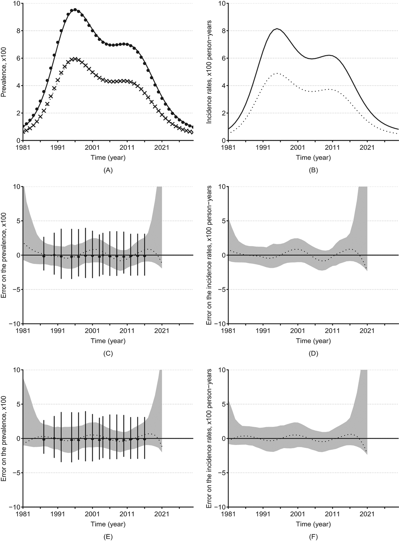
Simulated and estimated prevalence and incidence rate and their errors. Underlying prevalence (A) and incidence rates (B) in groups w (solid lines) and u (dotted lines). Absolute errors on the estimated prevalence and incidence by Model 1 ((C) and (D)) and by Model 2 ((E) and (F)) in group w. The dots and crosses in (A) represent the approximated prevalence in groups w and u, respectively; the dashed lines in (C), (D), (E) and (F) represent the median error on the estimates as a function of time, the greyed areas represent their 95 % confidence regions, and the vertical solid bars represent the 95 % confidence bars of the errors of the prevalence in simulated surveys.

It is unlikely that an investigator could guess the true model for this incidence based on the prevalence observed with noise. We assumed that prevalence studies were conducted in the population at times t = 7, 10, 12, 15, 17, 19, 21, 23, 24, 26, 28, 30, 32, 34, and 36. At each time, 250 individuals were surveyed in each sub-population and their infection statuses were sampled following binomial distributions with parameter puti or pwti,i=1…,15. We reconstructed the incidence and the prevalence using the simulated prevalence as described in Section 2.1. The process was repeated 1000 times. We set the maximum number of knots to 10 which corresponds to a model with 24 parameters, larger than the number of years when studies were conducted. At the first iteration, the best AIC was achieved for 3 knots (10 parameters) for both Models 1 and 2, corresponding to AIC of 3490.3 and 3490.9, respectively. For the subsequent iterations, we did not perform model selection; i. e. we estimated the parameters for the models selected at the first step. Figure 1 (C) and (E) show the errors on the estimated prevalence in group w by Models 1 and 2, respectively, while Figure 1 (D) and (F) display the errors on the estimated incidence, using the same models. The estimated incidence ratios where 0.61 (95 % CI: 0.51–0.73) and 0.59 (95 % CI: 0.49–0.72) for Models 1 and 2, respectively. Both approaches appeared to reconstruct both incidence and prevalence over time. The widths of the confidence intervals of the estimated curves were 37–76 % and 38–67 % shorter than those observed in surveys, for Models 1 and 2, respectively. For both models, the true curves appeared to be within the 95 % confidence region up to 7 before the first survey and 6 years after the last survey.

3.2 Real world data examples

The approaches described in Section 2 were used to estimate gonorrhea and syphilis prevalence and incidence trends in South Africa and Guinea-Bissau, respectively, setting the maximum number of knots to 10. We used data from the Spectrum’s global STI Data base described in [8]. That data base consists of a compilation of published adult gonorrhea, syphilis and chlamydia prevalence studies, surveys and routine Antenatal Care screening data [8, 25]. Briefly, South Africa’s gonorrhea data consisted of data from 39 studies conducted among pregnant women in antenatal care (ANC) between 2000 and 2011 in rural (27 studies) and/or urban (12) areas. Guinea-Bissau’s syphilis data came from 17 surveys conducted between 1990 and 2014 among police officers (14 studies) or among women attending ANC (3 studies). Data from each study consisted of the year the study was conducted, the observed prevalence, the sample size and the population type (rural or urban for gonorrhea and police officers or women attending ANC for syphilis). The median sample sizes were 475 (ranging from 85 to 4646) and 447 (ranging between 20 and 5666) for gonorrhea and syphilis, respectively. The prior bounds were set to c0=0, c1=0.2 and c2=0. Estimates of the duration of infections were D1=0.46 years and D2=4.13 years for gonorrhea and syphilis, respectively, corresponding to the WHO Afro-region duration estimates for those infections [1, 8]. These estimates were assumed to be constant over time and across population types; thus, the recovery rates were the inverse of these durations.

The bootstrap procedure was used for uncertainty analysis. We first applied the methods to the observed data. Then, at each bootstrap iteration, b = 1, …, 1000, the prevalence from each survey pij∗ (ij=1,…,Ij, j = 1, 2 indicate the survey type, Ij is the number of studies of type j) was sampled from the Beta distribution B(Nijpij0+1,Nij(1−pij0)+1), where Nij is the number of individuals sampled in study ij and pij0 is the prevalence estimated using the observed data. Finally, to account for uncertainty on the to the recovery rates (rj=1/Dj,j=1,2) estimates, we followed [10], i. e. we multiplied these estimates by a uniform distribution on the interval (0.5, 1.5).

The median of the bootstrap samples was reported as our estimate and the 2.5 % and 97.5 % percentiles were reported as the 95 % confidence limits.

3.2.1 Gonorrhea prevalence and incidence trends in South Africa

In the South Africa’s gonorrhea study, the smallest AIC were achieved with 6 knots (16 parameters) in both approaches. Model 2 provided the overall best model between the two classes explored (smallest AIC: 11406.2 vs 11422.7). That best model suggested the risk of gonorrhea acquisition of women in rural areas is 1.8 (95 % CI: 0.91–2.8) fold higher than that in urban areas. The resulting incidence and prevalence trends and their projections are displayed in Figure 2. This suggests that both the incidence and prevalence were likely to be decreasing in South Africa between 1998 and 2003 then increased until 2009 when another decline has started.

Figure 2:

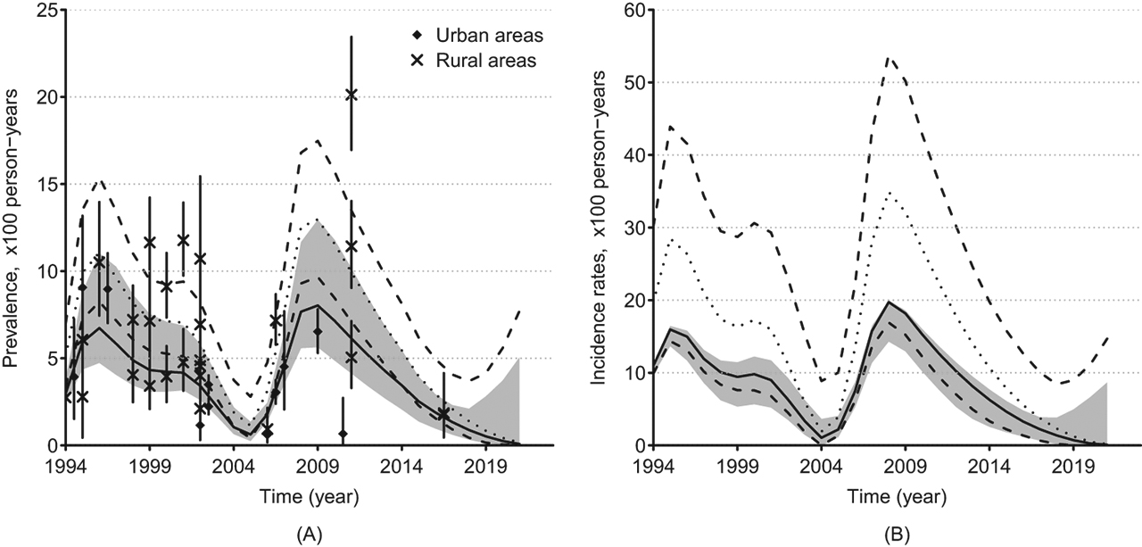
Gonorrhea Prevalence (A) and Incidence (B) rates in urban and rural areas of South Africa. The crosses and diamonds represent the observed prevalence among women attending antenatal care (ANC) in rural and urban areas, respectively. The solid lines represent prevalence and incidence estimates (50 th percentile) and the greyed areas represent the 95 % confidence regions in urban areas; the vertical solid bars represent the 95 % confidence bars of the prevalence observed in surveys. The dotted lines represent the 50 th percentile and the dashed lines represent the 2.5 and 97.5 ths percentiles of the estimates for women in rural areas as a function of time. The percentiles were obtained using the bootstrap resampling method.

3.2.2 Syphilis prevalence and incidence trends in Guinea-Bissau

The smallest AIC when considering Models 1 and 2 were achieved with 5 and 3 knots (14 and 10 parameters), respectively. Overall, the smallest AIC was 4820.3 and was obtained by the Model 2. Figure 3 (A) and (B) display the estimated prevalence and incidence trends of syphilis and their projections in Guinea-Bissau among both women attending ANC and police officers, using that model. It suggests that both incidence and prevalence declined from the early 2000’s to 2013, followed by a slow increase. Estimates of the incidence rate ratio suggest that syphilis incidence among police officers in Guinea-Bissau is 1.4 (95 % CI: 0.72–2.15) higher than the incidence in women attending ANC.

Figure 3:

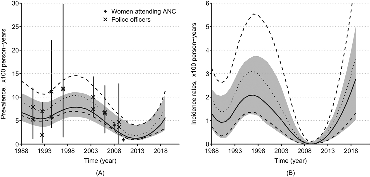
Syphilis Prevalence (A) and Incidence (B) rates in Guinea-Bissau. The crosses and diamonds represent observed prevalence among police officers and women attending antenatal care (ANC), respectively. The solid lines represent prevalence and incidence estimates (50 th percentile) and the greyed areas represent the 95 % confidence regions for ANC women; the vertical solid bars represent the 95 % confidence bars of the prevalence observed in surveys. The dotted lines represent the 50 th percentile and the dashed lines represent the 2.5 and 97.5 ths percentiles of the estimates for police officers as a function of time. The percentiles were obtained using the bootstrap resampling method.

4 Concluding remarks

We presented approaches to prevalence and incidence trends estimation of infections inducing negligible or no mortality, using second order segmented polynomials. The methods account for the process generating the prevalence over time in the population. These approaches were extended to handle covariates. Results from a simulation study showed that both approaches can work well, even when the incidence curve contains exponential components. The approaches were then applied a) to estimate gonorrhea prevalence and incidence trends among South Africa’s women in rural and urban areas and b) to estimate syphilis prevalence and incidence trends in women attending ANC and police officers Guinea-Bissau.

The two methods showed similar performance on simulated data. In the real data examples, however, the model deriving prevalence from incidence (Model 2) appeared to perform better than Model 1 as it provided smallest AIC. In terms of numerical cost, the latter model also appeared to perform better since it avoids calculation of some integrals. This suggests that Model 1 can only be preferred when the prevalence time series is long enough.

Our smoothing approaches have the advantage over classical splines for this specific problem, because they allow handling quadratic constraints on both the incidence and prevalence easily and determine the optimal number and position of knots automatically. In the simulation study, both models were able to reconstruct the history of the simulated epidemic which had two outbreaks with different magnitudes. This result can be justified by the fact that the class of candidate functions considered is relatively broad, what we believe, also confers good asymptotic properties to the proposed approaches. This suggests that the method can be extended to other infections, including infections with periodic patterns such as influenza.

Our study has some limitations. We assumed that recovery rates were constant over time, in our real data examples. That assumption was dictated by the availability of data; it is possible that the duration of the infections considered changed over time due to advances in treatment access, quality, uptake and availability of medicines. As shown in our simulation study, this limitation is not inherent to our models. Our models are simplistic in that they are agnostic regarding age and the dynamics between risk groups or key populations. Data on age patterns and drivers and key groups for STI are generally scarce, but for settings where these are available, our models could be refined to consider those, which would further help to understand the spread of the infections and develop suitable targeted intervention strategies. Refinement to include at least age patterns is envisioned, as forthcoming age-differentiated survey data may make this relevant.

Meanwhile, the methods presented can already use information collected from various sources and the likelihood functions can be adapted and the models used when individual data are available. The approach can work with and without covariates. One attractive feature of the extension to covariates is the possibility of adding random effects to account for heterogeneity. Moreover, covariates can help borrowing trends from other sources. For example, population-based gonorrhea prevalence data are generally sparse, but when routine clinical case reports data are available, these can be used to inform the trend in prevalence. In fact, one can model prevalence and case report data jointly, assuming for example that case report data follow a non-homogeneous Poisson process, and model the prevalence using the binomial model as done in this paper.

Finally, the methods presented in this paper can be generalized to any problem where the function to be estimated should lay in a domain with quadratic boundaries.

Acknowledgement

This work was supported by the WHO Reproductive Health and Research Department (Dr. Teordora Wi and Dr. Melanie Taylor) and Bill and Melinda Gates Foundation. The authors would like to thank John Stover for his interest in this work.

Appendix

A Proof that (3) is a solution to (2)

Let us assume that the functions i and r introduced in Section 2 are integrable. We first note that, from Lebesgue’s differentiation Theorem, we have:

ddt∫t0ti(u)+r(u)du=i(t)+r(t), for all t.

Thus

(17)ddtexp−∫t0ti(u)+r(u)du=i(t)+r(t)exp−∫t0ti(u)+r(u)du, for all t.

We also have:

ddt∫t0ti(u)exp−∫t0ti(s)+r(s)dsdu=i(t)+∫t0ti(u)ddtexp−∫t0ti(s)+r(s)dsdu.

i. e. using (17):

(18)ddt∫t0ti(u)exp−∫t0ti(s)+r(s)dsdu=i(t)−i(t)+r(t)∫t0ti(u)exp−∫t0ti(s)+r(s)dsdu, for all t.

Now, if we take the derivative of p given by (3) and use (17) and (18), we obtain:

ddtp(t)=i(t)−i(t)+r(t)p(t), for all t

which is equivalent to (2). One can derive (3) by solving (2) using the method of variation of constants.

B Gradient functions of the prevalence for Models 1 and 2

B.1 Gradient for functions in M

Let f∈M. Thus there exists m∈N such that f∈Mm. And we have, for all x ∈ (0, 1):

∂f(t)∂α0=1;∂f(t)∂h0=t;∂f(t)∂γl=hl(2(t−tk)−hl)ift∈(tk,tk+1)withk>lt2ift∈(tl,tl+1)0ift∈(tk,tk+1)withk<l

and, if m≥1, for l≥1

∂f(t)∂hl=2(γl−γk)(t−tk)+2∑j=l+1k−1(γl−γj)hjift∈(tk,tk+1)withk>l0ift∈(tk,tk+1)withk≤l.

For any smooth function g, the derivatives of g of may be obtained using the chain rule.

B.2 Gradient for prevalence function in Model 2

Let pm=ϕ(im), where i∈Mm and φ is the operator defined by (3). We can obtain partial derivatives of p using the formulas in the previous section and Fubini’s theorem:

(19)∂p(t)∂x=∂p(t0)∂x−p(t0)∫t0t∂i(u)∂xduexp−∫t0ti(u)+r(u)du+∫t0t∂i(u)∂x−i(u)∫ut∂i(s)∂xdsexp−∫uti(s)+r(s)dsdu

for x=α0,h0,γ0,h1,γ1,…,hm,γm. Formula similar to (15) can be used to approximate the derivatives given by (19). This is faster than using numerical derivative since the same grid can be used and the function u→exp−∫uti(s)+r(s)ds evaluated at the grid points once.

C Closed form for C and C1

Let pm∈M and c > 0. In order to calculate C(pm,c) as defined in Section 2.2.1, it is sufficient to know how to calculate C1(t)=∫0tmax(p(s),0)ds, where p is a second order polynomial on (0, 1). Let p be a second order polynomial on (0, 1). Thus there exists α,β,γ∈R3 such that for all s ∈ (0, 1), p(s)=α+βs+γs2. Let C0(t)=∫0tp(s)ds=αt+12βt+13γt3; we have:

If γ = 0
1. If α≥0 and β≥0, then C1(t)=C0(t);
2. If α≥0 and β < 0, then let t˜0=−αβ
  1. If t≤t˜0, C1(t)=C0(t);
  2. If t≥t˜0, C1(t)=C0(t˜0);
3. If α≤0 and β≤0, then C1(t)=0
4. If α≤0 and β > 0, then let t˜0=−αβ
  1. If t≤t˜0, C1(t)=0;
  2. If t≥t˜0, C1(t)=C0(t)−C0(t˜0);
If γ≠0, let Δ=β2−4αγ
1. If Δ≤0
  1. If γ < 0, C1(t)=0
  2. If γ > 0, C1(t)=C0(t)
2. If Δ > 0, let t˜01=−β+Δ2γ, t˜02=−β−Δ2γ and t1˜=mint˜01,t˜02, t2˜=maxt˜01,t˜02
  1. If γ > 0
    If t˜2≥0, C1(t)=C0(t)
    If t≤t˜1 and t˜2>0, then C1(t)=C0(t)
    If t>t˜1, t≤t˜2, and t˜2>0, then
    if t˜1>0, C1(t)=C0(t˜1)
    if t˜1≤0, C1(t)=0
    If t>t˜2 and t˜2>0, then C1(t)=C0(t)−C0(t˜2)
  2. If γ < 0
    If t˜2≥0 then C1(t)=0;
    If t≤t˜1 and t˜2>0, then C1(t)=0;
    If t>t˜1, t≤t˜2, and t˜2>0, then
    if t˜1≤0 then C1(t)=C0(t˜1)
    if t˜1>0 then C1(t)=C0(t)−C0(t˜1)
    If t>t˜2 and t˜2>0, then
    if t˜1≤0 then C1(t)=C0(t˜2)
    if t˜1>0 then C1(t)=C0(t˜2)−C0(t˜1)

Similar approach can be used to evaluate C1.

References

[1] Newman L, Rowley J, Vander Hoorn S, Wijesooriya NS, Unemo M, Low N, et al. Global estimates of the prevalence and incidence of four curable sexually transmitted infections in 2012 based on systematic review and global reporting. PloS One. 2015;10:e0143304.10.1371/journal.pone.0143304Suche in Google Scholar PubMed PubMed Central

[2] Gerbase AC, Rowley JT, Heymann DH, Berkley SF, Piot P. Global prevalence and incidence estimates of selected curable stds. Sex Transm Infect. 1998;74:S12–6.Suche in Google Scholar

[3] Ahmadi-Abhari S, Guzman-Castillo M, Bandosz P, Shipley MJ, Muniz-Terrera G, Singh-Manoux A, et al. Temporal trend in dementia incidence since 2002 and projections for prevalence in england and wales to 2040: modelling study. BMJ (Clinical Research ed.). 2017;358:j2856.10.1136/bmj.j2856Suche in Google Scholar PubMed PubMed Central

[4] Brinks R, Bardenheier BH, Hoyer A, Lin J, Landwehr S, Gregg EW. Development and demonstration of a state model for the estimation of incidence of partly undetected chronic diseases. BMC Med Res Methodol. 2015;15:98.10.1186/s12874-015-0094-ySuche in Google Scholar PubMed PubMed Central

[5] Leon L, Kasereka S, Barin F, Larsen C, Weill-Barillet L, Pascal X, et al. Age- and time-dependent prevalence and incidence of hepatitis c virus infection in drug users in france, 2004–2011: model-based estimation from two national cross-sectional serosurveys. Epidemiol Infect. 2017;145:895–907.10.1017/S0950268816002934Suche in Google Scholar PubMed

[6] Nogareda F, Le Strat Y, Villena I, De Valk H, Goulet V. Incidence and prevalence of toxoplasma gondii infection in women in france, 1980–2020: model-based estimation. Epidemiol Infect. 2014;142:1661–70.10.1017/S0950268813002756Suche in Google Scholar PubMed

[7] Tan T, Chen L, Liu F. Model of multiple seasonal autoregressive integrated moving average model and its application in prediction of the hand-foot-mouth disease incidence in changsha. Zhong nan da xue xue bao. Yi xue ban. 2014;39:1170–6.Suche in Google Scholar

[8] Korenromp EL, Mahiané G, Rowley J, Nagelkerke N, Abu-Raddad L, Ndowa F, et al. Estimating prevalence trends in adult gonorrhoea and syphilis in low- and middle-income countries with the Spectrum-STI model: results for Zimbabwe and Morocco from 1995 to 2016. Sex Transm Infect. 2017;93:599–606. doi: 10.1136/sextrans-2016-052953.Suche in Google Scholar PubMed PubMed Central

[9] Badrakh J, Zayasaikhan S, Jagdagsuren D, Enkhbat E, Jadambaa N, Munkhbaatar S, et al. Trends in adult chlamydia and gonorrhoea prevalence, incidence and urethral discharge case reporting in mongolia from 1995 to 2016–estimates using the spectrum-sti model. West Pac Surveillance Response J. 2017;8:20.10.5365/wpsar.2017.8.2.007Suche in Google Scholar PubMed PubMed Central

[10] Bennani A, El-Kettani A, Hançali A, El-Rhilani H, Alami K, Youbi M, et al. The prevalence and incidence of active syphilis in women in Morocco, 1995–2016: model-based estimation and implications for STI surveillance. PLoS ONE. 2017;12:e0181498. DOI:10.1371/journal.pone.0181498.Suche in Google Scholar

[11] El-Kettani A, Mahiané G, Bennani A, Abu-Raddad L, Smolak A, Rowley J, et al. Trends in adult chlamydia and gonorrhea prevalence, incidence and urethral discharge case reporting in morocco over 1995–2015 estimates using the spectrum-sexually transmitted infection model. Sex Transm Dis. 2017;44:557.10.1097/OLQ.0000000000000647Suche in Google Scholar PubMed PubMed Central

[12] Enkhbat E, Korenromp EL, Badrakh J, Zayasaikhan S, Baya P, Orgiokhuu E, et al. Adult female syphilis prevalence, congenital syphilis case incidence and adverse birth outcomes, mongolia 2000–2016: Estimates using the spectrum sti tool. Infect Dis Modell. 2018;3:13–22.10.1016/j.idm.2018.03.003Suche in Google Scholar PubMed PubMed Central

[13] Holmes KK, Sparling PF, Mardh PA, Lemon SM, Stamm WE, Piot P, et al. Sexually transmitted diseases. New York City: McGraw-Hill Co., 1999;479–85.Suche in Google Scholar

[14] Brinks R, Landwehr S. Change rates and prevalence of a dichotomous variable: simulations and applications. PLoS One. 2015;10:e0118955.10.1371/journal.pone.0118955Suche in Google Scholar

[15] Mahiane GS, Ouifki R, Brand H, Delva W, Welte A. A general hiv incidence inference scheme based on likelihood of individual level data and a population renewal equation. PloS One. 2012;7:e44377.10.1371/journal.pone.0044377Suche in Google Scholar

[16] Brookmeyer R, Laeyendecker O, Donnell D, Eshleman SH. Cross-sectional hiv incidence estimation in hiv prevention research. J Acquired Immune Deficiency Syndromes (1999). 2013;63:S233.10.1097/QAI.0b013e3182986fdfSuche in Google Scholar

[17] Freeman J, Hutchison GB. Prevalence, incidence and duration. Am J Epidemiol. 1980;112:707–23.10.1093/oxfordjournals.aje.a113043Suche in Google Scholar

[18] Mahiané SG, Laeyendecker O. Segmented polynomials for incidence rate estimation from prevalence data. Stat Med. 2017;36:334–44.10.1002/sim.7130Suche in Google Scholar

[19] Li DH, Fukushima M. A modified bfgs method and its global convergence in nonconvex minimization. J Comput Appl Math. 2001;129:15–35.10.1016/S0377-0427(00)00540-9Suche in Google Scholar

[20] Brinkhuis J, Protassov V. The lagrange multiplier rule revisited. Technical report, Econometric Institute Research Papers. 2008.Suche in Google Scholar

[21] Biswas B, Chatterjee S, Mukherjee S, Pal S. A discussion on euler method: A review. Electron J Math Anal Appl. 2013;1:294–317.Suche in Google Scholar

[22] Avenir Health. Spectrum. Avenir health, Glastonbury, CT, USA, 2017. http://www.avenirhealth.org/software-spectrum.php.Suche in Google Scholar

[23] R Core Team. R: A language and environment for statistical computing. R foundation for statistical computing. Vienna, Austria, 2017. https://www.R-project.org/.Suche in Google Scholar

[24] Kenyon CR, Osbak K, Tsoumanis A. The global epidemiology of syphilis in the past century - a systematic review based on antenatal syphilis prevalence. PLoS Negl Trop Dis. 2016;10:e0004711.10.1371/journal.pntd.0004711Suche in Google Scholar PubMed PubMed Central

[25] Chico RM, Mayaud P, Ariti C, Mabey D, Ronsmans C, Chandramohan D. Prevalence of malaria and sexually transmitted and reproductive tract infections in pregnancy in sub-saharan africa: a systematic review. JAMA, 2012;307:2079–86.10.1001/jama.2012.3428Suche in Google Scholar PubMed

Received: 2017-09-12

Revised: 2018-12-18

Accepted: 2019-04-10

Published Online: 2019-06-08

Artikel in diesem Heft

https://doi.org/10.1515/ijb-2017-0073

Schlagwörter für diesen Artikel

incidence rate; prevalence; segmented polynomials; maximum likelihood estimation; model selection