Modelling Mixed Types of Outcomes in Additive Genetic Models

1 Introduction

Linear mixed effects models [1, 2] are the main statistical tool in the context of quantitative genetic data analysis. The estimation of the additive genetic variance and thus the heritability of different outcomes is one of the main goals in quantitative genetic [3, 4]. Examples appear frequently in evolutionary biology [5] and animal breeding [6]. Although flexible for Gaussian data, linear mixed effects models are unsuitable for analysing binary, binomial, count and asymmetric continuous outcomes.

For the analysis of non-Gaussian outcomes the generalized linear mixed models (GLMMs) framework is a frequent choice [7, 8]. GLMMs consist of specifying a generalized linear model conditionally on a multivariate latent distribution, often the multivariate Gaussian. In general GLMMs are computationally demanding and many different algorithms have been proposed in the past three decades, see [9] and [10] for additional references. A further aspect of GLMMs that gives rise to concern is the general lack of a closed-form expression for the likelihood and the marginal distribution of the data vector. A related question is the special interpretation of parameters inherent from the construction of GLMMs. Thus, the covariate effects are conditional on the latent variables, whereas the correlation structure is marginal for the latent variables rather than for the outcomes.

The literature to deal with mixed types of outcomes in the context of quantitative genetic is sparse. [7, 11] proposed to use the GLMMs family relying on MCMC (Markov Chain Monte Carlo) methods for estimation in the Bayesian framework. MCMC methods for GLMMs are challenging in terms of convergence and computational time. Furthermore, these challenges seem to be amplified for mixed types of outcomes and covariance modelling using genetic structures. Moreover, the implementation itself can be difficult, especially for end-users who might not be expert in programming. For a more comprehensive discussion on the computational challenges for MCMC methods, we refer the interested reader to [12] and [10]. [13] presented the penalized multivariate linear mixed model for the analysis of multi-traits in the context of genome-wide association studies. For a recent application of this approach and further discussion about mixed types of outcomes, see [14].

The computation of the heritability index in the Gaussian case is trivially defined by the proportion of the variance attributed to the genetic component. For non-Gaussian data, it is not immediately obvious how to define the heritability of an outcome. A comprehensive discussion about the computation of the heritability index for non-Gaussian data based on GLMMs is presented in [15] along with a proposal of solution. Although, this new development on the computing of the heritability index for non-Gaussian data, it remains a daunting task requiring intricate calculation involving multivariate integrals and specific algorithms.

In this paper, we present an alternative approach for modelling mixed types of outcomes in the context of genetic data based on the multivariate covariance generalized linear models (McGLMs) [16].

In the McGLM framework the marginal covariance matrix is explicitly modelled combining a matrix linear predictor and a covariance link function. Variance function are employed to take into account non-normality and the mean structure is modelled using a link function and a linear predictor. McGLMs are fitted using quasi-likelihood and Pearson estimating functions, based on second-moment assumptions, and implemented in an efficient Newton scoring algorithm. McGLMs are an extension of the linear mixed effects models to deal with multivariate non-Gaussian data and have the last one as a special case. Furthermore, from the marginal specification of McGLMs emerges a marginal measure of heritability for non-Gaussian data.

McGLMs have many in common with GEE (Generalized Estimating Equations) models popular in the analysis of longitudinal data [17]. However, McGLMs were explicitly designed to deal with multiple outcomes and allow for a flexible and interpretable specification of the marginal covariance structure using a covariance link function combined with a linear combination of known matrices. Furthermore, in the McGLM framework the dispersion parameters play an important role in terms of model specification and interpretation. On the other hand, current GEE implementations deal only with one outcome and include a short list of pre-specified covariance structures, such as auto-regression and compound symmetry [18, 19]. In general in the GEE framework the dispersion parameters are considered as nuisance. In terms of fitting algorithm, both methodologies use the quasi-score function for estimation of the regression coefficients. In the McGLM framework the dispersion parameters are estimated using the Pearson estimating function [20], while in the GEE context the method of moments and the GEE2 are frequent choices [21, 22].

The model we shall present in Section 3 is motivated by the data set analysed in [8] consisting of a natural meta population of house sparrow (Passer domesticus) on six islands off the coast of Helgeland, Northern Norway. In this study blood samples were used to determine genetic parenthood, and the genetic pedigree for the birds could be established. The outcomes of interest are: (1) bill depth, (2) breeding season success, and (3) average reproductive intensity. The main biological goals are to compute the heritability of the different outcomes, as well as the possible correlation between outcomes that can be due to genetic and environment effects. This example is particularly interesting because the outcomes are of mixed types, i.e. bill depth is a continuous outcome, while breeding season success and average reproductive intensity are examples of binomial and count outcomes.

In view of the recent developments in the McGLMs framework the main contributions of this article are: (i) introducing a suitable specification of the McGLMs to deal with mixed types of outcomes in the context of genetic data analysis. (ii) presenting the extended binomial variance function for handling binomial and restricted outcomes. (iii) proposing a new marginal measure of heritability for non-Gaussian data. (iv) presenting a comparison between the conditional specification of GLMMs and the marginal specification of McGLMs to explain why negative heritability index can appear in practical data analysis and how to use this fact to easily assess the significance of the genetic effects. (v) adapting the NORTA (Normal to anything) [23] algorithm for simulation of McGLMs. (vi) presenting a simulation study to check the asymptotic properties of the estimating function estimators with emphasis to the correlation between outcomes and the new measure of heritability and (vii) analysing the house sparrow data set comparing the results with the ones obtained by [8].

We present the data set in Section 2. Section 3 presents the model and discusses its properties. Section 6 compares the conditional and marginal model specifications and explains why negative heritability index appears naturally in the marginal specification. Section 5 adapts the NORTA algorithm for simulation of McGLMs. Section 6 presents a simulation study to verify the asymptotic properties of the estimating function estimators. Section 7 presents the application of the model to the data. Finally, the main results are discussed in Section 8, including some directions for future investigations. The data set and R [24] code are available in the supplementary material.

2 Data set

The case study analysed in this paper uses data from a natural meta population of house sparrow (Passer domesticus) on six islands off the coast of Helgeland, Northern Norway. For additional description of the field work, study area and genetic parenthood analyses, see [5, 8, 25, 26].

In this study, blood samples were used to determine genetic parenthood, and a genetic pedigree for the birds could be established. We highlight that the genetic parenthood structure was determined for each bird. The study has three outcomes of interest: (1) bill depth (BD), (2) breeding season success (BS), and (3) average reproductive intensity (AR). There are three covariates, namely sex (sex), hatch year (HY) and hatch island (HI). The data set that we have access corresponds to the study period from 1993 to 2002, which corresponds to 950 observations. Histograms in Figure 1 suggest that the Gaussian and binomial distributions are suitable choices for BD and BS. While hinting at potential problems with excess of zeroes and overdispersion for AR. The scatter plots suggest correlation only between AR and BS. It is important to highlight that the plots presented in Figure 1 can detect only marginal correlations between the traits and do not take into account the origin, genetic or environment as well as the covariate effects.

Figure 1:

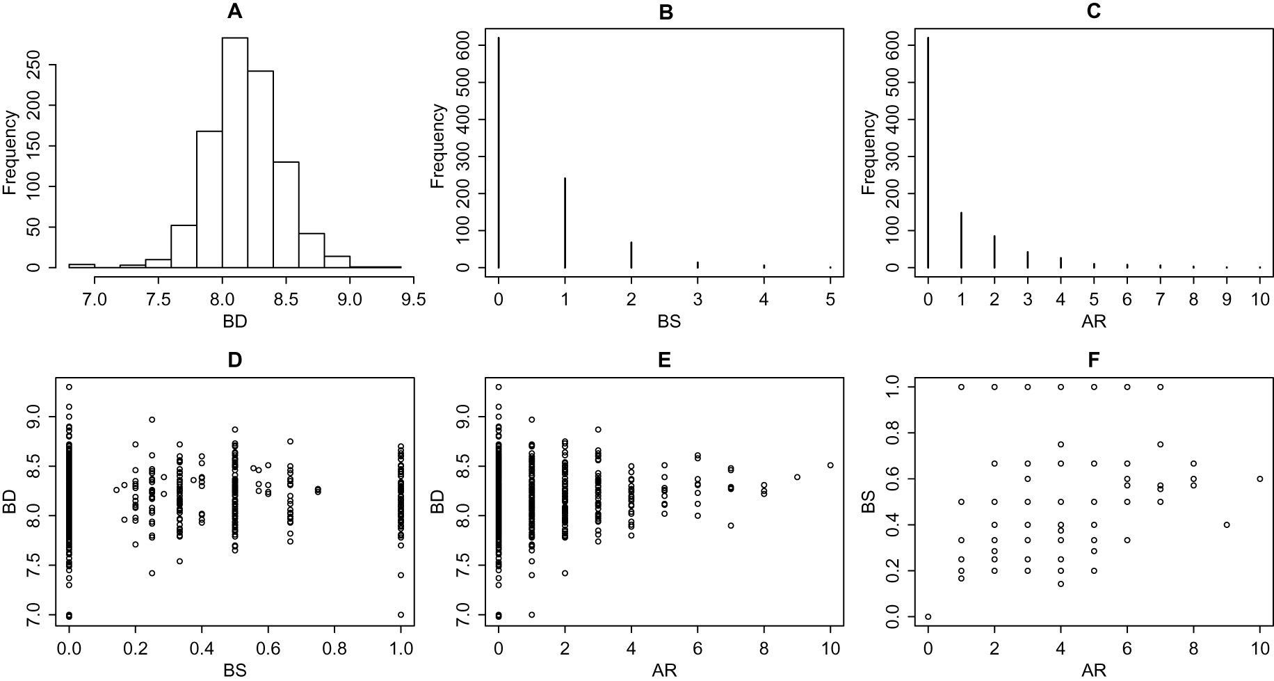
Histograms (A to C) and scatter plots (D to F) for outcomes in the house sparrow data set.

[8] analysed the house sparrow data set using univariate GLMMs in the Bayesian framework with random effects specified on the bird level. The INLA (Integrated Nested Laplace Approximation) algorithm [12] was employed for fitting the models. For the outcome BD the authors assumed a Gaussian distribution, while for BS and AR their choices were the binomial and zero-inflated Poisson distributions, respectively. The deviance information criterion (DIC) was applied for model selection. In the Section 7, we compare the results obtained by [8] with the ones obtained by fitting the multivariate model that we shall present in Section 3.

3 McGLMs for mixed types of outcomes

Let YN×R={Y1,…,YR} be an outcome matrix and let MN×R={μ1,…,μR} denote the corresponding matrix of expected values. Let Σr denote the N×N covariance matrix within the outcome r for r=1,…,R. Similarly, let Σb be the R×R correlation matrix between outcomes. The McGLM as proposed by [16] is given by

where

is the generalized Kronecker product [27]. The matrix Σ˜r denotes the lower triangular matrix of the Cholesky decomposition of Σr. The operator Bdiag denotes a block diagonal matrix and I denotes an N×N identity matrix. The functions gr are orthodox link functions. Let Xr denote an N×kr design matrix and βr a kr×1 regression parameter vector.

The key point for specifying McGLMs for mixed types of outcomes is the specification of the covariance matrix within outcomes Σr. Following [16] we define the covariance within outcomes by

where V(μr;pr)=diag(ϑ(μr;pr)), denotes a diagonal matrix, whose main entries are given by the variance function ϑ(⋅;pr) applied element wise to the vector μr. The variance function plays an important role in McGLMs, since different choices for ϑ(⋅;pr) imply different marginal outcome distributions.

In the house sparrow data set, we have three types of outcomes, namely, a continuous (BD), a binomial (BS) and a count (AR). To take into account the nature of the outcomes, in this paper, we adopted three set of variance functions. To deal with continuous outcomes the power variance function ϑ(⋅;pr)=μrpr provides a flexible family of models, since it describes the Tweedie family of distributions that has as special cases the Gaussian (p=0), Gamma (p=2) and inverse Gaussian (p=3) distributions [28, 29, 30].

For handling binomial data we propose to use the extended binomial variance function defined by ϑ(⋅;pr)=μrpr1(1−μr)pr2 where we introduced two new extra power parameters in order to become the orthodox binomial variance function more flexible. This variance function can also deal with bounded outcomes, as proportions or indexes. An interesting special case of the extended binomial variance function, is p1=p2=3 that corresponding to the Simplex distribution [31]. However, we highlight that such variance function is not suitable for binary outcomes.

Finally, for modelling count outcomes we following [32] adopted the Poisson-Tweedie dispersion function [33], i.e. \-ϑ(⋅;p)=μ+τμp, where τ is the dispersion parameter. We highlight that the dispersion function introduced by [33] is not a variance function in the sense of [30], but for practical data analysis both are completely analogous. In that case the covariance within outcomes takes the special form,

where V(μr;pr)=diag(μrpr), is a diagonal matrix whose main entries are given by the power variance function. The Poisson-Tweedie family of distributions provide a rich class of models to deal with count outcomes, since many important distributions appear as special cases, examples include the Hermite (p=0), Neyman Type A (p=1), negative binomial (p=2) and Poisson-inverse Gaussian (p=3).

The power parameter p plays an important role in the context of McGLMs for mixed types of outcomes, since for all variance functions discussed it is an index which distinguishes between important distributions. The algorithm proposed by [16] and implemented in the R package mcglm [34] allows us to estimate the power parameter, which works as an automatic distribution selection.

The dispersion matrix Ω(τr) describes the part of the covariance within outcomes that does not depend on the mean structure. Based on the ideas of [35] and [36] [16] proposed to model the dispersion matrix using a matrix linear predictor combined with a covariance link function, i.e.

where h is the covariance link function, Zrd with d=0,…,D are known matrices reflecting the covariance structure within the response variable r, and τr=(τr0,…,τrD) is a (D+1)×1 vector of dispersion parameters.

McGLMs are fitted using an efficient Newton scoring algorithm based on quasi-likelihood and Pearson estimating functions, using only second-moment assumptions. The algorithm is described in detail by [16] and implemented in the mcglm [34] package for the R statistical software. The data set and R code are available in the supplementary material.

4 Conditional and marginal models: Explaining negative heritability index

McGLMs introduce the additive genetic effects directly in the marginal covariance matrix by using a linear combination of known matrices, see eq. (3). It is in contrast to the more orthodox approach based on hierarchical models, where the additive genetic effects are introduced through random effects using a conditional specification, see for example [2] and [11]. In this section, we discuss conditional and marginal model specifications in the context of additive genetic models and explain why negative heritability index appears naturally in the marginal specification. Furthermore, we use this fact to explain how to assess the significance of the genetic effects. To simplify the discussion and without loss of generality consider the one outcome case, i.e R=1. Thus, the outcome matrix takes the form YN×1. An often approach to model genetic data is to assume a hierarchical model as follows:

It is assumed that the components of Y are conditionally independent given additive genetic effects Z and distributed as f(⋅;μ,τ0). The additive genetic effects are assumed f∗ distributed, where f∗ represents a multivariate distribution with vector of expected values 0 and covariance matrix τ1A. The parameters τ0>0 and τ1>0 are dispersion parameters associated with the environmental and genetic effects, respectively. The linear predictor is linked to the mean, μ by a link function g and consists of the sum of fixed effects Xβ and additive genetic effects Z. The N×k design matrix X contains values of k covariates and β is a k×1 vector of regression parameters. The class of generalized linear mixed models is obtained from eq. (4) by assuming that f(⋅;μ,τ0) belongs to the exponential family of distributions and f∗(0,τ1A) is a multivariate Gaussian distribution. In this context, the parameters τ0 and τ1 are frequently called variance components.

The conditional specification eq. (6) makes clear that the dispersion parameters should be positive and provides a convenient interpretation of the statistical model components for quantitative genetic analysis. In this context, however, we are interested in testing whether or not the genetic additive effects are absent in the model, which in turn is equivalent to testing the dispersion parameter τ1 equals to zero. Note that, such a null hypothesis places the dispersion parameter on the boundary of the parameter space and commonly used tests, such as the likelihood ratio, Wald and score tests, do not have the traditional chi-squared distribution [40]. In spite of corrections for the test statistics are available [41, 42], it remains an inconvenient feature of the conditional specification. On the other hand, as we shall discuss below such inconvenient feature can be overcome by a marginal specification. In general, the marginal distribution of Y cannot be obtained in closed-form from the conditional specification. Moreover, the model parameters should be carefully interpreted, since the covariate effects are conditional on the additive genetic effects, whereas the covariance structure is marginal for the random effects rather than for the outcome.

A notorious special case of eq. (6) is the Gaussian linear mixed effects models obtained by assuming that f(⋅;μ,τ0) is Gaussian distributed and g as the identity link function. In that case is straightforward to show that the marginal distribution of Y is Gaussian with mean and variance given by

where it is clear that the only request to obtain a valid multivariate Gaussian distribution is that the covariance matrix Σ be positive definite. The parameter space of the dispersion parameters in the marginal model is the set Θ={τ0,τ1:Σ>0}, where Σ>0 means that Σ is a positive definite matrix. Furthermore, recall that a necessary condition for a matrix be positive definite is that the elements of its diagonal Σll>0,∀l,l=1,…,N. It implies that τ0Ill>−τ1All, which in turn shows that negative values at least at some extend are allowed for the parameter τ1. It is important to highlight that the condition Σll>0 is necessary, but not sufficient to Σ>0. The heritability index eq. (5) in that case takes the form h1=τ1/(τ0+τ1), which implies that when τ1<0 the heritability index is negative. In the marginal specification the parameter space is not trivially specified, but it has the advantage that the null hypotheses τ1=0 is not placed on the boundary of the parameter space and commonly used tests, such as the likelihood ratio, Wald and score tests can be applied without any additional corrections. In the cases where the additive genetic effects are non-significant, i.e. τ1=0 we expected that E(τˆ1)=0, where τˆ1 denotes an unbiased estimator of τ1. However, in practical data analysis is perfectly possible to observe realized values of τˆ1 smaller than zero, it is due to the sample variation, as usual when testing regression coefficients significance in the linear predictor. In the Section 6, as part of our simulation study, we assess the empirical distribution of τˆ1 and show that under the null hypothesis τ1=0 a simple Wald test can be used to test the significance of the additive genetic effects.

The McGLMs extend the Gaussian marginal specification eq. (7) to deal with non-Gaussian data by introducing link, variance and covariance link functions. In the case of one outcome and using the identity covariance link function, the general model eq. (1) customized to take into account the additive genetic effects has the following form

Hence, the terms of the diagonal matrix V(μ;p) are given by the variance function applied element wise to the vector μ, these values are always positive. Thus, the argument used to explain negative heritability index in the Gaussian case applies directly to the non-Gaussian case. Finally, by the properties of the generalized Kronecker product, if each marginal covariance matrix is positive definite, the joint covariance matrix is also positive definite. Finally, it is important to highlight that the McGLMs are specified based only on second-moments assumptions. Thus, the existence of a conditional model, a part of the Gaussian case, whose moments are given by eq. (1) remains an open question.

5 Simulation of McGLMs

In this section we adapt the NORTA algorithm for simulation of McGLMs with mixed types of outcomes. The NORTA algorithm described in detail by [23] is a simple, but still powerful method for simulation of random vectors with arbitrary marginal distributions and pre-specified correlation matrix. The key idea behind the NORTA method is to transform a multivariate Gaussian random vector into the desired random vector.

To simplify the notation, let Y=(Y1⊤,…,YR⊤)⊤ denote the NR×1 stacked vector of the outcome matrix YN×R by columns. The goal is to simulate a random vector Y whose components {Y1,…,YNR} have arbitrary marginal distributions denoted by FYl for l=1,…,NR and covariance matrix Var(Y)=C. Here, FYl denotes an arbitrary cumulative distribution function (cdf). Without loss of generality, suppose that C is a correlation matrix. Let Y represent a transformation of an NR-dimensional standard multivariate Gaussian vector Z={Z1,…,ZNR}⊤ with correlation matrix CZ. The NORTA vector is given by

where Φ[⋅] is the univariate standard Gaussian cdf applied element-wise to the vector Z and FYl−1(u)≡inf{y:FYl(y)≥u} denotes the inverse cdf. As point out by [23] the transformation FYl−1(Φ[⋅]) ensures that Yl has the desired marginal distribution FYl. Thus, the central problem is to specify the correlation matrix CZ in a such way that the vector Y has the desired correlation matrix C. Note that, the marginal variance can be controlled by the marginal distribution FYl, so the specification in terms of correlation matrix does not imply any loss of generality.

Let Yl and Yl′ denote the elements l and l′ of the vector Y, respectively. For l≠l′, let ρZ(l,l′) be the (l,l′)th element of CZ, and let ρY(l,l′) be the (l,l′)th element of C. The correlation matrix of Z directly determines the correlation matrix of Y, since

for all l≠l′. The correlation is defined by

where the marginal quantities E(Yl), E(Yl′), Var(Yl) and Var(Yl′) are defined by FYl and FYl′. The idea is to adjust the correlation matrix CZ to obtain the desired correlation matrix C of Y. In eq. (8) is clear that we can keep attention on the E(YlYl′) term. Recall that (Zl,Zl′) has a standard bivariate Gaussian distribution. Thus,

where Φ(zl,zl′) denotes a standard bivariate Gaussian probability density function with correlation ρZ(l,l′). We restrict our attention in distributions for which the integral eq. (9) exists. In general the integral eq. (9) has no closed form, thus we adopted the Retrospective Approximation algorithm [43] implemented in the R package NORTARA [44]. Note that, the problem of determining CZ that provides the desired correlation matrix C for Y reduces to NR(NR−1)/2 independent problems. For large data sets the problem becomes time consuming. However, we noted that for many situations the correlation ρZ(l,l′) is not far away of the correlation ρY(l,l′). Thus, we can solve the integral eq. (9) for a grid of values of ρY(l,l′) and apply a linear regression model to interpolate all values of ρY(l,l′) required to build the matrix C.

6 Simulation study

In this section we present a simulation study to verify the properties of the estimating function estimators. We considered a mixed types of outcomes scenario where a combination of Gaussian, binomial and Poisson outcomes is observed. The matrix linear predictor for each outcome was specified by a linear combination of an identity matrix and a relatedness matrix defined by a pedigree structure, see eq. (3). The R packages pedigree[45] and nadiv were employed to simulate the pedigree structure and build the relatedness matrix, respectively. The simulated pedigree consists of ten independent families, each one with five generations and an increasing number of individuals. We considered 5, 10 and 20 individuals per family, resulting in sample of sizes 250, 500 and 1000.

In this simulation study, we focus on the estimation of the correlation between outcomes and the new heritability index. We designed five simulation scenarios in order to explore the range of values of the heritability index. The first scenario considered a negative heritabililty index, thus we fixed the dispersion parameter values at (τr0=1.2,τr1=−0.1) which implies that hr1=−0.090. Since, the values of the main diagonal of the relatedness matrix A are always positive and in general close to 1 more extreme negative values will generate improper models, i.e. Σ is not positive definite. It is important to highlight that this scenario is challenge, since the dispersion parameter τr1 is close to the boundary of the parameter space. The second scenario considered the case of non-significant additive genetic effects, i.e. (τr0=1,τr1=0) which implies that the heritability index is zero. This scenario is interesting, since it allows us to study the empirical distribution of hr1 under the null hypotheses τr1=0, see the discussion in Section 4. Finally, for the other three scenarios, we considered the parameters (τr0=0.75,τr1=0.25), (τr0=0.5,τr1=0.5) and (τr0=0.25,τr1=0.75), respectively. Thus, the heritability index presents the values 0.25,0.5 and 0.75, respectively.

For all simulation scenarios, the correlations between outcomes were specified as ρ12=0.8, ρ13=0.6 and ρ23=0.4, where ρ12 denotes the correlation between the Gaussian and binomial marginals, similarly ρ13 and ρ23 denote the correlation between the Gaussian and Poisson marginals and between the binomial and Poisson marginals, respectively.

The Gaussian, binomial and Poisson scenarios consider linear predictors with intercepts and slopes given by: (β10=10,β11=2), (β20=5,β21=0.2) and (β30=0.5,β31=0.6). The covariate is a sequence from −2 to 2 and length equals the sample size. The values of the regression coefficients and the covariate were chosen in order to explore a large part of the support of each marginal distribution.

The Gaussian marginal was modelled using the identity link function and constant variance function. For the binomial marginal we adopted the logit link function and the orthodox binomial variance function. Finally, the Poisson marginal was modelled using the log link function and the Tweedie variance function with power parameter fixed at 1. For all outcomes the identity covariance link function was adopted.

For each simulation scenario, we generated 500 data sets to evaluate the bias, consistency and coverage rate of the estimating function estimators. Figure 2 shows the average bias plus and minus the average standard error for the correlation and heritability parameter estimators for each scenario. The scales are standardized for each parameter dividing the average bias and the limits of the confidence intervals by the standard error obtained on the sample of size 250.

Figure 2:

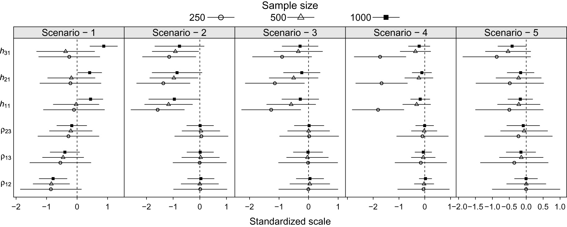
Average bias and confidence interval on a standardized scale by scenarios and sample sizes for the correlation and heritability parameter estimators.

Figure 2 shows that for the scenarios 2 to 5 the estimating function estimators for the correlation parameters between outcomes are unbiased and consistent. For the scenario 1 the correlation between the Gaussian and binomial marginals (ρ12) is underestimated. Although, the bias is small in its magnitude and decreases while the sample size increases.

The heritability index is underestimated in the scenarios 2 to 5 and small sample size. However, in general the bias decreases to zero while the sample size increases, as expected. On the other hand, in the scenario 1 the heritability index is well estimated for small samples, but for large sample the bias increases. The standard errors for all estimators decrease while the sample size increases, showing the consistency of the estimating function estimators.

In order to further investigate the origin of the underestimation of the heritability index Figure 3 presents the average bias plus and minus the average standard error on standardized scale for the dispersion parameter estimators for each simulation scenario.

Figure 3:

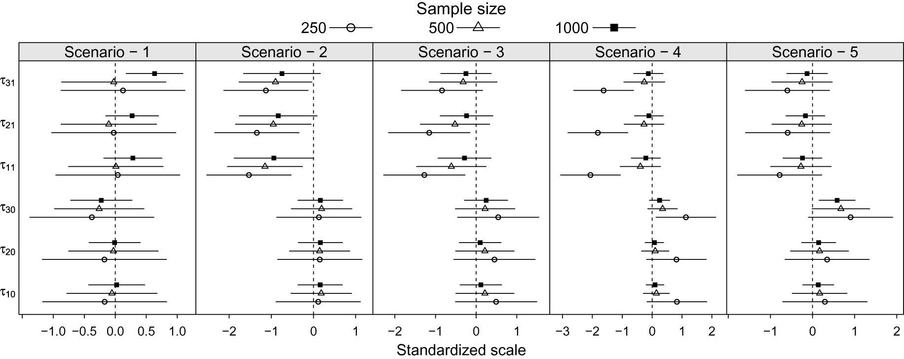
Average bias and confidence interval on a standardized scale by scenarios and sample sizes for the dispersion parameter estimators.

The results presented in Figure 3 show that in the scenarios 3 to 5 the dispersion parameters associated with the environmental effects are overestimated for small samples, while the dispersion parameters associated with the additive genetic effects are underestimated. These results explain the underestimation of the heritability index detected in the Figure 2. The scenario 1 presents a different situation, where the dispersion parameters associated with the environmental effects are slightly underestimated and the ones associated with the genetic effects are slightly overestimated. Similarly, we have seen in Figure 2 the bias associated with the parameters τ11,τ21 and τ31 increases for large samples in the scenario 1.

The simulation scenario 2 shows that the dispersion parameters associated with the additive genetic effects are underestimated, even for large samples. This result shows that in practice when the additive genetic effects are non-significant, i.e. τr1=0 we still can observe negative values for τˆr1 and consequently for the heritability index. Such results should be interpreted carefully and accompanied of the standard error associated with both the dispersion and heritability parameter estimators. The estimating function approach used to fit McGLMs provides asymptotic standard errors that can be used to construct confidence intervals as well as Wald statistics test. To check the accuracy of such standard errors Figure 4 presents the coverage rate of the confidence intervals for the heritability, correlation and dispersion parameters. The nominal level of significance was fixed at 95%.

Figure 4:

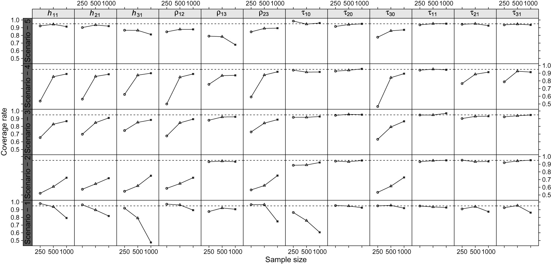
Coverage rate by scenarios and sample sizes for the heritability, correlation and dispersion parameter estimators.

The empirical coverage rate presented values close to the nominal level for scenarios 3 to 5 and large samples for all parameters. In general, for small sample sizes the coverage rate is below the nominal level. The worst results appear for the heritability index in the scenario 2. It is due to the underestimation detected in the Figure 2. Note, however, that the coverage rate for the dispersion parameters associated with the additive genetic effects is in general close to the nominal level, even for small sample sizes. It indicates that the Wald test can be used to test the null hypothesis τr1=0. In the scenario 1 the coverage rate decreases while the sample size increases. This result is compatible with the increase of the bias detected in Figures 2 and 3 and highlights the difficult to estimate when parameter values are close to the parameter space boundary.

7 Data analysis

In this section, we apply the McGLMs for mixed types of outcomes to analyse the house sparrow data set presented in Section 2. The linear predictor for each outcome was specified using the three covariates available. We adopted the identity, logit and log link functions along with constant, extended binomial and Poisson-Tweedie variance/dispersion functions for the outcomes BD, BS and AR, respectively.

The matrix linear predictor for each outcome is composed of an identity matrix combined with a relatedness matrix, representing the environmental and genetic structures respectively, see Section 3.1 for detail. The R package nadiv was employed for building the relatedness matrix based on the pedigree structure available for the house sparrow data set. As discussed in Section 3.1 we adopted the identity covariance link function.

First, we investigated the estimation of the extended binomial variance function for the outcome BS. We considered three special cases: Case 1 corresponds to the orthodox binomial variance function, i.e. p1=p2=1. Case 2 estimates p1 with the restriction p1=p2. Finally, in the case 3 both p1 and p2 are estimated. Table 1 presents estimates and standard errors for the power and dispersion parameters for each case.

The results in Table 1 show that the model in the case 3 is clearly over parametrized. Moreover, in the case 2 the estimate of the power parameter is not different of 1, i.e. the asymptotic confidence interval pˆ1±Z(1−α)/2SE(pˆ1), where Z(1−α)/2 denotes the (1−α)/2 critical value of the standard normal distribution, contains the value 1. Equivalently, the Wald test can be used as an approximation to the likelihood ratio test. For example, for choosing between the models presented as cases 1 and 2 in Table 1, the hypotheses are H0:p1=1 against H1:p1≠1 whose Z statistics is pˆ1−1/SE(pˆ1). In that case the value of the Z statistics is 1.546 which shows that the model 2 does not differ from the model 1. Thus, we choose the simplest one, i.e. model 1. Similar procedure can be used to choose between the models 1 and 3 and the results show that model 1 is the best choice for the house sparrow data set. From now on, by non-significant we means that the asymptotic confidence interval contains the value zero. The confidence level is fixed at 95%.

In all cases presented in Table 1 the dispersion parameters associated with the genetic structure (τ1) were negative, but non-significant. Table 2 presents estimates and standard errors for the joint McGLMs fitted to the house sparrow data set. The heritability index for each outcome was computed using eq. (5). To verify the effect of consider the correlation between outcomes in the fitted model, we also present estimates and standard errors obtained by fitting univariate McGLMs for each outcome.

Table 2 shows that the genetic structure has a significant effect only for the outcome BD. In that case, the heritability index is different from zero, as expected. On the other hand, for the outcomes BS and AR the heritability index was negative, but non-significant.

In general the univariate and multivariate models provide the same interpretation in terms of genetic effects. Differences appear in the size of the standard errors associated with the dispersion parameters and consequently in the standard errors of the heritability index. On average the standard errors from the joint model are 11.170% and 34.849% smaller than the ones from the univariate models, for the outcomes BS and AR, respectively. Regarding the outcome BD both models provide virtually the same estimates and standard errors.

The differences may be explained by the correlation between outcomes, whose estimates and standard errors were as follows:

The correlation between BD and BS (−0.005) and BD and AR (0.010) were non-significant. These results show that the outcomes BS and AR share no information with the outcome BD, thus the estimates from the univariate and multivariate models are virtually the same for the outcome BD. However, the correlation between BS and AR (0.8722) was significant, explaining why the standard errors from the multivariate model were smaller than the ones from the univariate models. As expected the correlation between outcomes improves the efficiency of the dispersion parameter estimators. The estimate of the power parameter suggests that the Pólya Aeppli (p=1.5) distribution is a suitable choice for the outcome AR. In order to compare the regression coefficients Figure 5 shows the regression estimates and confidence intervals obtained from the univariate and multivariate models. The intercept is not shown to avoid scale issues.

Figure 5:

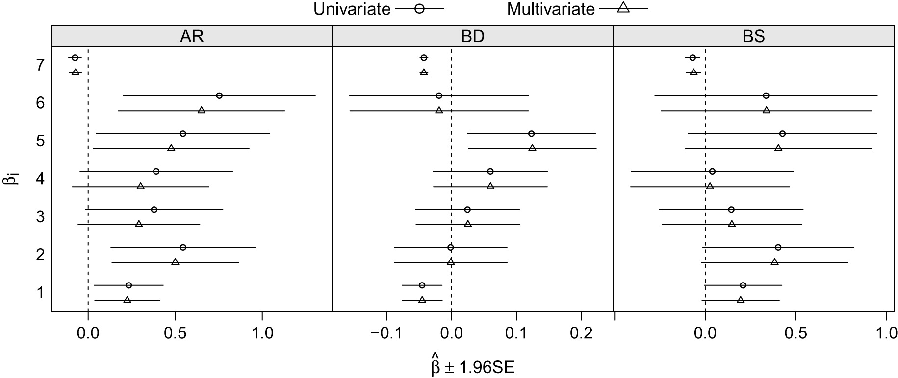
Regression parameter estimates and 95% confidence intervals by outcomes and models for the house sparrow data.

Figure 5 shows that for the outcome BD the confidence intervals from the univariate and multivariate models are really similar, in fact the difference on average is 0.015%. Regarding the outcomes AR and BS on average the confidence intervals from the multivariate model are 11.086% and 2.483% smaller than the ones from the univariate models, respectively.

[8] results showed that the heritability for BD, BS and AR were 0.35 (SE=0.07), 0.04 (SE =0.01) and 0.03 (SE =0.01), respectively. Based on the DIC values the authors concluded that the best model for the outcome BS does not include linear additive genetic effects. For the outcome AR the models without and with additive genetic effects were very close in DIC, with preference for the last one.

The results presented in Table 2 show that the heritability index for the outcome BD was 0.447 (SE =0.077). The difference between the two approaches can be due to the priory distribution requested in the context of Bayesian inference for the variance components. The priory distribution adopted by [8] was an inverse gamma, which in turn can bias downwards the heritability index. Regarding the outcomes BS and AR the estimates of the heritability are not comparable, since the models fitted in [8] were based on a conditional specification. However, the two approaches agree that for the outcome BS the additive genetic effects are not significant. Furthermore, for the outcome AR the McGLM approach shows clearly that the additive genetic effects are not significant. On the other hand, in [8] the model including the additive genetic effects shows a fit slightly better than the one without the additive genetic effects. However, as point out by [8] for small values of τ1 they observed systematic errors and priory sensitivity, mainly when using Poisson and binomial likelihood, which can explain the weak importance of the additive genetic effects, detected by their model.

8 Discussion

We presented a general statistical modelling framework for analysis of mixed types of outcomes in the context of genetic data. The models were motivated by the house sparrow data set, where a mixed of continuous, binomial and count outcomes are of interest. Furthermore, we adapted the NORTA algorithm for simulation of McGLMs and proposed a new index of heritability.

The marginal covariance structure within outcomes were modelled by means of a variance function and a matrix linear predictor combined with a covariance link function. In this paper, we focused on the identity covariance link function, since many important models used in quantitative genetic analysis appear as special cases. The variance function plays an important role in our framework, since it allows us to deal with different types of outcomes in a unified way. Furthermore, the estimation of the power parameter provides extra flexibility for our models. The linear structure of the matrix linear predictor allows us to accommodate the genetic structure as well as extend the model to deal with repeated measures, longitudinal, spatial and covariates effects. Moreover, in the context of genetic data the specification of the matrix linear predictor provides an intuitive way to define a measure of heritability for non-Gaussian data. Finally, the joint covariance matrix is specified using the generalized Kronecker product, allowing to compute the correlation between outcomes.

The second-moment assumptions allow us to adopt an estimation function approach for parameter estimation and inference. The advantages of this approach are that the estimation procedure relies on a relatively simple and efficient Newton scoring algorithm and keep the traditional population average interpretation for both regression and dispersion parameters. The simulation study presented in Section 5 showed that in general the estimating function estimators are unbiased and consistent for large samples. The simulation study also showed that for small sample size the heritability index can be strongly underestimate mainly when the parameters are close to the border of the parameter space, as appear in the scenarios 1 and 2 of our simulation study. The negative heritability index in the scenario 1 is unrealistic in terms of genetic interpretation, but in practical data analysis, such negative heritability values can appear as for example in the house sparrow data set. In general, it is associated with the non-significance of the additive genetic effects. It is also important to highlight that our estimation and inference procedure provides a Wald-type test that can be used to assess the significance of the genetic structure.

Regarding the data analysis, our results showed a significant genetic effect for the outcome BD and non-significant genetic effect for the outcomes BS and AR. These results agree with previous results obtained by [8], although these authors found a weak but still significant genetic effect for the outcome AR. The main advantages to fit a multivariate model are the possibility to compute the correlation matrix between outcomes and improve the estimation of the regression and dispersion parameters. As shown in our data analysis, in general the correlation between outcomes implies smaller standard errors for the regression and dispersion parameters.

Possible topics for further investigation and extensions include designing simulation studies to explore in detail the effect of different number of generations and families in the pedigree structure. An important aspect of the presented framework is the possibility to obtain negative heritability index. Thus, an interesting topic is to investigate from a genetic viewpoint what such negative values represent in practical data analyses. In the genetic context the genetic and environment correlations are two measures of interest. However, in the framework presented in this paper, we can assess only the correlation between outcomes (phenotypic correlation), i.e. we cannot distinguish between the genetic and environment correlations. Thus, a topic for future investigation is to propose marginal models able to distinguish between these two sources of correlation. In terms of modelling framework is interesting to investigate the performance of the McGLMs for the analysis of multivariate binary traits. Furthermore, theoretical and computational developments are required in order to construct new estimating functions to handle data not missing at random and make prediction using the Best Linear Unbiased Predictor (BLUP).

References

1. Henderson C. Estimation of genetic parameters. Ann Math Stat 1950;21:309–210.Suche in Google Scholar
2. Sorensen D, Gianola D. Likelihood, Bayesian, and MCMC methods in quantitative genetics. New York: Statistics for Biology and Health, Springer, 2007.Suche in Google Scholar
3. Dempster ER, Lerner IM. Heritability of threshold characters. Genetics 1950;35:212–236.10.1093/genetics/35.2.212Suche in Google Scholar PubMed PubMed Central
4. Hill WG. Understanding and using quantitative genetic variation. Philos Trans R Soc London, Ser B 2009;365:73–85.10.1098/rstb.2009.0203Suche in Google Scholar PubMed PubMed Central
5. Jensen H, Steinsland I, Ringsby TH, Sæther B-E. Evolutionary dynamics of a sexual ornament in the house sparrow (Passer domesticus): the role of indirect selection within and beween sexes. Evolution 2008;62:1275–1293.10.1111/j.1558-5646.2008.00395.xSuche in Google Scholar PubMed
6. Gianola D, Fernando RL. Bayesian methods in animal breeding theory. J Anim Sci 1986;63:217–244.10.2527/jas1986.631217xSuche in Google Scholar
7. Hadfield JD, Nakagawa S. General quantitative genetic methods for comparative biology: phylogenies, taxonomies and multi-trait models for continuous and categorical characters. J Evol Biol 2010;23:494–508.10.1111/j.1420-9101.2009.01915.xSuche in Google Scholar PubMed
8. Holand AM, Steinsland I, Martino S, Jensen H. Animal models and integrated nested Laplace approximations. G3: Genes, Genome, Genetics, 2013;3:1241–1251.10.1534/g3.113.006700Suche in Google Scholar PubMed PubMed Central
9. McCulloch CE. Maximum likelihood algorithms for generalized linear mixed models. J Am Stat Assoc 1997;92:162–170.10.1080/01621459.1997.10473613Suche in Google Scholar
10. Fong Y, Rue H, Wakefield J. Bayesian inference for generalized linear mixed models. Biostatistics 2010;11:397–412.10.1093/biostatistics/kxp053Suche in Google Scholar PubMed PubMed Central
11. Hadfield JD. MCMC methods for multi-response generalized linear mixed models: the MCMCglmm R package. J Stat Software 2010;33:1–22.10.18637/jss.v033.i02Suche in Google Scholar
12. Rue H, Martino S, Chopin N. Approximate Bayesian inference for latent Gaussian models by using integrated nested Laplace approximations. J R Stat Soc, Ser B 2009;71:319–392.10.1111/j.1467-9868.2008.00700.xSuche in Google Scholar
13. Liu J, Huang J, Ma S. Penalized multivariate linear mixed model for longitudinal genome-wide association studies. BMC Proc 2014;8:1–4.10.1186/1753-6561-8-S1-S73Suche in Google Scholar
14. Liu J, Yang C, Shi X, Li C, Huang J, Zhao H, Ma S. Analyzing association mapping in pedigree-based gwas using a penalized multitrait mixed model. Genet Epidemiol 2016;40:382–393.10.1002/gepi.21975Suche in Google Scholar PubMed
15. de Villemereuil P, Schielzeth H, Nakagawa S, Morrissey M. General methods for evolutionary quantitative genetic inference from generalised mixed models. Genetics 2016;204(3):1281–1294.10.1534/genetics.115.186536Suche in Google Scholar
16. Bonat WH, Jørgensen B. Multivariate covariance generalized linear models. J R Stat Soc, Ser C 2016;65:649–675.10.1111/rssc.12145Suche in Google Scholar
17. Liang K-Y, Zeger SL. Longitudinal data analysis using generalized linear models. Biometrika 1986;73:13–22.10.1093/biomet/73.1.13Suche in Google Scholar
18. Carey VJ. gee: generalized estimation equation solver, 2015, http://CRAN.R-project.org/package=gee, r package version 4.13-19.Suche in Google Scholar
19. Højsgaard S, Halekoh U, The Yan J. R package geepack for generalized estimating equations. J Stat Software 2006;15:1–11.10.18637/jss.v015.i02Suche in Google Scholar
20. Jørgensen B, Knudsen SJ. Parameter orthogonality and bias adjustment for estimating functions. Scand J Stat 2004;31, 93–114.10.1111/j.1467-9469.2004.00375.xSuche in Google Scholar
21. Hall DB, Severini TA. Extended generalized estimating equations for clustered data. J Am Stat Assoc 1998;93, 1365–1375.10.1080/01621459.1998.10473798Suche in Google Scholar
22. Diggle PJ, Heagerty P, Liang K-Y, Zeger SL. Analysis of longitudinal data. Oxford: Oxford Statistical Science Series, 2002.Suche in Google Scholar
23. Cario MC, Nelson BL. Modeling and generating random vectors with arbitrary marginal distributions and correlation matrix, Technical report, Northwestern University, 1997.Suche in Google Scholar
24. Core Team R. Language R: A and Environment for Statistical Computing, R Foundation for Statistical Computing, Vienna, Austria, 2015, ISBN 3-900051-07-0.Suche in Google Scholar
25. Pärn H, Jensen H, Ringsby TH, Sæther B-E. Sex-specific fitness correlates of dispersal in a house sparrow metapopulation. J An Ecol 2009;78:1216–1225.10.1111/j.1365-2656.2009.01597.xSuche in Google Scholar
26. Ringsby TH, B-E Sæther, Tufto J, Jensen H, Solberg EJ. Asynchronous spatiotemporal demography of a house sparrow metapopulation in a correlated environment. Ecology 2002;83:561–569.10.1890/0012-9658(2002)083[0561:ASDOAH]2.0.CO;2Suche in Google Scholar
27. Martinez-Beneito MA. A general modelling framework for multivariate disease mapping. Biometrika 2013;100:539–553.10.1093/biomet/ast023Suche in Google Scholar
28. Bonat WH, Kokonendji CC. Flexible Tweedie regression models for continuous data. J Stat Comput Simul 2017;87:2138–2152.10.1080/00949655.2017.1318876Suche in Google Scholar
29. Jø rgensen B. Exponential dispersion models. J R Stat Soc, Ser B 1987:49:127–162.10.1111/j.2517-6161.1987.tb01685.xSuche in Google Scholar
30. Jø rgensen B. The theory of dispersion models. London: Chapman & Hall, 1997.Suche in Google Scholar
31. Barndorff-Nielsen O, Jø rgensen B. Some parametric models on the simplex. J Multivariate Anal, 1991;39:106–116.10.1016/0047-259X(91)90008-PSuche in Google Scholar
32. Bonat WH, Olivero J, Grande-Verga M, Fárfan MA, Fa JE. Modelling the covariance structure in marginal multivariate count models. J Agric Biol Environ Stat 2017;1–19.Suche in Google Scholar
33. Jø rgensen B, Kokonendji C. Discrete dispersion models and their Tweedie asymptotics. AStA Adv Stat Anal 2015;100:43–78.10.1007/s10182-015-0250-zSuche in Google Scholar
34. Bonat WH. mcglm: multivariate covariance generalized linear models, 2016. http://git.leg.ufpr.br/wbonat/mcglm, R package version 0.3.0.Suche in Google Scholar
35. Anderson TW. Asymptotically efficient estimation of covariance matrices with linear structure. The Ann Stat 1973;1:135–141.10.1214/aos/1193342389Suche in Google Scholar
36. Pourahmadi M. Maximum likelihood estimation of generalised linear models for multivariate normal covariance matrix. Biometrika 2000;87:425–435.10.1093/biomet/87.2.425Suche in Google Scholar
37. Lynch M, Walsh B. Genetics and analysis of quantitative traits. Oxford: Sinauer, 1998.Suche in Google Scholar
38. Demidenko E. Mixed models: theory and applications with R. New Jersey: Wiley, 2013.Suche in Google Scholar
39. Wolak ME. nadiv: an R package to create relatedness matrices for estimating non-additive genetic variances in animal models. Meth Ecol Evol 2012;3:792–796.10.1111/j.2041-210X.2012.00213.xSuche in Google Scholar
40. Self SG, Liang K-Y. Asymptotic properties of maximum likelihood estimators and likelihood ratio tests under nonstandard conditions. J Am Stat Assoc 1987;82:605–610.10.1080/01621459.1987.10478472Suche in Google Scholar
41. Crainiceanu CM, Ruppert D. Likelihood ratio tests in linear mixed models with one variance component. J R Stat Soc, Ser B 2004;66:165–185.10.1111/j.1467-9868.2004.00438.xSuche in Google Scholar
42. Stram DO, Lee JW. Variance components testing in the longitudinal mixed effects model. Biometrics 1994;50:1171–1177.10.2307/2533455Suche in Google Scholar PubMed
43. Huifen C. Initialization for norta: generation of random vectors with specified marginals and correlations. INFORMS J Comput 2001;13:312–331.10.1287/ijoc.13.4.312.9736Suche in Google Scholar
44. NORTARA: Su P. generation of multivariate data with arbitrary marginals, 2014, R package version 1.0.0.Suche in Google Scholar
45. Coster A. pedigree: pedigree functions, 2013, R package version 1.4.Suche in Google Scholar
Supplemental Material
The R code and data set are available in the supplementary material website.http://www.leg.ufpr.br/doku.php/publications:papercompanions:biometrics
© 2017 Walter de Gruyter GmbH, Berlin/Boston
Artikel in diesem Heft
- Estimation and Inference for the Mediation Proportion
- Adaptation of Chain Event Graphs for use with Case-Control Studies in Epidemiology