Multi-locus Test and Correction for Confounding Effects in Genome-Wide Association Studies

1 Introduction

Genome-wide association studies (GWAS) contain a large number of genetic variants, i. e., single nucleotide polymorphisms (SNP), for hundreds or thousands of subjects. SNPs are single base differences in DNA sequences among individuals and can serve as genetic markers for identifying disease susceptibility genes. A SNP has three possible genotypes, wild type homozygous, heterozygous, and mutation homozygous. In a GWAS, genotypes of up to millions of SNPs are measured for disease (case) and normal (control) subjects, where differences in SNP genotype frequency between cases and controls imply genetic associations with the disease.

In most situations, statistical analysis of genome-wide association data has been on a single SNP at a time, using simple logistic regression or χ2 tests of association [1]. However, with the large number of SNP variables, these methods may produce too many significant results, majority of which are false positives. Recently, multi-locus or multi-SNP association tests have been proposed to improve single SNP analysis [2–4], aiming at detecting combinatorial effects of multiple SNPs. Our work follows this line. We consider a block of 5–15 SNPs and scan the whole genome with SNP blocks for disease association.

Another challenge of GWAS data analysis is the presence of confounding effects. Jakobsdottir et al. [5] examined the viability of using significant SNPs from GWASs as biomarkers for predicting the risk of several diseases, for example, macular degeneration, type II diabetes, Crohn’s disease, and cardiovascular disease. It was found that the predictive power of the significant SNPs was generally poor and using SNPs could not perform better than the commonly known standards for predicting the diseases. Although GWASs tried to follow a randomized case-control design, there are a substantial amount of potential confounding factors in the data and there is often no clear choice of what the control sample should be. Some examples of confounding factors particular to GWASs are 1) genetic artifacts, i. e., systematic “errors” on the SNP array chips, 2) phenotypical and environmental heterogeneity of the subjects such as gender, ancestry, age, etc., and 3) ignorance of disease pathobiology [6–8]. Most confounding factors in GWASs are difficult to quantify as they are not directly observable.

For known confounding factors, e. g., gender, age, known disease conditions etc., multivariate logistic regression is commonly used for disease association of a SNP conditional on the confounding factors. For complicated confounding factors, e. g., latent population structure, Devlin and Roeder [9] developed a method, called Genomic Control, to measure the extent of inflation due to population stratification. Price et al. [10] used principal components analysis to identify principal components of ancestry that may demonstrate population structures. An extensive review of methods that correct for population stratification are in Price et al. [11]. A limitation of these methods is that they mainly work for population stratification but may not account for other types of confounding effects.

In this paper we propose a weighted χ2 test for big contingency table from a block of multiple SNPs and develop statistical methods that identify and eliminate confounding effects. Our basic idea is to study genotype frequencies of a block of SNPs conditional on all other SNPs, which are not associated with the disease of interest. More specifically, we define a latent confounding factor, named balancing score, using profile of the genome-wide SNPs, then we apply sample matching or stratification via the balancing score to eliminate confounding effects.

We demonstrate our methods on a simulated GWAS and a GWAS of rheumatoid arthritis, which is the GAW16 (Genetic Analysis Workshop 16) data from the North American Rheumatoid Arthritis Consortium. We compare the proposed methods with an existing multi-SNP approach, called Sequence Kernel Association Test (SKAT, Wu et al. [2]), and methods that correct for population stratification, including Genomic Control (Devlin and Roeder [9]) and principal components analysis (EIGENSTRAT, Price et al. [10]). The comparisons show that the proposed method based on the balancing score dramatically removes the number of significant tests, or false positives, and performs superior to the existing methods.

The rest of the paper is organized as follows. In Section 2, we propose a test for a big contingency table when we assess disease association of a block of SNPs. Section 3 introduces the rheumatoid arthritis GWAS and shows the phenomenon of false positive significances. In Section 4, we develop the method of balancing score, to identify confounding effects embedded in GWASs. In Section 5, we conduct simulation studies to compare our methods with SKAT, Genomic Control and EIGENSTRAT. We apply our method in the rheumatoid arthritis GWAS in Section 6. Finally, we conclude with a discussion in Section 7.

2 Large scale contingency tables for multiple SNPs

In GWAS data analysis, we scan the whole genome and compare disease subjects with normal subjects in terms of genotype frequencies. Significant difference of genotype frequencies at a genomic region implies association with the disease. The commonly used statistical methods analyze SNPs one at a time. We, however, consider a block of consecutive SNPs and analyze combinatorial effects of the SNP block. We use SNP blocks to scan the whole genome and hence refer to blocks as moving windows. For any given window of δ SNPs there are 3δ possible genotypes. If we use a window of size 10, it results in up to 310=59,049 different genotypes. In practice, due to the limit in sample size, which is typically a few thousands, no more than 1,000 genotypes tend to be observed. For each window, tabulating the number of case and control subjects for each genotype results in a 2×K contingency table, where K represents the number of genotypes present in the sample for this particular window. For a window of size 10, K is typically hundreds but many cells have very small counts.

There are different ways to model the count data in a 2×K contingency table. Here we choose to start with a Poisson model, which has been used by Liu and Xie [12] in another work of SNP data analysis. This model is effectively equivalent to a multinomial model for inference of the SNP count data. Let Nj(i) denote a Poisson count with unknown rates λj(i)≥0 for i=0,1 and j=1,…,K. The count Nj(0) represents the number of subjects (or occurrences) of genotype j in the control group and Nj(1) is the number of subjects (occurrences) of genotype j in the disease group. They are modeled as two independent Poisson counts with the respective rates λj(0) and λj(1). The rates λj(0) and λj(1) are the expected numbers of occurrences of genotype j in the corresponding populations. Denote the row total of the contingency table as mi=∑j=1KNj(i) for i=0 and 1, then conditioning on mi the observed counts Nj(i), j=1,…,K, follow a multinomial distribution

where θj(i)=λj(i)/∑l=1Kλl(i).

For a given window, there are two independent multinomial distributions for SNP genotypes of the control and case populations. We are interested in testing a null hypothesis

which corresponds to no difference between the case and control populations for the given SNP window, or the SNP window is not associated with the disease. This hypothesis is equivalent to λj(0)=cλj(1) for all j=1,…,K based on the original Poisson counts model, where c is a constant. An alternative parametrization is to consider the Poisson counts conditioning on each column total of the 2×K table, which yields K independent binomial distributions. More specifically, let ϕj=λj(1)/(λj(1)+λj(0)) and denote nj=Nj(0)+Nj(1) and Xj=Nj(1) for j=1,…,K. We have

The null hypothesis (1) is equivalent to

Our test for a disease associated SNP window is based on this hypothesis. Let us denote N=∑j=1Knj, which is the total sample size of both control and case groups. We introduce a test statistic:

where ϕˆ0=(∑j=1KXj)/N is an estimate of the common binomial frequency under H0 and wj=(nj−1)/(nj+1) down-weights counts with small column total of nj. The weights such defined exclude columns whose total is 1 but do not affect columns with a large number of counts. We approximate the distribution of Y under the null hypothesis by a scaled χ2 distribution, where the scale and degrees of freedom are obtained by approximating each term in the sum, e. g., Xj, by a normal distribution and calculating the first and second moments of the statistic accordingly. The validity of the null distribution is demonstrated by data permutation as described in the next section. We calculate the test statistic (2) for every SNP window and claim significance if its p-value from the scaled χ2 distribution is smaller than a p-value cutoff, e. g., 0.0001.

3 False positive significance

We have applied the weighted χ2 tests on the GAW16 (Genetic Analysis Workshop 16) data from the North American Rheumatoid Arthritis Consortium. This GWAS aims at identifying genetic variants, more specifically SNPs, which are associated with the rheumatoid arthritis disease. The data consists of 2,062 samples, where 868 are cases and 1,194 are controls. For each sample, whole genome SNPs are observed with a coverage of 545,080 SNPs. We prune the GWAS data to remove SNPs that have 1) the Hardy-Weinberg p-values ≤0.0001; 2) genotype missing rates >0.05; 3) minor allele frequencies <0.001. There are 513,942 SNPs after the filtering. For sample filtering, no individual is removed with a missing genotype rate>0.07.

We first examine the test statistic Y, as defined in (2), and its null distribution by running the test on permuted data of the rheumatoid arthritis GWAS. All of the 2,062 subjects in the study are randomly assigned into the case and control groups ignoring their true disease statuses, whereas the correlation structure of the SNP genotypes has not been disturbed. The permutation thus generates two groups of samples that have no difference in genotype distributions but keep the same SNP correlation structure as the original data. We then scan the whole genome by a SNP window of size 10 and compute Y for all SNP windows. The quantile-to-quantile (QQ) plots of Y are exactly straight lines for all chromosomes (plots not shown), indicating that the weighted χ2 distribution of Y describes the null distribution well.

However, when we apply the test statistic Y (2) to the real data, there are a great amount of significances for any chromosomes. This is indicated by the large observed z-values in the QQ-plots for all chromosomes, on tails of the QQ-plots on the first panel in Figure 7, where z-values are calculated as Z=Φ−1(F(Y)) with F(⋅) being the proposed scaled χ2 distribution for Y and Φ(⋅) being the standard normal distribution. For the rheumatoid arthritis disease, only the HLA (human leukocyte antigen) region in Chromosome 6 has been replicated in multiple association studies and has consistent evidence of contributing to disease risk. We believe that majority of the significant test statistics on the other chromosomes are false positives. In the next section we develop a method that identifies confounding effects and provides improved statistical analysis in the GWAS.

4 Balancing score

Noticing that the false positives are located almost everywhere among all chromosomes, we find it sensible to believe that the case and the control samples are not matched well, at least, not balanced on genotypes that are not associated with the disease. This is a fundamental problem in disease studies. In general, even with case and control samples that have been well balanced on observed phenotypes, there is still a need to balance on genotypes that are not related to the disease of interest. We take a good use of genetic information and consider that unknown confounding factors are embedded in the profile of genome-wide SNPs.

Let SU denote the indices of the SNPs that are not associated with the disease and SD denote the SNPs that are associated with the disease. When we study a given SNP block and calculate the test statistic Y (2), ideally the case and control samples should be balanced on the genotypes that are not associated with the disease, i. e., SU. To account for unbalanced samples, or confounding effects, we can calculate the test statistic Y conditional on SU or create matched case and control samples according to SU. However, we do not know which SNPs are SU and which are SD. In other words, SNPs that can be used for capturing confounding effects are mixed with those associated the disease. We assume that majority of the SNPs are not associated with the disease hence the whole sequence will be utilized to define a balancing score for confounding factors.

We use the previous notations in large contingency tables, i. e., θ1(1),…,θK(1) denote the frequencies of all possible genotypes of a given SNP window in the case group and θ1(0),…,θK(0) denote the frequencies of the genotypes in the control group. We also introduce additional indices,

i−agivensubject,

k0−agivenSNPwindowunderstudy,

k−allotherSNPwindows,gik−genotypeofsubjectiatSNPwindowk.

Note that gik is a combinatorial genotype of multiple SNPs, e.g, 10 SNPs, and has K categories. Let

We define a balancing score for subject i as pi=∑k≠k0pik/∑k≠k01, averaging over all SNP windows in the genome except the SNPs under study. Due to the large number of SNP windows from the whole genome, whether or not including the current SNP window k0 in the calculation does not change the value of the balancing score for subject i. For simplicity we use all SNP windows in the calculation. Sample frequencies θˆ1(1),…,θˆK(1) and θˆ1(0),…,θˆK(0) are used in calculating pik, where θˆj, j=1,…,K, is the count of genotype j divided by the sample size, in the case or control group respectively. We exclude the current subject i in calculating the sample frequencies. The balancing score is a likelihood ratio from the whole-genome information. We show next that it is able to identify confounding effects, which may come from population structures as well as other unknown confounding factors.

Figure 1:

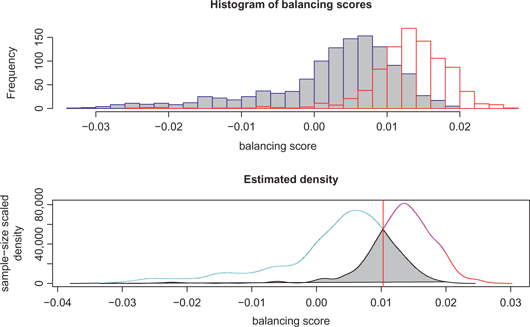
Histograms of the balancing scores (in the logarithm scale) for the case and control samples, where cases are represented in red on the right hand side and controls are represented in blue on the left hand side.

We calculate the balancing scores for all 2,062 subjects in the rheumatoid arthritis GWAS. Figure 1 shows histograms of the balancing scores, in the logarithm scale, from subjects in the case group (red color and on the right hand side) and subjects in the control group (blue color and on the left hand side) respectively. The figures indicate that there are apparent differences between the case and the control groups. In other words, the case and the control groups do not have a balanced distribution in terms of the balancing score. We conclude that confounding effects exist in this rheumatoid arthritis GWAS. In general, less overlap between the case and the control distributions, stronger confounding effects. On the contrary, more overlap between the case and the control distributions, less confounding effects are identified. In Section 6, we will show the latter is the case in the principal components analysis of this data set.

We can interpret the balancing score as a summary feature of all possible confounding factors for the respective subject, where the confounding factors are not limited to population stratification. The confounding effects need to be controlled when we compare the case and the control samples. A simple approach is the sample matching method, which matches a case subject to a control subject with respect to their balancing scores. Without loss of generality, assume control subjects tend to have lower balancing scores. We define a cutoff line at the intersection of the two density curves of the balancing scores for the case and control subjects, as shown by the vertical line in Figure 1. To the left of the cutoff line, where there are more control samples than the cases, every case is matched to a control subject with the nearest balancing score. That is, the control subject most similar to a given case in terms of balancing score is selected for a case-control matching pair. In a rare situation that two control samples have exactly the same balancing score with the case, one control is arbitrarily selected. Analogously, to the right of the cutoff line, where there are more case samples than the controls, every control sample matches a case with the nearest balancing score. This procedure matches subjects only in the intersection of the two balancing score distributions and subjects cannot be matched twice. The weighted χ2 test statistic previously defined will then be applied in the matched samples and calculated along the genome for significant SNP blocks.

The balancing score can also be used in a stratified analysis. We place subjects into B strata according to their balancing scores. The proposed test statistic Y (2) can be calculated within each stratum and recombined. Denote Yb as the test statistic in stratum b, and nb is the number of subjects in the stratum, b=1,…,B. We define a stratified test statistic

Each Yb will still be a scaled χ2 distribution but because each Yb is weighted by nb/N the test statistic Ystrata will no longer follow a χ2 distribution. We use an approximation for distribution function of a linear combination of χ2 test statistics by Moschopoulos and Canada [13] to estimate the null distribution of Ystrata. The approach estimates the distribution function of Ystrata by first expressing the moment generating function of Ystrata as an infinite sum of gamma densities. The distribution function is then calculated upon inversion. Although the estimation was originally intended for χ2 distributions of small degrees of freedom, our simulations demonstrate that this approach also works well for linear combinations of χ2 distributions with degrees of freedom as large as two hundred.

5 Simulation studies

The simulation is similar to those in Price et al. [10], where confounding effects are simply from population stratification. We demonstrate that the proposed method works very well, although the simulation scenario is in favor of the principal components analysis method.

We generate genotype data of 100,000 SNPs for 500 cases and 500 controls. We consider a mixture of two populations in the samples. For the 500 cases, a proportion q of the samples are from population 1 and 1−q from population 2. For the 500 controls, a proportion r of the samples are from population 1 and 1−r from population 2. We consider two scenarios: 1) q=r, for example, both are 50 %, which corresponds to no population stratification; 2) q≠r, for example, q=60% and r=40%, which gives population stratification. When there is population stratification, there are three types of SNPs along the sequence of 100,000 SNPs: causal SNPs, random SNPs with no association with disease, and differentiated SNPs with no association. Causal SNPs are in positions 5000, 5002, 5004, 5006, 5008, and 10000, 10002, 10004, 10006, 10008. SNPs in all other positions are either random SNPs (70 %) or differentiated SNPs (30 %). For a random SNP, allele frequencies for population 1 and population 2 are generated using the Balding-Nichols model [14] with FST=0.01, where FST=0.01 is defined in Price et al. [10] as a parameter to specify allele frequency differences for typical common SNPs. For a differentiated SNP, we assume population allele frequencies of 0.80 for population 1 and 0.20 for population 2. The differentiated SNPs have no association with disease but different allele frequencies due to population stratification. For a causal SNP, we use the Balding-Nichols model with FST=0.01 and a multiplicative disease risk model with a relative risk of 3 for the causal allele.

We generate ten simulation data sets for both scenarios of no population stratification and population substructure. We then compare a variety of association tests under each scenario in Table 1. The association tests include the standard Armitage trend χ2 test [15] for single SNPs one by one, EIGENSTRAT [10] that uses principal components to correct for population confounding effects, SKAT [2] that examines multiple SNPs but does not consider confounding effects (only for the case of no population stratification), SKAT adjusting for the first two principal components (PCs) of population substructure (only for the case of population stratification), the weighted χ2 test Y as in (2) without sample matching, and our weighted χ2 test based on balancing score matching samples. We use a block of five SNPs for SKAT and our methods. That is, the SNP window is of size 5. For all methods, the corresponding association statistics producing a p-value < 0.0001 are reported as significance. There are two situations for significant results: 1) those among the causal SNPs or SNP windows, which are true positives; 2) those among the non-causal SNPs or SNP windows, which are false positives. The association test that identifies the largest number of true positives and the appropriate number of false positives, around 0.0001×100,000=10 for the p-value cutoff of 0.0001, is an optimal one.

Table 1 shows the average numbers of significant SNPs or SNP windows by different methods in ten simulations. Note that the Armitage and EIGENSTRAT tests are for SNPs one by one, but SKAT and our method test for multiple SNPs. There are 10 causal SNPs but 18 causal SNP windows, where a causal window is referred to as a window of size 5 that contains at least two causal SNPs. For the scenario of no population stratification, the standard SKAT is used, which does not account for confounding effects. For the scenario of population stratification, we include the first two principal components of the genotype data in the SKAT regression model, so that it also corrects for the population substructure. Our simulations indicate that when there is no population confounding effect, all methods work well. However, when there is population stratification, the methods that do not consider confounding effect, i. e., Armitage and unmatched Y, detect too many false positives. Our proposed weighted χ2 test based on balancing score matching samples attains an appropriate type I error (0.0001×100,000=10) and achieves superior power for true associations (17.7 out 18), whereas SKAT after adjusting for population principal components gives fewer true positives (14.4 out of 18) and slightly larger false positives. EIGENSTRAT is also able to correct the confounding effect of population structure, as expected for this simulation study.

Figure 2:

QQ-plots of four methods of association tests for the simulation data.

Figure 2 shows QQ-plots of four associate tests for one simulation. Besides Armitage, EIGENSTRAT, and our balancing score method, we also illustrate the Genomic Control adjusted test, which divides the Armitage test by the Genomic Control factor λ [9]. The standard Armitage χ2 test gives inflated associations. The Genomic Control factor λ=9.422 indicates strong population stratification. However, the Genomic Control adjusted association test does not identify any significant SNPs, as no tail shows up in its QQ-plot. On the other hand, both EIGENSTRAT and our method are able to detect associations after correcting for population confounding effects.

6 Application in a GWAS

We have applied the Armitage χ2 test, Genomic Control, SKAT, EIGENSTRAT and our method in the GWAS data of rheumatoid arthritis. The Genomic Control factor of the GWAS data is λ=1.4701, demonstrating existence of confounding effects. Our method considers multiple SNPs and corrects for confounding effects. We first plot the autocorrelation of the Armitage statistics one by one chromosome, to evaluate how many SNPs are correlated for window size selection. The autocorrelation plots of the first four chromosomes are shown in Figure 3. The big reduction of the autocorrelation around lag 10 indicates that a window size 10 is a fine choice. We further examine the effect of window size by implementing our proposed method with diverse window sizes, 2, 5, 10 and 15, respectively. More specifically, we study how different window sizes affect the number of significances (p-values ≤10−6). Figure 4 illustrates the number of significances over different window sizes for several chromosomes as typical examples. For most chromosomes, the number of significances is very small and do not vary with different window sizes, as represented by the lines of Chromosome 2. But for Chromosome 3, 6, 9, and 10, the number of significances gradually increase along window sizes (Chromosome 6 is not shown in the figure due to the known large number of significances). Based on these analyses, we decide to use the window size 10.

Figure 3:

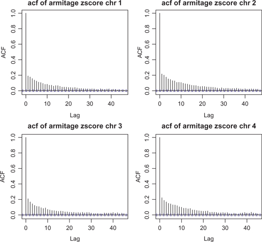
The autocorrelation function (acf) of the Armitage statistic for the first four chromosomes of the GWAS data of rheumatoid arthritis. The reduction of SNP autocorrelation over lag values indicates that the SNP window size 10 is a fine choice.

Figure 4:

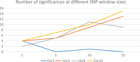
Effect of SNP window size as indicated by the number of significances over different window sizes. Most chromosomes are similar to the lines of Chromosome 2 at the bottom, with very few significances.

Applying our method, we have previously showed that there is substantial difference in the distributions of the balancing scores between the case subjects and the control subjects (Figure 1). Hence, our method correctly identifies the confounding effect. On the other hand, Figure 5 demonstrates that the first two principal components from EIGENSTRAT have great overlaps between the distributions of the case subjects and the control subjects. As the distributions are similar between the case and control groups, the principal components from EIGENSTRAT do not find the confounding effects that are indicated by the balancing score.

Figure 5:

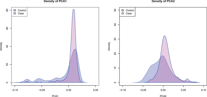
Distributions of the top two principal components from EIGENSTRAT in the case and control groups. The great overlaps indicate the principal components analysis is not able to identify the confounding effect in the GWAS data set.

Figure 6:

QQ-plots of five methods of association tests for Chromosome 1 in the rheumatoid arthritis GWAS. Tails on the top of the plots are likely false positives.

Figure 6 displays QQ-plots of five association tests for Chromosome 1, which comprises 40,929 SNPs. We use p-value<0.0001 as a threshold for significance here. Under the assumption that Chromosome 1 has no true SNP association, we expect 4 significances out of 40,929 SNPs, purely due to Type I errors. The Armitage χ2 test gives 174 significances, Genomic Control and EIGENSTRAT give 18 and 17 significances respectively, and our method gives 4. These results suggest that it is very likely that Chromosome 1 does not contain any causal SNP and our method is able to produce the correct number of significances. Genomic Control and EIGENSTRAT correct confounding effects to a certain level but seem to still produce spurious associations. Indeed, the Genomic Control factor of EIGENSTRAT is λ=1.06 for the whole genome, implying moderate confounding effects after the correction. On the other hand, the Genomic Control factor of our method is λ=0.87, showing no confounding effects any more after the correction. In fact, the p-values of our method are slightly skewed toward 1.

The QQ-plots of our method for all chromosomes are shown on the second panel in Figure 7. The number of significant test statistics is greatly reduced for all chromosomes except for Chromosome 6. The excessive number of false positives on the first panel in Figure 7 are removed by adjusting for the balancing score. The significant SNP windows in Chromosome 6 correspond to the known disease associated gene HLA. Most other chromosomes do not have any significant SNP windows. The significant SNP windows in Chromosome 3, 9, 10, and 22 suggest possible genetic variants that may associate with the disease rheumatoid arthritis.

Figure 7:

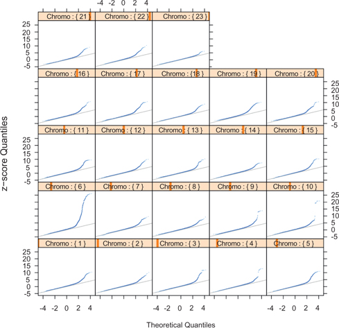
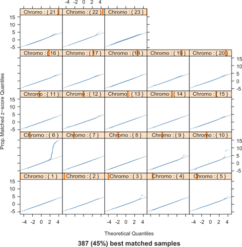
Comparison of the amount of false significant test statistics (the up tails of the QQ plots) for the raw data (the first panel) and the balancing score matched data (the second panel). The first panel: QQ-plots of the proposed test statistic Y for SNP blocks in each chromosome from the GWAS of rheumatoid arthritis. The test statistic is converted to a z-score, Z=Φ−1(F(Y)), where F(⋅) is the proposed scaled χ2 distribution for Y. The second panel: QQ-plots of the test statistic Y but for matched samples.

To study the issue of automatic reduction of false positives due to the smaller sample size of about 400 matched pairs, we calculate the proposed test statistic Y for 387 unmatched pairs, with 387 random case and 387 random control subjects. We find that although the number of false positives does decrease it is still greater than what would be expected in multiple comparisons when assuming all null hypotheses are true. This shows not only that the balancing score is able to produce a more balanced sample set but also that confounding can be very prevalent in even small sample sizes.

Alternatively, we stratify all 2,062 subjects in the rheumatoid arthritis GWAS into B=3 or 5 strata by their balancing scores. The test statistic Ystrata is calculated for all SNP windows, each of size 10. For either 3 or 5 strata, the QQ-plots are very similar to the second panel of Figure 7, sufficiently removing a large portion of false positives. The most significant SNP windows are also consistent with the results of the matching method. We conclude that our analysis controls underlying confounding factors and hence provides more accurate significance test results than the standard methods.

7 Discussion

We define a balancing score that represents potential confounding factors from the genome-wide SNP profile. Different distributions of the balancing scores between the case and the control groups indicate confounding effects. We propose the matching and stratification methods that emulate a more balanced design prior to analysis. Our methods are specially useful when confounding factors are unknown and not limited to population stratification. Although the balancing score is particularly defined for blocks of multiple SNPs, it can also be calculated for single-SNP analysis. In fact, we may simply consider a SNP window size 1 with three genotypes of the single SNP. The calculation as in Section 4 follows automatically.

A slight and known tradeoff to the matching approach is the possible reduction of sensitivity due to the loss of subjects in the analysis. We argue however that the removal of confounding effects greatly outweighs the loss in sensitivity, especially as we were able to still declare significance of the association between SNPs in Chromosome 6 and the prevalence of rheumatoid arthritis in the given GWAS.

Although we recommend our technique for any GWAS study, it is not the end-all-be-all solution to controlling confounding effects. Because the balancing score is a summarized measure it may not be able to adjust for some specific confounding factors as the effect can be “lost” within the summarization. Thus we recommend our technique be used not as a substitute for current methods that adjust GWAS studies for known confounding variables but rather as a technique to augment analysis. If a known confounding factor affects analysis, it may be prudent to adjust analysis prior to estimating the balancing score. For example if gender is known to alter the likelihood of a subject being affected by disease we suggest stratifying subjects by gender and then calculating the balancing score within each stratum. Adjusting for a known confounding variable will likely trump the effect of the balancing score but the advantage of the balancing score is more specifically to adjust for unknown confounding variables which can potentially exist in any study. As such our method may be seen as an exploratory method as well to identify the degree of confound effects among the subjects. Additionally, this technique is not limited to GWAS studies but can be employed for any case-control study involving genomic sequence data.

References

1. McCarthy M, Abecasis G, Cardon L, Goldstein D, Little J, Ioannidis J, et al. Genome-wide association studies for complex traits: consensus, uncertainty and challenges. Nat Rev Genet 2008;9(5):356–69.10.1038/nrg2344Suche in Google Scholar PubMed
2. Wu MC, Lee S, Cai T, Li Y, Boehnke M, Lin X. Rare-variant association testing for sequencing data with the sequence Kernel association test. Am J Human Genet 2011;89:82–93.10.1016/j.ajhg.2011.05.029Suche in Google Scholar PubMed PubMed Central
3. Zhang Y. A novel bayesian graphical model for genome-wide multi-snp association mapping. Genet Epidemiol 2012;36:36–47.10.1002/gepi.20661Suche in Google Scholar PubMed PubMed Central
4. Qiao D, Cho MH, Fier H, Bakke PS, Gulsvik A, Silverman EK, et al. On the simultaneous association analysis of large genomic regions: a massive multi-locus association test. Bioinformatics 2014;30:157–64.10.1093/bioinformatics/btt654Suche in Google Scholar PubMed PubMed Central
5. Jakobsdottir J, Gorin MB, Conley YP, Ferrell RE, Weeks DE. Interpretation of genetic association studies: Markers with replicated highly significant odds ratios may be poor classifiers. PLoS Genet 2009;5:e10000337.10.1371/journal.pgen.1000337Suche in Google Scholar PubMed PubMed Central
6. Begum F, Ghosh D, Tseng GC, Feingold E. Comprehensive literature review and statistical considerations for gwas meta-analysis. Nucleic Acids Res 2012;40:3777–84.10.1093/nar/gkr1255Suche in Google Scholar PubMed PubMed Central
7. Moore JH, Asselbergs FW, Williams SM. Bioinformatics challenges for genome-wide association studies. Bioinformatics 2010;26:445–55.10.1093/bioinformatics/btp713Suche in Google Scholar PubMed PubMed Central
8. Tian C, Gregersen PK, Seldin MF. Accounting for ancestry: population substructure and genome-wide association studies. Human Mol Genet 2008;17:R143–R150.10.1093/hmg/ddn268Suche in Google Scholar PubMed PubMed Central
9. Devlin B, Roeder K. Genomic control for association studies. Biometrics 1999;55(4):997–1004.10.1111/j.0006-341X.1999.00997.xSuche in Google Scholar
10. Price AL, Patterson NJ, Plenge RM, Weinblatt ME, Shadick NA, Reich D. Principal components analysis corrects for stratification in genome-wide association studies. Nat Genet 2006;38:904–9.10.1038/ng1847Suche in Google Scholar PubMed
11. Price AL, Zaitlen NA, Reich D, Patterson N. New approaches to population stratification in genome-wide association studies. Nat Rev Genet 2010;11:459–63.10.1038/nrg2813Suche in Google Scholar
12. Liu C, Xie J. Large scale two sample multinomial inferences and its applications in genome wide association studies. Int J Approximate Reasoning 2013. doi:10.1016/j.ijar.2013.04.010Suche in Google Scholar
13. Moschopoulos P, Canada WB. The distribution function of a linear combination of chi-squares. Comput Math Appl 1984;10:383–6.10.1016/0898-1221(84)90066-XSuche in Google Scholar
14. Balding D, Nichols R. A method for quantifying differentiation between populations at multi-allelic loci and its implications for investigating identify and paternity. Genetica 1995;96:3–12.10.1007/BF01441146Suche in Google Scholar PubMed
15. Armitage P. Tests for linear trends in proportions and frequencies. Biometrics 1955;11:375–86.10.2307/3001775Suche in Google Scholar
© 2016 Walter de Gruyter GmbH, Berlin/Boston
Artikel in diesem Heft
- Research Articles
- A Comparison of Some Approximate Confidence Intervals for a Single Proportion for Clustered Binary Outcome Data
- Effect of Smoothing in Generalized Linear Mixed Models on the Estimation of Covariance Parameters for Longitudinal Data
- Adaptive Design for Staggered-Start Clinical Trial
- A Binomial Integer-Valued ARCH Model
- Testing Equality in Ordinal Data with Repeated Measurements: A Model-Free Approach
- Mendelian Randomization using Public Data from Genetic Consortia
- Tree Based Method for Aggregate Survival Data Modeling