Nearly cosine series and generalized trigonometric functions
-
Alessandro Curcio
 ,
Giuseppe Dattoli
,
Giuseppe Dattoli

Abstract
In this paper, A class of overlooked trigonometric-like functions is explored, along with the relevant applications. We indeed show that Taylor series, resembling that of an ordinary cosine, are representative of wider classes of functions that are naturally suited to problems ranging from molecular to Laser Physics. The article goes through the original motivations of the proposal and studies the relevant properties within the context of an Umbral interpretation. Their use in applications is discussed within the framework of Free Electron Laser theory, Lennard–Jones potentials and Kramers–Kronig causality identities.
A Kramers–Kronig relations
We have already mentioned the relevance of NTF to physical processes involving the scattering processes involving the propagation of electromagnetic waves in dense media and, generally, in spectroscopy, for the modeling of line shapes. A distinctive feature of the complex amplitudes describing these processes are the causality conditions linking their real and imaginary parts through a Hilbert transform or Kramers-Kronig relations, characterized by the identities reported below [16]:
(A.1)
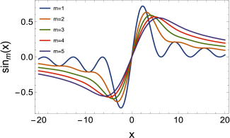
A plot of nearly sine and cosine functions is given in Figure 6 for different values of m. It seems obvious that the nearly cosine functions resemble absorption line shapes, i.e., they could represent the imaginary part of a dielectric susceptibility, while the nearly sine functions resemble the real part of a dielectric susceptibility, related to the real index of refraction of a dense medium.
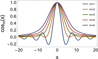
Left:
The proof of identities (A.1) can easily be achieved by noting that
Realizing that
we obtain the first of equations (A.1). The second equation is easy to prove, starting from the definition given in equation (2.6).
An analogous result has been obtained in [5], where the umbral treatment of the Gaussian functions has naturally led to the link between the ordinary Gaussian and the Dawson function.
The key element extending the Hilbert transform to these families of functions is a consequence of their UI, realized through a Lorentzian. The functions
provide the most elementary example of Hilbert transform.
B Standard deviation of nearly cosine functions
Nearly cosine functions are surely normalizable, the latter given by equation (2.4). However, it is impossible to define a standard deviation for such functions. Indeed, starting from the Lorentzian umbral image in equation (2.2), it is straightforward to see that the integral
does not converge.
Even though the previous statement sufficient for our purposes, it requires some refinements.
The Lorentzian umbral image has already been exploited to study the umbral properties of Gaussian-like functions. The ordinary Gaussian has indeed been defined as (see [5])
Accordingly, the second-order moment can be defined as
The evaluation of the previous integral is as follows:
Noting that
we finally obtain
which seems to contradict the previous statement. The subtle point is that the derivation of the integral in equation (B.1) is based on the following assumptions:
the vacuum can be brought outside the integral,
the integration over s and x can be inverted,
which holds for forms of the umbral operator that allow the convergence of the integral under study [11, 5, 2]. This last point deserves further investigation and will be discussed with more details elsewhere.
References
[1] L. C. Andrews, Special Functions of Mathematics for Engineers, 2nd ed., Oxford University, Oxford, 1998. 10.1093/oso/9780198565581.001.0001Search in Google Scholar
[2] D. Babusci, G. Dattoli, S. Licciardi and E. Sabia, Mathematical Methods for Physicists, World Scientific, Hackensack, 2020. 10.1142/11315Search in Google Scholar
[3] W. Colson, C. Pellegrini and A. Renieri, Free Electron Laser Handbook, Elsevier, Amsterdam, 1990. Search in Google Scholar
[4] J. P. Dahl and M. Springborg, The Morse oscillator in position space, momentum space, and phase space, J. Chem. Phys. 88 (1988), no. 7, 4535–4547. 10.1063/1.453761Search in Google Scholar
[5] G. Dattoli, E. Di Palma and S. Licciardi, On an umbral point of view of the Gaussian and Gaussian-like functions, Symmetry 15 (2023), no. 212, Article ID 2157. 10.3390/sym15122157Search in Google Scholar
[6] G. Dattoli, E. Di Palma, S. Licciardi and E. Sabia, From circular to Bessel functions: A transition through the Umbral method, Fractal Fract. 1 (2017), no. 1, Paper No. 9. 10.3390/fractalfract1010009Search in Google Scholar
[7] G. Dattoli, M. Haneef, S. Khan and S. Licciardi, Unveiling new perspectives of hypergeometric functions using umbral techniques, Bol. Soc. Mat. Mex. (3) 30 (2024), no. 3, Paper No. 77. 10.1007/s40590-024-00657-wSearch in Google Scholar
[8]
L. Euler,
De radicibus aequationis infinitae
[9] I. S. Gradshteyn, I. M. Ryzhik and R. H. Romer, Tables of integrals, series, and products, Am. J. Phys. 56 (1988), Paper No. 958. 10.1119/1.15756Search in Google Scholar
[10] A. Gray and G. B. Mathews, A Treatise on Bessel Functions and Their Appliations to Physics, Macmillan, New York, 1895. Search in Google Scholar
[11] S. Licciardi and G. Dattoli, Guide to the Umbral Calculus—A Different Mathematical Language, World Scientific, Hackensack, 2022. 10.1142/12804Search in Google Scholar
[12] S. M. Roman and G.-C. Rota, The umbral calculus, Adv. Math. 27 (1978), no. 2, 95–188. 10.1016/0001-8708(78)90087-7Search in Google Scholar
[13] D. Royer, Bonding Theory, McGraw-Hill Ser. Undergrad. Chem., McGraw-Hill, New York, 1968. Search in Google Scholar
[14] C. E. Sandifer, How Euler Did It, MAA Spectrum, Mathematical Association of America, Washington, 2007. 10.1090/spec/052Search in Google Scholar
[15] C. J. Sangwin, An infinite series of surprises, Math. Plus Magazine 1 (2001). Search in Google Scholar
[16] J. S. Toll, Causality and the dispersion relation: Logical foundations, Phys. Rev. (2) 104 (1956), 1760–1770. 10.1103/PhysRev.104.1760Search in Google Scholar
© 2025 Walter de Gruyter GmbH, Berlin/Boston