Optimized AVHRR land surface temperature downscaling method for local scale observations: case study for the coastal area of the Gulf of Gdańsk
-
Andrzej Chybicki
 and
Zbigniew Łubniewski
and
Zbigniew Łubniewski

Abstract
Satellite imaging systems have known limitations regarding their spatial and temporal resolution. The approaches based on subpixel mapping of the Earth’s environment, which rely on combining the data retrieved from sensors of higher temporal and lower spatial resolution with the data characterized by lower temporal but higher spatial resolution, are of considerable interest. The paper presents the downscaling process of the land surface temperature (LST) derived from low resolution imagery acquired by the Advanced Very High Resolution Radiometer (AVHRR), using the inverse technique. The effective emissivity derived from another data source is used as a quantity describing thermal properties of the terrain in higher resolution, and allows the downsampling of low spatial resolution LST images. The authors propose an optimized downscaling method formulated as the inverse problem and show that the proposed approach yields better results than the use of other downsampling methods. The proposed method aims to find estimation of high spatial resolution LST data by minimizing the global error of the downscaling. In particular, for the investigated region of the Gulf of Gdansk, the RMSE between the AVHRR image downscaled by the proposed method and the Landsat 8 LST reference image was 2.255°C with correlation coefficient R equal to 0.828 and Bias = 0.557°C. For comparison, using the PBIM method, it was obtained RMSE = 2.832°C, R = 0.775 and Bias = 0.997°C for the same satellite scene. It also has been shown that the obtained results are also good in local scale and can be used for areas much smaller than the entire satellite imagery scene, depicting diverse biophysical conditions. Specifically, for the analyzed set of small sub-datasets of the whole scene, the obtained RSME between the downscaled and reference image was smaller, by approx. 0.53°C on average, in the case of applying the proposed method than in the case of using the PBIM method.
1 Introduction
Remote multispectral sensing is an important tool for environment monitoring that has several applications in industry and science. Particularly, satellite thermal-infrared observations (TIR) are of high importance as they allow for observing and analyzing several physical and other phenomena that take place in the Earth’s environment, namely air-soil heat fluxes, atmospheric processes and vegetation changes, radiation processes, evapotranspiration and other phenomena in global, regional and local scales.
When taking the data quality and its applications into account, several criteria can be considered, such as spatial resolution, time resolution (the revisit time), data accuracy, spectral resolution, etc. Due to technical constraints, it may be said that each Earth observation satellite system is a kind of a compromise between several criteria mentioned above. In order to reduce the drawbacks of low quality of a particular sensor in one aspect, other sensors can fill the gap in another aspect in order to provide the most comprehensive overview on the Earth’s environment. Thus, low spatial resolution meteorological satellites provide global information on the state of the atmosphere and are characterized by a relatively short revisit time. Others, such as LANDSAT or Sentinel-2, are used mainly for high resolution land monitoring. Since the spatial and temporal resolution of TIR imaging systems are negatively correlated, an approach based on subpixel mapping of the Earth’s environment is of high interest.
Subpixel mapping relies on combining the data retrieved from sensors at different spatial and time resolution in order to generate products which would combine the advantages of products that they have been generated from. The retrieved datasets are a combination of high spatial resolution imagery with datasets characterized by lower spatial resolution but being more frequently registered. The combination of both sources yields a new quality in observation products because the data is frequently delivered and has higher spatial resolution. As a consequence, this enables the potential use of low resolution thermal datasets in observing phenomena at a higher scale, such as microclimate studies, human activities monitoring, urban heat island effects observations [1], urban and peri-urban areas canopy characterization or local water containers quality monitoring [2, 3]. Moreover, it enables for better understanding of and identifying processes of urban and sub-urban heat balance and better characterization of urban microclimate changes [4].
Despite the long history of available LST generated from space-borne observations, recent activities aiming to remove barriers related to low resolution observations are of considerable interest. There are several approaches in the literature that aim to construct synergistic methods exploiting information from time- and spatial-multiresolution datasets in order to retrieve the sub-scale spatial information about an observed area. For instance, Kustas et al. [5] proposed a coarse resolution temperature disaggregation method based on vegetation indices and surface radiometric temperature validated by a sensing-based energy balance model over US Southern Great Planes. G. Yang [6] proposed a method of imagery downscaling based on endmember function remote sensing indices calculated from the reflectivity data of ASTER VNIR/SWIR wavebands and land cover types database, processed with the genetic algorithm and self-organizing feature map artificial neural network (GA-SOFM-ANN) for heterogeneous area of Changping District, located on the northeast of Beijing City, China. Many approaches are also focused on urban area LST downscaling like M. Stathopoulou [7], who sharpened AVHRR thermal images and derived daily LST of 250-m spatial resolution for four cities in Greece, or Mitraka et al. [8], who focused on urban and suburban areas of Heraklion, Greece. Also, Bechtel et al. [9] downscaled SEVIRI data by a factor of two for monitoring UHI in Hamburg, Germany, while Keramitsoglou et al. [10] tested different regression algorithms for the same purpose over the area of Athens, Greece. Other approaches rely on estimating high resolution features directly by models that have been trained on, or calibrated to training datasets [11–14], or on utilizing soft-classification procedures to estimate the degree of membership of each pixel with respect to each of the end-member classes. Methods that rely on using artificial neural networks [15], fuzzy classifiers [16–18], or Adaptive Subpixel Mapping Based on a Multiagent System [19] can be also found in the literature.
The approach [13] that uses a linear mixture model based on the assumption that the spectral response xk of a pixel k is a linear weighted sum of spectral responses of its component classes expressed by:
where M is a q by c matrix in which q represents the number of wavebands and c the number of classes, the term f represents a vector, of length c, that expresses the proportional coverage of the classes in the area represented by a pixel, and e is a term that represents the vector of errors, is to some extent most similar to our methodology. The columns of the matrix M are end-member spectra, essentially the characteristic spectral responses of the classes.
However, in our study we do not use a set of spectral responses for high resolution pixels, but instead we utilize a sub-sampling kernel retrieved from a high resolution scene that describes quasi-stable radiometric properties of the land surface, namely, the effective emissivity derived from the land cover map type and vegetation index in the form of fractional vegetation cover (FVC). In particular, we assume that estimation of LST high resolution value should be done with taking into account the local effective emissivity high resolution value, but not necessarily with an assumption of the global linear dependency between emissivity and LST like in the PBIM method [20] (subsection 2.2), as suggested by Jiang and Islam [21, 22]. Instead, we introduce and estimate a vector of weights that permits more flexible, and adjusted to local conditions, modeling of dependency between emissivity and LST. This vector of weights is estimated by the so-called inverse downscaling process using the inverse problem approach and utilizing the Tikhonov regularization method.
The proposed algorithm generates a land surface temperature product characterized by high spatial resolution (≈ 100 m) derived from AVHRR imagery, thus having increased revisit frequency. The proposed approach relies on finding an optimal dataset that minimizes differences between the generated downscaled product and original low resolution scene (≈ 1.1 km at nadir). The validation of the process is based on comparing the generated downscaled product 100 m high resolution image to Landsat 8 TIRS 100 m LST products registered at the same time. The proposed approach can be applied operationally since the inverse problem approach finds an optimal solution to the problem, in the sense of the mean-square error (MSE). However, operational application of the method requires the prior, detailed analysis of its performance applied on specific region and data, therefore, The proposed algorithms of downscaling were tested and verified for the coastal zone of the Gulf of Gdansk, Southern Baltic, area of Europe.
Placing the proposed approach in the context of the existing solutions of the mentioned problem, it may be noted that most of the downscaling techniques used utilize a quasi-optimal assumption of dependence between the high resolution kernel (i.e. effective emissivity) and land surface temperature. This dependence is usually computed on the basis of radiative transfer models, is determined empirically or calculated with the use of neural networks [23] or fuzzy logic computing schemes. Because of the issues mentioned above, most of the approaches presented in the literature are not self-adaptive because they require additional information retrieved from external models. What is more, regarding the approaches based on soft computing techniques, like neural networks or fuzzy logic, a computational model used in such cases to calculate the given quantity for fine scale pixels in the course of the downscaling process, is to large extent arbitrary and may not correspond to the physics of the underlying phenomena.
The advantage of the proposed method over the existing approaches is that it finds an optimal solution to the stated problem. In order to present the advantages of the proposed approach, we have compared the obtained results with those achieved using one of the most popular methods - namely the PBIM.
2 Problem formulation and solution concept
2.1 Downscaling theory
Downscaling is the process of converting a set of spatial information (e.g. 2- or 3-dimensional) from a low to a high resolution. In the context of LST estimation based on satellite imagery, downscaling refers to estimation of LST values within the sub-pixel area. In practice, in order to downscale a satellite image, thus improving its spatial resolution, the approach of merging at least two datasets is used; a low resolution image is merged to a high resolution image (from the same or different sensor), or a low resolution image obtains spatial details of a high resolution image [24, 25].
According to the downscaling principles, the proposed approach assumes to retain radiometric characteristics of input images and aims to minimize the error. Let us assume two input data sources - such that both sources represent acquisition over the same area, and that a physical quantity they measure is comparable, i.e. they measure the same quantity in the same units (energy, radiance, temperature, etc.). Another point in the methodology is the definition of relation between two data sources that enables transformation from one source domain to another. Both sources have different but spatially constant resolution (Fig. 1).

Diagram representing the relation between the spatial distribution of measured quantity in high resolution and low resolution
Let us assume that for a given flat area, corresponding to a pixel in coarser resolution, the value of measured quantity is the weighted average of this quantity for all subareas corresponding to pixels in finer resolution contained by the coarse resolution pixel area. It is mathematically expressed as:
where
where
Tlow - is the value of the pixel in coarse resolution,
s(n) - is the area of the given pixel in high resolution,
S - is the area of a single pixel in coarse resolution,
N - is the number of pixels in high resolution imagery that are contained in the corresponding pixel of low resolution image.
In general, N depends on the ratio of data sources’ spatial resolution taken under consideration and may also depend on the number of high resolution pixels being excluded from the analysis for a given low resolution pixel due to cloud presence and other limitations.
The dependency mentioned above enables transformation between the high and low scale. However, as the transformation of pixel values from the high to low scale results in the loss of information, the reverse transformation is obviously ambiguous. The estimation of pixel values of high resolution having given pixel values of low resolution requires some additional, local, high scaled information about characteristics of the specific area that influences the pixel values Tlow and Thigh, i.e. some independently measured quantity Q usually derived from satellite imagery or auxiliary database as well. The influence of Q on T ought to be stable, which means that the dependence between Q and PV should be the same for the entire investigated area. Also, Q values should be stable in time (to a higher degree than the quantity expressed by PV), which makes it easier to collect them (i.e. lower satellite revisit time is needed). In the case of LST as T, the surface thermal properties expressed by its vegetation index or effective emissivity may be used as Q [26]. The latter was utilized by the authors in the current study. One of the main assumptions applied is that the generalization of the rule connecting the local emissivity and LST value must be allowed with respect to at least a single scene of low resolution imagery.
The way of utilizing the high resolution information on thermal properties of the land for downscaling the LST image is described in the next subsections.
2.2 PBIM method
Having defined the concept of downscaling, let us focus on the particular method of downscaling to be optimized. Since the objective of the study is to present the optimized downscaling AVHRR LST method in view of its applicability in coastal zone LST estimation, we have taken under closer analysis the PBIM (Pixel Block Intensity Modulation) downscaling process, described in the next subsection, and proposed a way of its optimization.
PBIM is proposed for downscaling thermal products to higher resolution using the high resolution transformation kernel. The general form of the PBIM method is expressed as:
where Tlow - is the pixel value of the image in low resolution, εhigh - is the high effective emissivity pixel value, εhigh→mean - is the high effective emissivity value averaged for a current low resolution pixel area, Thigh - is the resulted current pixel value of high resolution downscaled image. It should be noted that according to formula (4), the strict linear relation between ε and T is assumed.
The appropriate definition of the used high resolution data source, referred to here as ε, is the most important issue in the utilized downscaling method. The better the description of local properties of the area the image of which is to be downscaled, the smaller the obtained error of transformation. The effective emissivity composite product values calculated based on several high resolution images were utilized as the HRK [27].
The PBIM allows for merging multiresolution 2D datasets retrieved from sensors. Note that in this approach, the simulated high resolution image retains the radiometric characteristics and spatial distribution of the original low resolution image. In particular, the average of the simulated high-resolution sub-pixel values is equal to the pixel value of the original low resolution image.
The PBIM method can be applied to any satellite imagery derived products - from a relatively low level, where pixel values are spectral bands of the images, to higher levels like LST or SST products.
Note also that in this approach to re-scaling of thermal products it is important that spatial data considered for processing must represent relatively flat areas, thus the low scale can be expressed as a simple aerial average of the LSTs at the high scale [28]. Also, the re-scaling methods have limitations for areas with high surface type diversity, which particularly refers to wetlands, water containers situated among sub pixel areas. Water surfaces have different emissivity and heat capacity properties and thus they significantly influence the model [29].
2.3 Proposed method of PBIM optimization
In the presented approach, as in the PBIM method, the εhigh also plays a principal role, as it describes high resolution properties of an area corresponding to LST image to be downscaled. As mentioned, εhigh is computed based on high resolution quasi-static data that describes thermal properties of an area. The choice on what should be the basis for the construction of εhigh used for defining the rescaling transformation is somewhat arbitrary. The general rule is that it should possibly describe the thermal properties of the surface in the best possible way - particularly the surface’s susceptibility to absorb heat from shortwave radiation if the aim is to downscale day-time LST [30]. Also, what has been introduced in subsection 2.1, εhigh is considered to be quasi-static and much easier to be retrieved than data to be downscaled [31]. Note also that images used to construct composite data must be registered in similar vegetation and weather conditions [32]. In our approach, we have taken under consideration the summer period of the years of 2013 and 2014. The FVC and subsequently the effective emissivity ε have been calculated on the basis of the normalized differential vegetation index (NDVI) using the formulae (20) and (21) from subsection 3.2.
What is more, as mentioned in the previous section, the PBIM method relies on a relatively simple assumption that Thigh depends linearly on the respective values (eq. 4). It can be observed that this is not always the case [33]. For instance, Fig. 2 presents the plot of effective emissivity from Landsat 8 OLI vs. corresponding values of LST from Landsat 8 TIRS for the investigated Pomerania region in Northern Poland (for details on data processing, and specifically on effective emissivity and LST calculating from Landsat 8 imagery – see section 3). The content of Fig. 2 is in general in line with the known observations of the “triangle” character of the VI – LST dependence. Fig. 2b shows the relation between effective emissivity values, namely, the central values of particular small ranges of effective emissivity, and LST values averaged for groups of pixels corresponding to those effective emissivity small ranges (red points). It is able to be seen from the figures that the relation between effective emissivity and LST tends not to be linear. The line of fit (corresponding to all data presented in Fig. 2a, not only to averaged data from Fig. 2b) is shown in Fig. 2b by black dots. It is visible that it cannot be used as a satisfactory approximation of εhigh - LST dependence.

LST/effective emissivity scatter plot for considered area (a). Right picture (b) represents effective emissivity and LST dependence for considered region: red plot vs. LST value represents averaged for groups of pixels corresponding to small ranges of effective emissivity. Black plot is a linear approximation of effective emissivity and LST dependence.
To take into account the non-linear dependence between the biophysical properties of the surface in the LST downsampling, the authors propose the following inverse downscaling approach (DSopt). We assume that there exists a dependence between effective emissivity and LST expressed as
where f (·) need not to be linear (and does not have to be monotonic as well), and may be estimated for instance as the red plot in Fig. 2. Combining (2) and (5), and naming PV explicitly as LST, yields:
for a given low scale pixel. The form of f (·) is generally unknown for a given terrain, but assuming that it is stable for the entire scene and applying (6) to each low scale pixel, we may express the problem as a system of linear equations. For this purpose, let us calculate the histogram [h1, h2, ..., hK] of εhigh (where hk, k = 1, ..., K is the percentage of high scale pixels whose εeff value belongs to a given range) for each low scale pixel, using always the same εeff minimum/maximum values and the same number of bars K. Then, if we express f (·) as a vector of values (weights) [w1, w2,...,wK] corresponding to the central values of εeff ranges used in calculating the histogram, and assuming that the single pixel area Sn is constant, we may write (6) as
where m is the number of a “coarse” pixel in a scene (m = 1,..., M). The system of M equations (7) may be also written in a matrix form:
and may be shown as a diagram – Fig. ??.
Referring to (7) and (8), each row in H matrix represents information on thermal properties of terrain within a certain pixel of low resolution image (Fig. 3). Row values of H represent histogram values calculated using a corresponding set of N pixel values of εeff from high resolution image (in reality, usually less than N pixel values is used for a given coarse pixel, due to cloud presence or other limitations in high scale data from which εhigh has been derived). LSTlow is a column vector containing low resolution image LST values and w is the vector of weights to be found. Having two data sources (LST in a coarse scale and εhigh in a fine scale) which fulfil the conditions stated above, for the whole scene a set of M equations with K variables is obtained.

Diagram of matrix equation representing dependence between high and low resolution datasets
Finally, as wk values express the LST themselves, after finding them with use of the method described in the next subsection, the LSThigh may be estimated directly as wk corresponding to a given εhigh value, or with the application of some kind of interpolation of w values.
2.4 Finding an optimal solution
Now our task is to estimate w having given LSTlow and H. Let us denote the observation vector LSTlow as y and the searched vector of parameters w as x, and include the vector v of bias which is always present in a real measurement situation:
Estimation of x having known H and measured y biased by unknown v is a typical linear inverse problem [34]. Unfortunately, in reality we usually have to take into account that the postulated model does not describe the relation between x and y perfectly, e.g. it is linear only in approximation, or the assumed values in H are not fully correct, or the assumed number of independent variables (the number of x elements) is not correct. Moreover, the K and M values are not equal and thus H matrix is not invertible. Thus, one of the possible ways to obtain the solution in such a situation is to estimate x in a sense of least squares, i.e. by minimizing the ∥Hx − b∥2 where ∥ · ∥2 is the Euclidean norm. Estimate
if the HTH matrix is not singular. In such a case, a regularization term is introduced to provide the existence of the solution, changing (10) to:
where Γ is a suitably chosen Tikhonov matrix [35-38] and x0 is the expected solution calculated from the PBIM method. We used the simple form of Γ = λI, where I is the identity matrix and the λ value was found using the nearoptimal parameter calculation of singular value decomposition method proposed by O-Leary [34].
The solution
At the last step of the proposed approach, the image is reconstructed to high resolution using optimal weights stored in
where:
-
3 Experimental setup
3.1 The experiment scheme and data flow
In order to compare the results obtained using the proposed approach with other existing solutions, we used two basic types of datasets: AVHRR and Landsat 8, registered at possibly the same time. Then, we assumed that AVHRR LST is a low spatial resolution (1.1 km) input data that is downscaled to higher resolution (100 m) and we treat Landsat 8 LST product as a kind of proxy validation dataset.
In this case, the effective emissivity, as the static high resolution data to be merged with low resolution image, was retrieved from a composition of two Landsat 8 images registered on 2013-08-05 at 09:45:37 UTC (scene center time) and on 2014-07-23 at 09:43:29 UTC (scene center time). For both of the scenes, fractional conditions for the analyzed area are similar (middle of the summer) and repeatable. The Metop-B/AVHRR3 imagery was registered on 2013.08.05 on 9:10:26 UTC.
The overview diagram of processing and validation strategy of the proposed approach is presented in Fig. 4. After creating the composite FVC high resolution image from two Landsat 8 scenes, it was used along with the AVHRR low resolution LST image as an input to our downscaling procedure. Also, for comparison of the results, the PBIM downscaling was applied for the same data. At the end, a comparison of the down-scaling results, obtained both by DSopt and PBIM with the high resolution Landsat 8 LST data, was performed.

Overall diagram of data processing flow and verification
It should be noted that for Landsat 8, in the climatic zone of the considered region several requirements need to be fulfilled to provide the appropriate analysis. The acquisition should be made under clean sky conditions in order not to interfere with the values registered in thermal and visible channels. The presence of clouds, aerosols, and diverse spatial distribution of water vapor content highly disturbs the process of acquisition. Also, note that Landsat 8 was launched in 2010 and together with a long revisit time (16 days), it highly reduces the number of available acquired imageries where all conditions stated above can be met.
We also performed accurate geometric calibration of both data sources to provide a unified reference system and cover the same areas of analysis. Data from both sources were reprojected to UTM zone 34 projection where the imageries cover area from 271872 to 434655 easting and 6004014 to 6092171 northing based on WGS 84 ellipsoid. The whole area covers 14,256 km2, in which land consists of about 51% of the data. The height of the terrain is not moderately diverse as most of it is covered by flat areas or small hills. Diverse vegetation conditions of the urban areas of Gdańsk, Sopot and Gdynia municipality (Tricity), and green areas (forests, farmlands) located nearby, cause the NDVI to vary from approx. 0.12 to 0.67.
Fig. 5 presents the map of the location of the area of interest: the land at the Gulf of Gdańsk, Southern Baltic Sea in Poland, along with LST maps calculated using imageries from both sensors – high resolution Landsat 8 and low resolution MetopB/AVHRR.
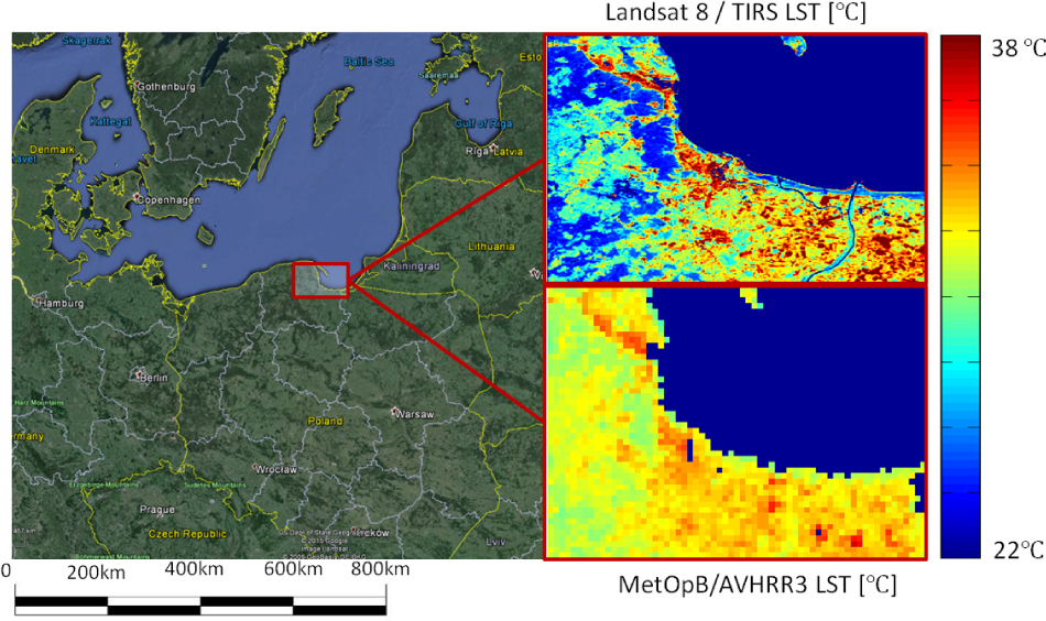
On the left: the map depicting the location of the area of interest – the Gulf of Gdansk, South Baltic, Poland (source: Google Earth), on the right: LST maps calculated from both sensors – Landsat 8/TIRS (top-right) and MetopB/AVHRR3 (bottom-right). Blue pixels in the upper and the lower right images represent sea or cloud areas that were masked out of the analysis.
3.2 LST estimation
In the study, we selected MetOp-B/AVHRR3 imageries as the source of low resolution data to be downscaled and Landsat 8/TIRS LST as a validation dataset.
The set of NOAA and MetOp satellites utilizes the AVHRR radiation-detection moderate resolution remote imager dedicated to land and atmosphere. Due to quite a large number of currently operating NOAA and MetOp satellites, the AVHRR sensor is characterized by a relatively high time resolution (the revisit time for the respective region is approx. 2-3 hours). Tab. 1 presents the characteristics of AVHRR channels according to NOAA KLM User’s Guide.
Characteristics of AVHRR spectral channels
| Channel Number | Resolution at Nadir | Wavelength (µm) | Typical Use |
|---|---|---|---|
| 1 | 1.09 km | 0.58-0.68 | Daytime cloud and surface mapping |
| 2 | 1.09 km | 0.725 - 1.00 | Land-water boundaries |
| 3A | 1.09 km | 1.58-1.64 | Snow and ice detection |
| 3B | 1.09 km | 3.55-3.93 | Night cloud mapping, sea and land surface temperature |
| 4 | 1.09 km | 10.30 -11.30 | Night cloud mapping, sea and land surface temperature |
| 5 | 1.09 km | 11.50 -12.50 | Sea and land surface temperature |
| REVISIT TIME: 8 per day | |||
As it is known, LST estimation requires emissivity correction [39-42]. Therefore, during this process we calculate the average emissivity for 4th and 5th AVHRR channel, denoted as εAVHRR and the difference of these channels’ emissivity ΔεAVHRR. The calculation process was different for several NDVI ranges. Namely, for NDVI < 0.2 the pixel is considered to be bare soil, then:
where R1 is AVHRR channel 1 reflectance.
Pixels with 0.2 < NDVI < 0.5 are considered to be partly vegetated and the εAVHRR and ΔεAVHRR are calculated using the following formulae:
where
For NDVI > 0.5 pixel is considered to be full vegetation and εAVHRR and ΔεAVHRR is fixed as:
The validation dataset was retrieved from the Landsat 8 satellite, which images the entire Earth every 16 days in an 8-day offset from Landsat 7. Landsat 8 carries two instruments: the Operational Land Imager (OLI) sensor that includes refined heritage bands, along with three new bands with respect to Landsat 7 [43]a deep blue band for coastal/aerosol studies, a shortwave infrared band for cirrus detection, and a Quality Assessment band. The Thermal Infrared Sensor (TIRS) provides two thermal bands. Both these sensors provide improved signal-to-noise radiometric performance quantized over a 12-bit dynamic range. The improved signal to noise performance of Landsat 8 enables better characterization of the land cover state and conditions. Products are delivered as 16-bit images (scaled to 55,000 grey levels). Table 2 presents the characteristics of Landsat 8 channels.
Characteristics of Landsat 8 spectral channels
| Channel Number | Resolution at Nadir | Wavelength (µm) | Description/Typical Use |
|---|---|---|---|
| 1 | 30 m | 0.43-0.45 | Coastal aerosol |
| 2 | 30 m | 0.45-0.51 | Visible - blue |
| 3 | 30 m | 0.53-0.59 | Visible green |
| 4 | 30 m | 0.64 - 0.67 | Visible - red |
| 5 | 30 m | 0.85 - 0.88 | Near infrared (NIR) |
| 6 | 30 m | 1.57 - 1.65 | SWIR 1 |
| 7 | 30 m | 2.11 - 2.29 | SWIR 2 |
| 8 | 30 m | 0.50-0.68 | Panchromatic visible |
| 9 | 30 m | 1.36-1.38 | Cirrus detection |
| 10 | 100 m | 10.60-11.19 | Night cloud mapping, sea and land surface temperature |
| 11 | 100 m | 11.50-12.51 | Sea and land surface temperature |
| REVISIT TIME: 16 days |
The LST from Landsat 8 imagery was calculated by applying the split window technique algorithm that uses two thermal bands located in the atmospheric window between 10 and 12 µm. Then, we applied radiometric calibration procedure for Landsat 8 data using metadata of the provided imagery and used expansion of the Planck equation according to (17) for TIRS data. Spectral radiances delivered in Landsat datasets were converted into satellite brightness temperature using the following relationship [44, 45]:
where:
K1 - band specific thermal conversion coefficient delivered with Landsat 8 imagery metadata files, namely K1 = 774.89 for channel 10 and 440.89 for channel 11
K2 - band specific thermal conversion coefficient delivered with Landsat 8 imagery metadata files, namely K2 = 1321.08 for channel 10 and 1201.14 for channel 11
TOAi - top of the atmosphere spectral radiance
Landsat 8 LST emissivity correction, denoted as εTIRS, was performed according to a procedure proposed by Skokovic et al. [46], Shaouhua Zhao et al. [47], according to the values presented in the Tab. 3, with use of the Corine Land Cover database and FVC data, in order to distinguish urban and non-urban area.
Emissivity values for urban and non-urban areas for TIR bands
| Emissivity | Band 10 | Band 11 |
|---|---|---|
| Land surface emissivity of urban area | 0.971 | 0.977 |
| Land surface emissivity of non - urban area | 0.987 | 0.989 |
The split window technique (SWT), utilizing the thermal channels of AVHRR3 and TIRS, has been used here for LST calculation. This is a relatively simple and robust method of retrieving LST estimation for large or regional scale applications. Its main property is that it removes atmospheric fluctuations, taking advantage of the fact that radiation absorption differs in particular wavelengths of electromagnetic spectra. Consequently, the TIRS and AVHRR LST images were corrected pixel by pixel for emissivity and water vapor content, according to Jimenez-Munoz [48–51] with values of c0-c6 (Tab. 4) according to the following formula:
Effective wavelengths for thermal channels used in SW technique and equation coeflcients applied for LST estimation procedure for AVHRR and OLI
| Platform/senser | λi–λj | c0[K] | c1[-] | c2[K–1] | c3[K] | c4[K cm2g–1] | c5[K] | c6[K cm2g–1] |
|---|---|---|---|---|---|---|---|---|
| METOP B/AVHRR3 | 10.82-11.97 | −0.045 | 1.733 | 0.307 | 44.3 | 0.61 | −150 | 18.7 |
| Landsat 8/TIRS | 10.8-12 | −0.268 | 1.378 | 0.183 | 54.3-2.238 | −129.2 | 16.4 |
where W is a water vapor content retrieved from an external database [50–54], Ti and Tj are thermal channels of AVHRR (i = 4 and j = 5) and TIRS (i = 10 and j = 11) respectively,
With the above consideration in mind, in our methodology we proposed the following approach:
we applied the split window technique for MetopB/AVHRR3 and for Landsat 8 TIRS,
in both algorithms we used the surface emissivity and water vapor content correction approach.
Effective emissivity ε computation was based on high resolution NDVI data over the respective region. The maximum NDVI (NDVImax) and the minimum NDVI (NDVImin) values for the study area were determined, which were further used for computing the fractional vegetation cover (FVC) [57, 58]:
and the effective emissivity ε as:
4 Results
4.1 Comparison of LST downscaling results for the entire scene
In this subsection we present the results obtained using the proposed optimized downscaling process of LST. We compared the results obtained by DSopt with the PBIM method of downscaling in global (i.e. for the entire scene Fig. 6, and using a more detailed analysis in Fig. 7) and local scale (i.e. for the locations along the two selected transect lines within the investigated land area, Fig. 8, 9 and 10) using objective criteria, namely, the root mean squared error (RMSE) and the Pearson correlation coefficient (R). Pixels representing either clouds or sea on any of the images were masked during the analysis so their values did not interfere with the overall process of error minimization.
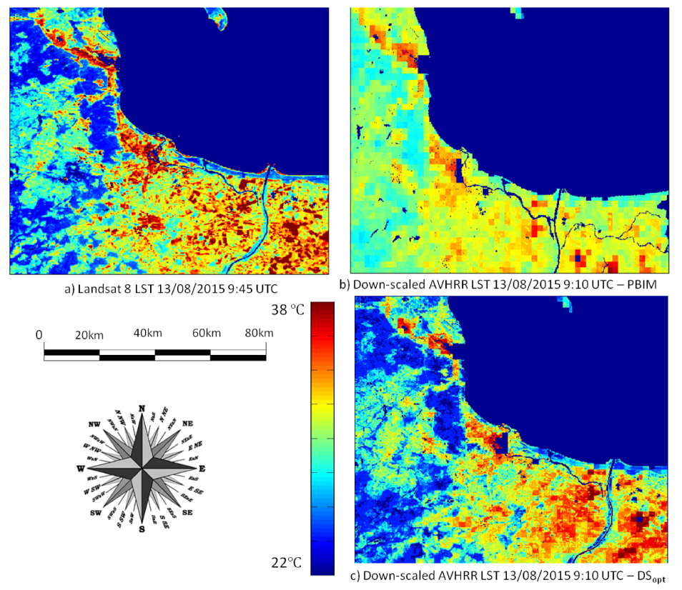
Comparison of downscaling results for the investigated area: top-left: LST calculated from Landsat 8 image, top-right: LST downscaled from AVHRR using PBIM method, bottom-right: LST downscaled from AVHRR using DSopt method

The obtained downscaled to high resolution AVHRR LST image and scatter plot (every 100th point) of Landsat 8 LST and downscaled AVHRR LST (right) using DSopt. Red line in right image represents “1:1” line. Correlation coeflcient and root mean squared error (RMSE) were: R=0.828 and RMSE=2.255°C, respectively.

Landsat LST image with marked two transect lines defining the small subareas selected for detailed analysis of the downsampling results. The first line (AB) starts from suburban areas of the Tricity municipality (A), passes through a vegetated area of the Tricity Landscape Park and ends in the Tricity municipal area near the border between Gdańsk and Sopot (B). The second transect starts from the suburban area of Gdynia (C), passes through forest areas and ends in the center of Gdynia city (D).

Comparison of LST high resolution data with respect to AB transect line: Landsat 8 LST, AVHRR LST downscaled by DSopt method, AVHRR LST downscaled by PBIM method and AVHRR LST downscaled by nearest neighbor technique

Comparison of LST high resolution data with respect to CD transect line: Landsat 8, AVHRR DSopt downscaled by the proposed method, AVHRR downscaled by the PBIM method (AVHRR PBIM) and AVHRR resampled to LANDSAT 8 resolution using nearest neighbor technique
We compared the obtained downscaled high resolution image to LST calculated from Landsat 8 image acquired on 13 August 2013. The RMSE between Landsat 8 LST and downscaled image using DSopt was 2.255°C with correlation coefficient R equal to 0.828 and Bias = 0.557°C. It shows a significant improvement in comparison to the PBIM method, where we obtained RMSE = 2.832°C, R = 0.775 and Bias = 0.997°C.
The analysis of spatial distribution images shows that the results obtained by DSopt algorithm better represent thermal characteristics for the analyzed area and are visually closer to the original Landsat 8 LST image than the image obtained using the PBIM method (Fig. 6). Specifically, it can be observed that the influence of local surface high resolution characteristics is reflected in DSopt rather than local LST retrieved from AVHRR observations. What is more, as in the PBIM, the LSTlow term is directly used in the formula and strongly influences the obtained LSThigh value, it results in the appearance of coarse resolution artifacts in the downscaled product (Fig. 6b). This effect does not occur in the DSopt result case. In Fig. 7 we presented the scatter plot of this case.
4.2 Detailed analysis of the retrieved results
In many cases, for instance for small areas where we deal with high diversity of surface conditions, obtaining the local accurateness of the applied downscaling is even more important. For this purpose, we took under consideration two relatively small sub-areas defined as narrow strips of land situated along selected “cross section” lines, in order to verify how the algorithm manages with diverse heterogeneous conditions (Fig. 8).
The first line starts from the West, at point A located at 53.9356°N, 17.6832°E, which is situated in the suburbs of the Tricity area. Then, the line transects through the Tricity Landscape Park and ends in the urban area of the Tricity municipality (Gdańsk-Oliva district) - point B (53.9309°N 17.8077°E). The length of the line is 6 km and it transects through low as well as very high vegetated areas, so the thermal conditions along this transect are significantly diversified.
The second line starts from suburban area of Gdynia (point C – 54.045 °N, 17.6513 °E), passes through forest areas and ends in the center of Gdynia city (point D – 53.9544 °N, 17.6601 °E). The diversity of thermal conditions for the area along the second transect is quite similar to that in the case of the first line.
Afterwards we performed analysis of the obtained results along selected transects from four datasets, namely:
LST calculated from Landsat 8 TIRS dataset (validation dataset),
AVHRR LST image downscaled using the proposed DSopt method,
AVHRR LST image downscaled using the PBIM method,
AVHRR LST image downscaled transformed (resampled) to high resolution by simple nearest neighbor method.
Plotted LST high resolution values taken from particular datasets along the AB and CD transect, respectively are presented in Fig. 9 and 10. Tables 5 and 6 contain the comparison of the correlation coefficient and RMSE between Landsat 8 LST and the results retrieved by different methods of AVHRR LST downscaling: DSopt proposed by the authors, PBIM, and nearest neighbor for AB and CD transect, respectively.
Comparison of the results obtained by different downsampling methods for the subarea indicated by AB transect
| Downsampling method | Correlation coefficient R with respect to Landsat 8 LST | RMSE [°C] with respect to Landsat 8 LST | BIAS [°C] with respect to Landsat 8 LST |
|---|---|---|---|
| DSopt | 0.9334 | 2.0042 | 1.3529 |
| PBIM | 0.8207 | 2.6851 | 0.3939 |
| Nearest neighbor | 0.7544 | 2.8757 | 0.4034 |
Comparison of the results obtained by different downsampling methods for the subarea indicated by CD transect
| Downsampling method | Correlation coefficient R with respect to Landsat 8 LST | RMSE[°C] with respect to Landsat 8 LST | BIAS[°C] with respect to Landsat 8 LST |
|---|---|---|---|
| DSopt | 0.842 | 2.3927 | 1.7932 |
| PBIM | 0.6038 | 2.5262 | 0.4812 |
| Nearest neighbor | 0.5101 | 2.659 | 0.4581 |
For this relatively small area, the above results show that the optimization method presented in DSopt algorithm yields significantly better results than other approaches. Note that the aim of using the inverse problem algorithm is to minimize the downscaling error in a global, i.e. the entire imagery scale, so results corresponding to local sub-datasets do not always have to be better than when using other methods. However, this case shows that data obtained by the DSopt fits the original Landsat 8 LST the best, which serves here as a kind of proxy verification tool.
As shown above, the obtained downscaled products retain radiometric characteristics of original images for the whole imagery, however, for subdatests the BIAS results suggest that some deviation from this rule occurs. Moreover, the correlation coefficients and RMSE indicate that DSopt technique yields results closer to the original highresolution spatial pattern than the PBIM method. A more detailed investigation of the selected transect cross sections of the analyzed area indicates that also for small sub-datasets the usage of DSopt is justified as the RMSE error is reduced from 2.6851°C for the PBIM case to 2.0042°C for AB transect and from 2.5262°C to 1.5401°C for CD transect. The improvement of the proposed methodology is further verified by correlation between downscaled products and time-coincident Landsat 8 imagery. Specifically, the correlation coefficient increases from 0.8207 to 0.9212 in the case of AB, and from 0.6038 to 0.8953 in the case of CD transect.
4.3 Optimized downscaling for local scale
In the previous subsection, we have examined and evaluated the results of downscaling using the inverse technique for the whole scene imagery and for particular transect sub-datasets. We have shown that the proposed optimization technique yields better results in comparison with the direct approach. In this section, we have taken under consideration three sub-datasets of the whole scene, which differ between each other in terms of vegetation and surface conditions, and we have verified how our approach functions in such cases. The cases taken under consideration are as follows:
Case 1 - area covering nearly 300 km2 of Gdynia municipality urban area and Tricity National Park bounded by 53.7451°N, 18.4904°E (north-west) and 53.5237°N, 18.6786°E (south-east) limits. This area is rather unique and is to large extent characterized by surface type heterogeneity typical for urban area. According to the Corine Land Cover database, 51% of the mentioned area is urban, while 49% is non-urban, high vegetation area of the Tricity National Park. The results obtained by PBIM and DSopt methods for test case 1 are shown visually in Fig. 11. The quantitative results on the obtained correlation coefficient, the RMS error and the bias for this case are shown in Table 7.

Scatterplot and visual presentation of the results retrieved by PBIM and DSopt methods for local sub-dataset test case 1
Results of downscaling using PBIM and DSopt for local sub-dataset case 1
| Downsampling method | Correlation coefficient R with respect to Landsat 8 LST | RMSE [°C] with respect to Landsat 8 LST | BIAS [°C] with respect to Landsat 8 LST |
|---|---|---|---|
| DSopt | 0.8866 | 2.0513 | 0.5092 |
| PBIM | 0.7659 | 2.9984 | 0.7295 |
| Nearest neighbor | 0.7053 | 3.1898 | 0.7295 |
Case 2 – area of the Stęzyca Lake which is a part of the Pomeranian National Park that mainly comprise vegetated areas (forests and grasslands), which constitute 99% of the surface. The area is bounded by coordinates: 53.5222°N, 17.9436°E (north-east) and 53.3807°N, 18.3026°E (south-west). The results obtained by PBIM and DSopt methods for test case 2 are shown visually in Fig. 12. The quantitative results on the obtained correlation coefficient, the RMS error and the bias for this case are shown in Table 8.

Scatterplot and visual presentation of the results retrieved by PBIM and DSopt methods for local sub-dataset test case 2
Results of downscaling using PBIM and DSopt for local sub-dataset case 2
| Downsampling method | Correlation coefficient R with respect to Landsat 8 LST | RMSE [°C] with respect to Landsat 8 LST | BIAS[°C] with respect to Landsat 8 LST |
|---|---|---|---|
| DSopt | 0.6991 | 1.6796 | 0.3998 |
| PBIM | 0.5587 | 1.8755 | 0.1742 |
| Nearest neighbor | 0.4741 | 1.9937 | 0.1742 |
Case 3 - urban area of Gdańsk municipality, bounded by 53.5281°N, 18.5208°E and 53.3891°N, 19.1395°E, that mainly comprise urban areas (over 80% according to the Corine Land Cover database). The results obtained by PBIM and DSopt methods for test case 3 are shown visually in Fig. 13. The quantitative results on the obtained correlation coefficient, the RMS error and the bias for this case are shown in Table 9.

Scatterplot and visual presentation of the results retrieved by PBIM and DSopt methods for local sub-dataset test case 3.
Results of downscaling using PBIM and DSopt for local sub-dataset case 3
| Downsampling method | Correlation coefficient R with respect to Landsat 8 LST | RMSE [°C]with respect to Landsat 8 LST | BIAS [°C] with respect to Landsat 8 LST |
|---|---|---|---|
| DSopt | 0.7204 | 2.7159 | 1.4712 |
| PBIM | 0.6473 | 3.1649 | 1.8911 |
| Nearest neighbor | 0.5956 | 3.2609 | 1.8911 |
Tables 7-9 present analytical results obtained by the proposed optimization approach, PBIM method and original AVHRR3 data resampled using the nearest neighbor technique (presented in the third row) for cases 1-3. The second column of the tables represents the Pearson correlation coefficient, while the third represents the RMSE with respect to reference LST Landsat 8 OLI dataset. The last column shows BIAS between reference dataset and a result of downscaling products, in order to verify retention of radiometric properties of the results.
The results presented in these cases show that DSopt method yields results closest to Landsat 8/TIRS validation dataset having overall lowest RMSE and highest correlation coefficient among the methods presented. This can be particularly observed for test case 1 (Tab. 7) when algorithm finds minimized error solution for a heterogeneous area, including high vegetation (low effective emissivity) and urban areas (high effective emissivity), yielding RMSE reduction up to 32% (for DSopt) and correlation increase from 0.7659 (for PBIM) to 0.8866 (DSopt). As this trend is also observed in cases 2 and 3 (Tab. 8 and Tab. 9, respectively), it may be concluded that the increase of the proposed downscaling method performance is visible for local sub-datasets.
5 Conclusions
In the paper, the process of optimization of downscaling thermal products based on low resolution (AVHRR) imagery using the inverse technique approach was presented. The authors proposed a data processing model and method that transforms the downscaling process to inverse problem. We used Tikhonov regularization when finding an optimal solution to the defined problem and showed that our approach yields better results than the other approach, i.e. the PBIM direct method.
The proposed approach aims to find estimation of high resolution imagery by minimizing the global error of the downscaling process. Nevertheless, we showed by examples that apart from global optimization, the obtained results are also very good in local scale and can be used for relatively small areas – much smaller than the entire satellite imagery scene, depicting diverse surface conditions.
It should be pointed out that applying the inverse problem approach to the downscaling process is constrained by limitations and distortions. One of the main known difficulties regarding the satellite imagery processing in general is the appropriate atmospheric correction for cloud and aerosol presence and the need to remove the effects caused by atmospheric conditions. A standard model application for cloudy days can significantly decrease its quality as clouds and aerosols absorb radiation, thus making the precise effective emissivity and LST determination difficult to obtain. Hence, when the downscaling process described in this paper aims to minimize the global error and estimate the optimal weights vector, the presence of pixels not representing precise land surface conditions can perturb the entire result very strongly. In this sense, direct methods are more resistant to that type of effects.
Another aspect of the proposed methodology is the regularization parameter value. In many inverse problems, the estimation of the appropriate regularization parameter value is of a crucial importance. In our case, the optimal value was found by using near optimal parameter calculation methods based on singular value decomposition.
The kernel of the whole transformation process is the high resolution kernel matrix - it describes thermal properties of an area to be downscaled. The appropriate definition of HRK, its resolution as well as the kind of model describing the dependence of the LST on the quantity which is expressed by HRK values, determines the quality of the retrieved results. In the presented approach, we used fractional vegetation cover values to construct the HRK, but in general the HRK may be constructed from any spatial datasets that fulfill the conditions mentioned in section 2.
The proposed methodology that utilizes the inverse problem approach is a technique that can be applied to optimize the downscaling process and it can also be used in conjunction with other downscaling approaches and methods. The method is particularly suitable for cases where local biophysical conditions significantly influence the final characteristics of LST-VI relation. It is important to notice that the proposed methodology is self-adaptive in terms of technical implementation. The method constructs the high resolution kernel without human supervision, which means that applying it to regions with other climatic and meteorological conditions should be relatively straightforward. In particular, in cases where diverse vegetation conditions areas are analyzed, methods that find the minimum error solution are of considerable interest and are usually able to generate radiometric LST product that better depicts spatial distribution of LST.
References
[1] Arnfield A. J., Two decades of urban climate research: A review of turbulence, exchanges of energy and water, and the urban heat island. International Journal of Climatology, 2003, 23, 1-26, 10.1002/joc.859Search in Google Scholar
[2] Urbański J. A., Wochna A., Bubak I., Grzybowski W., Łukawska-Matuszewska K., Lacka M. et al., Application of Landsat 8 imagery to regional-scale assessment of lake water quality. International Journal of Applied Earth Observation and Geoinformation, 2016, 51, 28-36, 10.1016/j.jag.2016.04.004Search in Google Scholar
[3] Chybicki A., Łubniewski Z., Kulawiak M., Characterizing surface and air temperature in the Balitc Sea Coastal Area using remote sensing techniques. Polish Maritime Research, 2016, .3, 3-11, 2016, 10.1515/pomr-2016-0001Search in Google Scholar
[4] Merchant C. J., Matthiesen S., Rayner N. A, Remedios J. J., Jones P. D., Olesen F. et al., The surface temperatures of the earth: steps towards integrated understanding of variability and change, Geosci. Instrumentation Methods Data Syst. Discuss. 2013, 3, 305-345, 10.5194/gid-3–305–2013Search in Google Scholar
[5] Kustas W. P., Anderson M. C., Norman J. N., French A. N., Estimating subpixel surface temperatures and energy fluxes from the vegetation index-radiometric temperature relationship. Remote Sensing of Environment, 2003, 85, 429-44010.1016/S0034-4257(03)00036-1Search in Google Scholar
[6] Yang G., Puc R., Zhaoa C., Huanga W., Wanga J., Estimation of subpixel land surface temperature using an endmember index based technique: A case examination on ASTER and MODIS temperature products over a heterogeneous area. Remote Sensing of Environment, 2011, 115(5), 15, 1202-1219, 10.1016/j.rse.2011.01.004Search in Google Scholar
[7] Stathopoulou M., Cartalis C., Keramitsoglou I., Mapping microurban heat islands using NOAA/AVHRR images and CORINE Land Cover: An application to coastal cities of Greece. International Journal of Remote Sensing, 2004, 25, 2301–2316, 10.1080/01431160310001618725Search in Google Scholar
[8] Mitraka Z., Chrysoulakis N., Doxani G., Del Frate F., Berger M., Urban Surface Temperature Time Series Estimation at the Local Scale by Spatial-Spectral Unmixing of Satellite Observations. Remote Sens., 2015, 7(4), 4139-4156, 10.3390/rs70404139Search in Google Scholar
[9] Bechtel B., Zakšek K., Hoshyaripour G., Downscaling land surface temperature in an urban area: A case study for Hamburg, Germany. Remote Sens., 2012, 4, 3184–3200, 10.3390/rs4103184Search in Google Scholar
[10] Keramitsoglou I., Kiranoudis C. T., Weng Q. Downscaling geostationary land surface temperature imagery for urban analysis. IEEE Geosci. Remote Sens. Lett. 2013, 10, 1253–125710.1109/LGRS.2013.2257668Search in Google Scholar
[11] Lewis H. G, Nixon M.S., Tatnall A. R. L., Brown M., Appropriate strategies for mapping land cover from satellite imagery, Proceedings of the 25th Annual Conference of The Remote Sensing Society, Cardiff, United Kingdom, 1999, pp. 717-724.Search in Google Scholar
[12] Lewis H. G., Brown M., Tatnall A. R. L., Incorporating uncertainty in land cover classification from remote sensing imagery. Advanced Space Research A.R.L., 2000, 26(7), 1123-112610.1016/S0273-1177(99)01128-XSearch in Google Scholar
[13] Seetle J. J., Drake N. A., Linear mixing and the estimation of ground cover proportions. International Journal of Remote Sensing, 1997, 14(6), 1559-117710.1080/01431169308904402Search in Google Scholar
[14] Williamson H. D., Estimating sub-pixel components of a semiarid woodland. International Journal of Remote Sensing, 1994, 15, 3303-330710.1080/01431169408954330Search in Google Scholar
[15] Atkinson P. M., Cutler M. E. J., Lewis H., Mapping sub-pixel proportional land cover with AVHRR imagery. International Journal of Remote Sensing, 1997, 188, 917-93510.1080/014311697218836Search in Google Scholar
[16] Mather P. M., Tso B., Classification Methods for Remotely Sensed Data. Taylor and Francis, 200110.1201/b12554Search in Google Scholar
[17] Fisher P. F., Pathirana S., The evaluation of fuzzy memberships of land cover classes in the suburban zone. Remote Sensing of Environment, 1990, 34, 121-13210.1016/0034-4257(90)90103-SSearch in Google Scholar
[18] Foody G. M., Approaches for the production and evaluation of fuzzy land cover classifications from remotely-sensed data. International Journal of Remote Sensing, 1996, 17, 1317-134010.1080/01431169608948706Search in Google Scholar
[19] Xiong Xu, Yanfei Zhong, Adaptive Subpixel Mapping Based on a Multiagent System for Remote-Sensing Imagery. IEEE Transactions on Geoscience and Remote Sensing, 2014, 52, 2, 787-80410.1109/TGRS.2013.2244095Search in Google Scholar
[20] Guo L. J., Moore J. M., Pixel block intensity modulation: Adding spatial detail to TM band 6 thermal imagery. International Journal of Remote Sensing, 1998, 19(13), 2477-249110.1080/014311698214578Search in Google Scholar
[21] Jiang L. S., Islam S., A methodology for estimation of surface evapotranspiration over large areas using remote sensing observations. Geophysical Research Letters, 1999, 26, 10.1029/1999GL006049Search in Google Scholar
[22] Jiang L. S., Islam S., Estimation of surface evaporation map over southern Great Plains using remote sensing data. Water Resources Research, 2001, 37, 10.1029/2000WR900255Search in Google Scholar
[23] Valipour M., Optimization of neural networks for precipitation analysis in a humid region to detect drought and wet year alarms. Meteorological Applications, 2016, 23(1), 91–10010.1002/met.1533Search in Google Scholar
[24] Liang S., Validation and spatial scaling. In: Kong J. (Ed.), Quantitative Remote Sensing of Land Surfaces. Wiley & Sons, New Jersey, 2004, 431-47110.1002/047172372X.ch12Search in Google Scholar
[25] Munechika C. K., Warnick J. S., Salvaggio C., Schott J. R., Resolution enhancement of multispectral image data to improve classification accuracy. Photogrammetric Engineering and Remote Sensing, 1993, 59, 67-72Search in Google Scholar
[26] Petropoulos G., Carlson T., Wooster M., Islam S., A Review of TS/VI Remote Sensing Based Methods for the Retrieval of Land Surface Fluxes and Soil Surface Moisture Content. Progress in Physical Geography, 2009, 33(2), 224-25010.1177/0309133309338997Search in Google Scholar
[27] Stathopoulou M., Cartalis C., Downscaling AVHRR land surface temperatures for improved surface urban heat island intensity estimation. Remote Sensing of Environment, 2009, 113, 2592-260510.1016/j.rse.2009.07.017Search in Google Scholar
[28] Liu Y., Hiyama T., Yamaguchi Y., Scaling of land surface temperature using satellite data: A case examination on ASTER and MODIS products over a heterogeneous terrain area. Remote Sensing of Environment, 2006, 105, 115-12810.1016/j.rse.2006.06.012Search in Google Scholar
[29] Valipour M., Mohammad Ali Gholami Sefidkouhi, Mahmoud Raeini-Sarjaz, Selecting the best model to estimate potential evapotranspiration with respect to climate change and magnitudes of extreme events. Agricultural Water Management, 2017, 180(A), 50-60, http://dx.doi.org/10.1016/j.agwat.2016.08.02510.1016/j.agwat.2016.08.025Search in Google Scholar
[30] Jiménez-Muñoz J. C., Sobrino J. A., A generalized single-channel method for retrieving land surface temperature from remote sensing data. Journal of Geophysical Research, 2003, 108(D22)10.1029/2003JD003480Search in Google Scholar
[31] Hoerl A. E., Kennard R. W., Ridge regression: Biased estimation for nonorthogonal problems. Technometrics, 1992, 12, 55–6710.1080/00401706.1970.10488634Search in Google Scholar
[32] Knight J. F., Lunetta R. S., Ediriwickrema J., Khorram S., Regional scale land cover characterization using MODIS-NDVI 250 m multi-temporal imagery: a phenology-based approach. GIScience Remote Sens., 2006, 43, 1-2310.2747/1548-1603.43.1.1Search in Google Scholar
[33] Stisen S., Sandholt I., N⊘rgaard A., Fensholt R., Jensen K. H., Combining the triangle method with thermal inertia to estimate regional evapotranspiration - Applied to MSG-SEVIRI data in the Senegal River basin. Remote Sensing of Environment, 2008, 112 (3), 1242-125510.1016/j.rse.2007.08.013Search in Google Scholar
[34] O’Leary D., Near optimal parameters for Tikhonov regularization and other regularization methods. SIAM Journal on Scientific Computing, 2001, 23(4), 1161-117110.1137/S1064827599354147Search in Google Scholar
[35] Morozov V. A., On the solution of functional equations by the method of regularization. Soviet Math. Dokl., 1996, 7, 414–417Search in Google Scholar
[36] Golub G., Heath M., Wahba G., Generalized cross-validation as a method for choosing a good ridge parameter. Technometrics, 1979, 21, 215–22310.1080/00401706.1979.10489751Search in Google Scholar
[37] Hansen P. C., Analysis of discrete ill-posed problems by means of the L-curve. SIAM Rev., 1992, 34, 561-58010.1137/1034115Search in Google Scholar
[38] Moodey A. J. F., Lawless A. S., Potthast R. W. E., P. Van Leeuwen J., Nonlinear error dynamics for cycled data assimilation. Report no. MPS-2012-06, 201310.1088/0266-5611/29/2/025002Search in Google Scholar
[39] Li Z.L., Wu H., Wang N., Qiu S., Sobrino J. A., Wan Z. et al., Land surface emissivity retrieval from satellite data, Int. J. Remote Sens., 2012, 34, 3084–312710.1080/01431161.2012.716540Search in Google Scholar
[40] Sobrino J. A., Coll C., Caselles V., Atmospheric correction for land surface temperature using NOAA-11 AVHRR channels 4 and 5. Remote Sensing of Environment, 1991, 38, 19–3410.1016/0034-4257(91)90069-ISearch in Google Scholar
[41] Sobrino J. A., Li Z.L., Stoll P., Impact of the atmospheric transmittance and total water vapor content in the algorithms for estimating satellite sea surface temperatures. IEEE Transactions on Geoscience and Remote Sensing, 1993, 31, 946-95210.1109/36.263765Search in Google Scholar
[42] Sobrino J. A., Li, M Z. L., Stoll P., Becker F., Improvements in the split-window technique for land surface temperature determination. IEEE Transactions on Geoscience and Remote Sensing, 1994, 32, 243-25310.1109/36.295038Search in Google Scholar
[43] U.S. Geological Survey, The Landsat 8 Data User’s Handbook, http://landsat.usgs.gov/l8handbook.php (access on January 2016)Search in Google Scholar
[44] Schott J. R., Volchok W. J., Thematic Mapper thermal infrared calibration. Photogrammetric Engineering and Remote Sensing, 1985, 51, 1351–1357Search in Google Scholar
[45] Wukelic G. E., Gibbons D.E., Martucci L. M., Foote H. P., Radiometric calibration of Landsat Thermatic Mapper Thermal Band. Remote Sensing of Environment, 1989, 28, 339–34710.1016/0034-4257(89)90125-9Search in Google Scholar
[46] Skokovic D., Sobrino J. A., Jimenez-Munoz J. C., Soria G., Julien Y., Mattar C. et al., Calibration and Validation of Land Surface Temperature for Landsat 8 – TIRS Sensor. In: Land Product Validation and Evolution, ESA/ESRIN, Frascati (Italy), 2014, 6-9Search in Google Scholar
[47] Shaohua Zhao, Qiming Qin, Yonghui Yang, Yujiu Xiong and Guoyu Qiu, Comparison of two Split-Window Methods for Retrieving Land Surface Temperature from MODIS Data. Journal of Earth Syst. Science, 2009, 118, 4, 345-35310.1007/s12040-009-0027-4Search in Google Scholar
[48] Jimenez-Munoz J. C., Sobrino J. A., Split-window Coefficients for Land Surface Temperature Retrieval from Low-Resolution Thermal Infrared Sensors. IEEE Geoscience and Remote Sensing Letters, 2008, 5(4), 806-80910.1109/LGRS.2008.2001636Search in Google Scholar
[49] Jiménez-Muñoz J. C., Sobrino J. A., Skokovic D., Mattar C., Cristóbal J., Land Surface Temperature Retrieval Methods from Landsat-8 Thermal Infrared Sensor Data. IEEE Geoscience and Remote Sensing Letters, 2014, 11, 1840-184310.1109/LGRS.2014.2312032Search in Google Scholar
[50] Shahid Latif M. D., Land Surface Temperature Retrival of Landsat-8 Data Using Split Window Algorithm - A Case Study of Ranchi District. International Journal of Engineering Development and Research, 2014, 2(4), 3840-3849Search in Google Scholar
[51] Jiménez-Muñoz J.C., Sobrino J.A., A generalized single-channel method for retrieving land surface temperature from remote sensing data. Journal of Geophysical Research, 2008, 108, 4688–469510.1029/2003JD003480Search in Google Scholar
[52] Dubovik O., Holben B. N., Eck T .F., Smirnov A., Kaufman Y. J., King M. D. et al., Variability of absorption and optical properties of key aerosol types observed in worldwide locations. J.Atm.Sci., 2002, 59, 590-60810.1175/1520-0469(2002)059<0590:VOAAOP>2.0.CO;2Search in Google Scholar
[53] Aires F., Chédin A., Scott N. A., Rossow W. B., A regularized neural net approach for retrieval of atmospheric and surface temperatures with the IASI instrument. J. Appl. Meteorol., 2002, 41, 2, 144–15910.1175/1520-0450(2002)041<0144:ARNNAF>2.0.CO;2Search in Google Scholar
[54] Sobrino J. A., Raissouni N., Simarro J., Nerry F., Petitcolin F., Atmospheric Water Vapor Content over Land Surfaces Derived from the AVHRR Data: Application to the Iberian Peninsula. IEEE Transactions on Geoscience and Remote Sensing, 1999, 37, 3, 1425-143410.1109/36.763306Search in Google Scholar
[55] Michalakes J., Dudhia J., Gill D., Henderson T., Klemp J., Skamrock W. et al., The Weather Research and Forecast Model: Software Architecture and Performance. In: Mozdzynski G. (Ed.), Proceedings of the 11th ECMWF Workshop on the Use of High Performance Computing in Meteorology, Reading, 200410.1142/9789812701831_0012Search in Google Scholar
[56] Źróbek-Sokolnik A., Dynowski P., Stańczuk-Gałwiaczek M., Kryszk H., Kurowska K., Dudzińska M. et al., Application of geographic information system tools in a broad natural science: Estimation and evaluation of Earth surface characteristics using numerical weather prediction and satellite imagery. Nacjonalna Knijznica, Zagreb, 2014, p.115Search in Google Scholar
[57] Choudhury B. J., Ahmed N. U., Idso S. B., Reginato R. J., Daughtry C. S. T., Relations between evaporation coefficients and vegetation indices studied by model simulations. Remote Sensing of Environment, 1994, 50, 1-1710.1016/0034-4257(94)90090-6Search in Google Scholar
[58] Gillies R. R., Carlson T. N., Thermal remote sensing of surface soil water content with partial vegetation cover for incorporation into climate models. Journal of Applied Meteorology, 1995, 34, 45-75610.1175/1520-0450(1995)034<0745:TRSOSS>2.0.CO;2Search in Google Scholar
© 2017 Andrzej Chybicki and Zbigniew Łubniewski
This work is licensed under the Creative Commons Attribution-NonCommercial-NoDerivatives 3.0 License.
Articles in the same Issue
- Regular Articles
- Two types of gabbroic xenoliths from rhyolite dominated Niijima volcano, northern part of Izu-Bonin arc: petrological and geochemical constraints
- Regular Articles
- CRSP, numerical results for an electrical resistivity array to detect underground cavities
- Regular Articles
- Magma evolution inside the 1631 Vesuvius magma chamber and eruption triggering
- Regular Articles
- Probabilities of Earthquake Occurrences along the Sumatra-Andaman Subduction Zone
- Regular Articles
- Modelling of carrying capacity in National Park - Fruška Gora (Serbia) case study
- Regular Articles
- Knickzone Extraction Tool (KET) – A new ArcGIS toolset for automatic extraction of knickzones from a DEM based on multi-scale stream gradients
- Regular Articles
- When the display matters: A multifaceted perspective on 3D geovisualizations
- Regular Articles
- Dependence of Gully Networks on Faults and Lineaments Networks, Case Study from Hronska Pahorkatina Hill Land
- Regular Articles
- Environmental Geochemistry of Geophagic Materials from Free State Province in South Africa
- Regular Articles
- Neotectonic interpretations and PS-InSAR monitoring of crustal deformations in the Fujian area of China
- Regular Articles
- Dual-shale-content method for total organic carbon content evaluation from wireline logs in organic shale
- Regular Articles
- The dolerite dyke swarm of Mongo, Guéra Massif (Chad, Central Africa): Geological setting, petrography and geochemistry
- Regular Articles
- Seismic data filtering using non-local means algorithm based on structure tensor
- Regular Articles
- Pore Distribution Characteristics of the Igneous Reservoirs in the Eastern Sag of the Liaohe Depression
- Regular Articles
- Three-dimensional structural model of the Qaidam basin: Implications for crustal shortening and growth of the northeast Tibet
- Regular Articles
- Failure Mode of the Water-filled Fractures under Hydraulic Pressure in Karst Tunnels
- Regular Articles
- Creating a low carbon tourism community by public cognition, intention and behaviour change analysisa case study of a heritage site (Tianshan Tianchi, China)
- Regular Articles
- Mapping Mangrove Density from Rapideye Data in Central America
- Regular Articles
- Marine sediment cores database for the Mediterranean Basin: a tool for past climatic and environmental studies
- Regular Articles
- Retrofitting the Low Impact Development Practices into Developed Urban areas Including Barriers and Potential Solution
- Regular Articles
- Spatial uncertainty of a geoid undulation model in Guayaquil, Ecuador
- Regular Articles
- Structure and Filling Characteristics of Paleokarst Reservoirs in the Northern Tarim Basin, Revealed by Outcrop, Core and Borehole Images
- Regular Articles
- Ground volume assessment using ’Structure from Motion’ photogrammetry with a smartphone and a compact camera
- Regular Articles
- Classification of coal seam outburst hazards and evaluation of the importance of influencing factors
- Regular Articles
- Geochemical characterization of Neogene sediments from onshore West Baram Delta Province, Sarawak: paleoenvironment, source input and thermal maturity
- Regular Articles
- Influence of Social-economic Activities on Air Pollutants in Beijing, China
- Regular Articles
- Spectral properties of weathered and fresh rock surfaces in the Xiemisitai metallogenic belt, NW Xinjiang, China
- Regular Articles
- Geochemistry of sandstones and shales from the Ecca Group, Karoo Supergroup, in the Eastern Cape Province of South Africa: Implications for provenance, weathering and tectonic setting
- Regular Articles
- Petrology and geochemistry of meta-ultramafic rocks in the Paleozoic Granjeno Schist, northeastern Mexico: Remnants of Pangaea ocean floor
- Regular Articles
- Distal turbidite fan/lobe succession of the Late Oligocene Zuberec Fm. – architecture and hierarchy (Central Western Carpathians, Orava–Podhale basin)
- Regular Articles
- Fourier Transform Infrared Spectroscopy of Clay Size Fraction of Cretaceous-Tertiary Kaolins in the Douala Sub-Basin, Cameroon
- Regular Articles
- Optimized AVHRR land surface temperature downscaling method for local scale observations: case study for the coastal area of the Gulf of Gdańsk
- Regular Articles
- New non-linear model of groundwater recharge: Inclusion of memory, heterogeneity and visco-elasticity
- Regular Articles
- “Urban geosites” as an alternative geotourism destination - evidence from Belgrade
- Regular Articles
- A customized resistivity system for monitoring saturation and seepage in earthen levees: installation and validation
- Regular Articles
- Consideration of Landsat-8 Spectral Band Combination in Typical Mediterranean Forest Classification in Halkidiki, Greece
- Regular Articles
- Coda Wave Attenuation Characteristics for North Anatolian Fault Zone, Turkey
- Regular Articles
- Modal composition and tectonic provenance of the sandstones of Ecca Group, Karoo Supergroup in the Eastern Cape Province, South Africa
- Regular Articles
- Quantitative studies of the morphology of the south Poland using Relief Index (RI)
- Regular Articles
- Interpretation of sedimentological processes of coarse-grained deposits applying a novel combined cluster and discriminant analysis
- Regular Articles
- Utilizing borehole electrical images to interpret lithofacies of fan-delta: A case study of Lower Triassic Baikouquan Formation in Mahu Depression, Junggar Basin, China
- Regular Articles
- Grain size statistics and depositional pattern of the Ecca Group sandstones, Karoo Supergroup in the Eastern Cape Province, South Africa
- Regular Articles
- Carbonate stable isotope constraints on sources of arsenic contamination in Neogene tufas and travertines of Attica, Greece
- Regular Articles
- Appreciation of landscape aesthetic values in Slovakia assessed by social media photographs
- Regular Articles
- Geochemistry of Selected Kaolins from Cameroon and Nigeria
- Regular Articles
- Spatial pattern of ASG-EUPOS sites
- Regular Articles
- A Stream Tilling Approach to Surface Area Estimation for Large Scale Spatial Data in a Shared Memory System
- Regular Articles
- A location-based multiple point statistics method: modelling the reservoir with non-stationary characteristics
- Regular Articles
- Water Inrush Analysis of the Longmen Mountain Tunnel Based on a 3D Simulation of the Discrete Fracture Network
- Regular Articles
- A Computer Program for Practical Semivariogram Modeling and Ordinary Kriging: A Case Study of Porosity Distribution in an Oil Field
- Regular Articles
- Imaging and locating paleo-channels using geophysical data from meandering system of the Mun River, Khorat Plateau, Northeastern Thailand
- Regular Articles
- Rare earth element contents of the Lusi mud: An attempt to identify the environmental origin of the hot mudflow in East Java – Indonesia
- Regular Articles
- Is Nigeria losing its natural vegetation and landscape? Assessing the landuse-landcover change trajectories and effects in Onitsha using remote sensing and GIS
- Regular Articles
- Methodological approach for the estimation of a new velocity model for continental Ecuador