Finite rigid sets of the non-separating curve complex
-
Rodrigo De Pool


Abstract
We prove that the non-separating curve complex of every surface of finite type and genus at least three admits an exhaustion by finite rigid sets.
1 Introduction
Let S be a connected, orientable, finite-type surface. The curve complex is the simplicial complex
The extended mapping class group, denoted by
The curve complex, and its applications to the mapping class group, has motivated the study of similar complexes associated to surfaces. For example, simplicial rigidity has been established for the arc complex [11], the non-separating curve complex [8], the separating curve complex [3, 13], the Hatcher–Thurston complex [10], and the pants graph [14] (see [16] for a survey on complexes associated to surfaces).
Another notion of rigidity which has been of recent interest is that of finite rigidity: the simplicial complex
is induced by a unique mapping class, that is, there exists a unique
The finite rigidity of the curve complex was proven by Aramayona and Leininger in [1], thus answering a question by Lars Louder. Furthermore, they constructed in [2] an exhaustion of
Following the result of Aramayona and Leininger, finite rigidity has been proven for other complexes: Shinkle proved it for the arc complex [17] and the flip graph [18], Hernández, Leininger and Maungchang proved a slightly different notion for the pants graph [5, 15], and Huang and Tshishiku proved a weaker notion for the separating curve complex [6].
The main goal of this article is to prove the finite rigidity of the non-separating curve complex
Our main result is compiled in the next theorem.
Theorem 1.1.
Let S be a connected, orientable, finite-type surface of genus
is induced by a unique
Our second result produces an exhaustion of the non-separating curve complex by finite rigid sets.
Theorem 1.2.
Let S be an orientable finite-type surface of genus
such that
and each
From Theorem 1.2 we can recover the simplicial rigidity of
Corollary 1.3.
Let S be a connected, orientable, finite-type surface of genus
Plan of the paper.
In Section 2, we introduce some basic definitions that will be required. In Section 3, we introduce the notion of finite rigid sets. Sections 4 and 5 deal with the proofs of Theorems 1.1 and 1.2 for closed surfaces. Lastly, Sections 6 and 7 present the proofs of Theorems 1.1 and 1.2 for punctured surfaces.
2 Preliminaries
Let S be a connected, orientable surface without boundary. We will further assume that S has finite type, i.e.,
Before fervently jumping into the proofs, we warn the reader that the classification of surfaces, the change of coordinates principle and the Alexander method will be frequently used in proofs, sometimes without mention. For these and other fundamental results on mapping class groups, we refer the reader to [4].
2.1 Curves
By a curve c in S we will mean the isotopy class of an unoriented simple closed curve that does not bound a disk or a punctured disk. Throughout the article, we will make no distinction between curves and their representatives. We will say that c is non-separating if any representative γ of c has connected complement in S.
The intersection number
Given a set of curves
We emphasize that implicit in the definition of
2.2 Non-separating curve complex
The non-separating curve complex
Note that we can endow
2.2.1 Pants decompositions
The dimension of
Let
We record the following observation for future use.
Remark 2.1.
Let P be a non-separating pants decomposition of
If
If
Consider
is a pants decomposition. In words, we say that
3 Finite rigid sets
For a simplicial subcomplex
Lemma 3.1.
Let
Proof.
Take a vertex
As mentioned in Section 1, the main goal of this article is to construct a finite subcomplex
Definition 3.2 (Finite rigid set).
A finite rigid set
X of
In addition, if h is unique, we say that X has trivial pointwise stabilizer.
Observe that a subcomplex
Remark 3.3.
By the change of coordinates principle (see [4, Chapter 1.3]), every vertex
Remark 3.4.
If X is a finite rigid set and
For example, consider two disjoint curves
Following Aramayona and Leininger in [1], we will say that a subcomplex
4 Finite rigid sets for closed surfaces
In this section, we construct finite rigid sets for closed surfaces and prove their rigidity. This will establish Theorem 1.1 for closed surfaces.
4.1 Constructing the finite rigid set
Let S be a closed surface of genus
Fix a set
Notice that
For each
Notice that P is a pants decomposition (see Figure 1 (a)).
For each
and
Given
Analogously, let
The set
Lastly, consider the torus
Figure 1
Curves in

Pants decomposition P of surface

Circular curves C.

Up and down curves
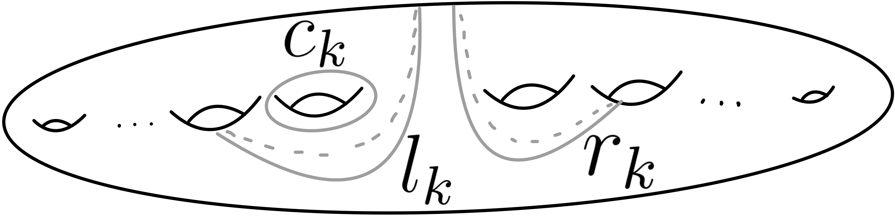
Left and right curves

Non-symmetrical down curve nd.

Non-symmetrical left and right curves nl, nr.
We set
Remark 4.1.
Note that the subcomplex
4.2 Proving the rigidity of
F
R
The first step is to check that the locally injective simplicial map
Lemma 4.2.
Let S be a finite-type surface, let
Then
Proof.
We will proceed by contradiction. Suppose that the curves
If

There can be no arc
Now, we prove that ϕ preserves non-adjacency rel to P.
Lemma 4.3.
Let S be a closed surface of genus
Proof.
Assume that for two curves
By means of the method above, we are only left to find appropriate subsets
If
It is straightforward to check that these subsets satisfy the conditions of Lemma 4.2,
and so
If
If
If
If
This concludes the proof. ∎
Using the previous result, we prove that ϕ preserves adjacency rel to P.
Lemma 4.4.
Let S be a closed surface of genus
Proof.
Take
We now determine the curves adjacent to
and the curves adjacent to
In the same style, we can argue inductively to determine the adjacency of each curve in
As a corollary, we obtain that ϕ preserves the topological type of P.
Corollary 4.5.
Let S be a finite-type surface and let
Proof.
We construct a homeomorphism h inductively by gluing abstract pairs of pants.
Consider the pairs of pants
The next three lemmas prove that
Lemma 4.6.
The subcomplex
Proof.
Let
Seeking a contradiction to case (i), we assume
To prove case (ii), the same argument works. ∎
Remark 4.7.
Notice that from the previous lemma we actually know that
Lemma 4.8.
The subcomplex
Proof.
Let
So, we can rename
With the previous simplification, the proof boils down to check that

Torus
By Lemma 4.6,
To finish, note that
Lemma 4.9.
The subcomplex
Proof.
Let
Now, we start by proving the cases
To prove that

Pair of pants bounded by
It is left to prove the cases

Pair of pants
Before proving that
To finish the proof, we check that
So far we have seen that the map
Lemma 4.10.
Let S be a closed surface of genus
Proof.
By Corollary 4.5, there exists
First, we find a homeomorphism that agrees with ϕ on

Torus
The same argument with minor changes yield homeomorphisms that agree with ϕ on every
To finish the proof, we are going to check that ϕ is fixing
Notice that
To prove that ϕ fixes U, consider
To prove that ϕ fixes D, consider
To prove that ϕ fixes L, consider the curve
Summarizing, we have proven that there exists a mapping class
This concludes the proof. ∎
To finish the proof of Theorem 1.1, we need to check that we can take ϕ to agree with a homeomorphism on
Proof of Theorem 1.1 for closed surfaces.
Let
Consider
We continue by proving that ϕ fixes nl. Note that
So far, we have found a composition of mapping classes
To prove the uniqueness of the inducing mapping class, suppose that
5 Finite rigid exhaustion for closed surfaces
In this section, we prove that, for any closed surface S of genus
such that each
The strategy to produce an exhaustion is to first extend
The plan of the proof is summarized in the following lemma (cf. [2, Lemma 3.13]).
Lemma 5.1.
Let S be a finite-type surface, let
satisfy that
Proof.
First, notice that if
We will now check that
for every
we deduce
For
for some
To produce the finite rigid exhaustion of
5.1 Enlarging the finite rigid set
Let
Note that the set
Figure 7
Curves in A for a closed surface.
Curves in

Curves in
We proceed to define
Lemma 5.2.
Let S be a closed surface of genus
Remark 5.3.
In the argument below, we sometimes abuse notation using
Proof.
Take a locally injective simplicial map
First, we check that ϕ fixes
By an obvious modification of the above argument, we check that
for
It is left to check that
Notice that the only curve in Q distinct from curves in
We have proven that if ϕ fixes
We define
5.2 Constructing the exhaustion for closed surfaces
Let ι be the back-front orientation reversing involution and let
are known as the Humphries generators, which are known to generate the group of orientation preserving mapping classes
Lemma 5.4.
Let
Proof.
First, we prove it for
Since
Proving that
Recall that
where
Note that
which is equivalent to
since
It can be directly checked that equation (5.1) is satisfied if and only if
The rest of the cases
If
If
If
If
If
If
To finish the proof, we need to consider the case
Proof of Theorem 1.2 for closed surfaces.
Let S be a closed surface of genus
6 Finite rigid sets for punctured surfaces
Let
6.1 Constructing the finite rigid set
We start by naming some curves in the punctured surface S.
Consider the closed surface
After this, we define the top of the surface, i.e.,
The set P is no longer a pants decomposition in S; to fix this we add some curves. First, rename
In this setting, we also define the back-front (orientation reversing) involution as the unique non-trivial element
Let
Let
Lastly, we define the set
Note that the set
Curves in

Pants decomposition P for

Curves in C for

Up and down curves

Curves

Curves

Curves
The finite rigid set
Remark 6.1.
Note that the subcomplex
The following lemmas prove the finite rigidity of
Lemma 6.2.
Let S be a punctured surface of genus
Proof.
First, notice that we can extend Lemma 4.3 to the case of punctured surfaces, and the proof works with minor changes.
Lemma 4.4 can also be extended to punctured surfaces. The proof for once punctured surfaces is similar to the closed case. Here we prove it for surfaces with
Using Remark 2.1, it is straightforward to deduce that the curve
Once we know that ϕ preserves adjacency rel to P, we can use Corollary 4.5 to produce a mapping class
The next lemma proves that we may choose
Lemma 6.3.
Let S be a punctured surface of genus
Proof.
The idea is to progressively detect intersections between curves and, by composing with Dehn twists along P, construct a mapping class that coincides with ϕ on
First, by Lemma 6.2, there exists
Next, using the same arguments as in Lemmas 4.6, 4.8 and 4.9, we detect the following intersections:
Intersections of curves in
Intersections of curves in Pl with curves in P.
Intersections of curves in Pr with curves in P.
Notice that we can now use the proof of Lemma 4.10 to produce a mapping class that coincides with ϕ on the curves of U, D and
It follows that ϕ fixes the curves in Pl. To see this, note that
Now, note that ϕ detects the following intersections:
Curves in
Curves in
For instance, consider
Using the above intersections and fixed curves, we now focus on finding a homeomorphism that agrees with ϕ on the curves in
Observe that
For
It is now easy (but lengthy) to check that the curves in
are fixed by ϕ. Thus, we have found a mapping class
We have essentially completed the proof of Theorem 1.1.
7 Finite rigid exhaustion for punctured surface
Let S be a punctured surface of genus
The strategy to construct the exhaustion is the same as in the closed case (see Section 5). First, we are going to enlarge the finite rigid set
7.1 Enlarging the finite rigid set
First, we enlarge
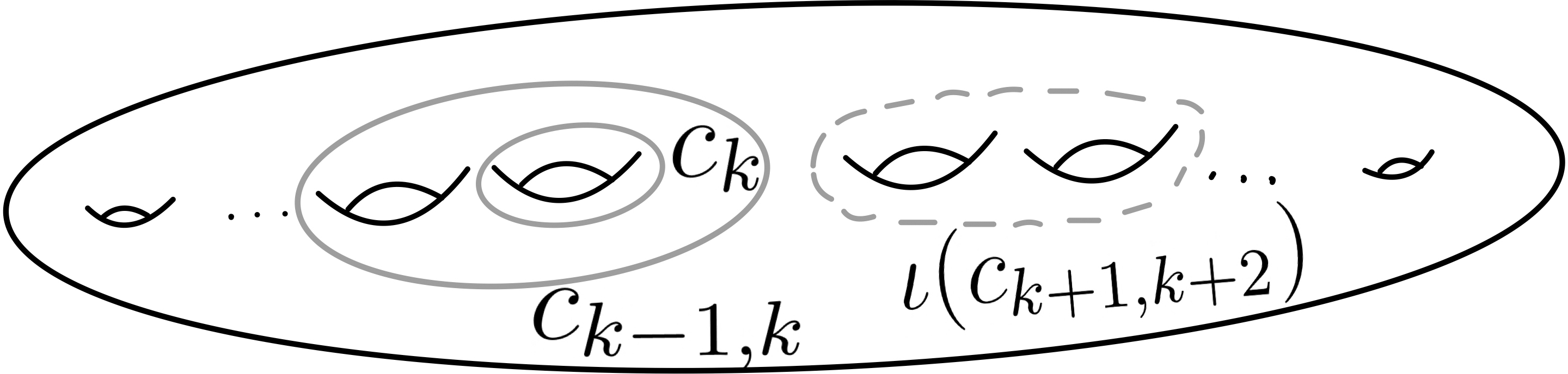
Consider the set of curves
We define the set of curves
We set

Curves
Lemma 7.1.
The set
Proof.
Let
First, we prove that
To prove that
To finish the proof, we must show that
that is not
We define
7.2 Constructing the exhaustion for punctured surfaces
The goal of this section is to construct an exhaustion of
Let ι be the back-front orientation reversing involution. Consider the usual Humphries generators
and the half twists
where
generates
Lemma 7.2.
For every
the set
Proof.
The proof is analogous to the closed case (see Lemma 5.4) and works directly for
Recall that, given
Thus, the proof is a matter of checking that
For
we can consider the curves
The last case to prove is
We now complete the proof of Theorem 1.2.
Funding source: Agencia Estatal de Investigación
Award Identifier / Grant number: CEX2019-000904-S
Funding statement: The author acknowledges financial support from grant CEX2019-000904-S funded by MCIN/AEI/ 10.13039/501100011033.
Acknowledgements
The author would like to thank his supervisor Javier Aramayona for suggesting the problem and for the guidance provided.
References
[1] J. Aramayona and C. J. Leininger, Finite rigid sets in curve complexes, J. Topol. Anal. 5 (2013), no. 2, 183–203. 10.1142/S1793525313500076Search in Google Scholar
[2] J. Aramayona and C. J. Leininger, Exhausting curve complexes by finite rigid sets, Pacific J. Math. 282 (2016), no. 2, 257–283. 10.2140/pjm.2016.282.257Search in Google Scholar
[3] T. E. Brendle and D. Margalit, Commensurations of the Johnson kernel, Geom. Topol. 8 (2004), 1361–1384. 10.2140/gt.2004.8.1361Search in Google Scholar
[4] B. Farb and D. Margalit, A Primer on Mapping Class Groups, Princeton Math. Ser. 49, Princeton University, Princeton, 2012. 10.1515/9781400839049Search in Google Scholar
[5] J. Hernández Hernández, C. J. Leininger and R. Maungchang, Finite rigid subgraphs of pants graphs, Geom. Dedicata 212 (2021), 205–223. 10.1007/s10711-020-00555-1Search in Google Scholar
[6] J. Huang and B. Tshishiku, Finite rigid sets and the separating curve complex, Topology Appl. 312 (2022), Paper No. 108078. 10.1016/j.topol.2022.108078Search in Google Scholar
[7] S. P. Humphries, Generators for the mapping class group, Topology of Low-Dimensional Manifolds (Chelwood Gate 1977), Lecture Notes in Math. 722, Springer, Berlin (1979), 44–47. 10.1007/BFb0063188Search in Google Scholar
[8] E. Irmak, Complexes of nonseparating curves and mapping class groups, Michigan Math. J. 54 (2006), no. 1, 81–110. 10.1307/mmj/1144437439Search in Google Scholar
[9] E. Irmak, Edge-preserving maps of the nonseparating curve graphs, curve graphs and rectangle preserving maps of the Hatcher–Thurston graphs, J. Knot Theory Ramifications 29 (2020), no. 11, Article ID 2050078. 10.1142/S0218216520500789Search in Google Scholar
[10] E. Irmak and M. Korkmaz, Automorphisms of the Hatcher–Thurston complex, Israel J. Math. 162 (2007), 183–196. 10.1007/s11856-007-0094-7Search in Google Scholar
[11] E. Irmak and J. D. McCarthy, Injective simplicial maps of the arc complex, Turkish J. Math. 34 (2010), no. 3, 339–354. 10.3906/mat-0812-16Search in Google Scholar
[12] N. V. Ivanov, Automorphism of complexes of curves and of Teichmüller spaces, Int. Math. Res. Not. IMRN 1997 (1997), no. 14, 651–666. 10.1155/S1073792897000433Search in Google Scholar
[13] Y. Kida, Automorphisms of the Torelli complex and the complex of separating curves, J. Math. Soc. Japan 63 (2011), no. 2, 363–417. 10.2969/jmsj/06320363Search in Google Scholar
[14] D. Margalit, Automorphisms of the pants complex, Duke Math. J. 121 (2004), no. 3, 457–479. 10.1215/S0012-7094-04-12133-5Search in Google Scholar
[15] R. Maungchang, Finite rigid subgraphs of the pants graphs of punctured spheres, Topology Appl. 237 (2018), 37–52. 10.1016/j.topol.2018.01.009Search in Google Scholar
[16] J. McCarthy and A. Papadopoulos, Simplicial actions of mapping class groups, Handbook of Teichmüller Theory, Volume III, European Mathematical Society, Zürich (2012), 297–423. 10.4171/103-1/6Search in Google Scholar
[17] E. Shinkle, Finite rigid sets in arc complexes, Algebr. Geom. Topol. 20 (2020), no. 6, 3127–3145. 10.2140/agt.2020.20.3127Search in Google Scholar
[18] E. Shinkle, Finite rigid sets in flip graphs, Trans. Amer. Math. Soc. 375 (2022), no. 2, 847–872. 10.1090/tran/8407Search in Google Scholar
© 2024 Walter de Gruyter GmbH, Berlin/Boston
This work is licensed under the Creative Commons Attribution 4.0 International License.
Articles in the same Issue
- Frontmatter
- The C*-algebra of the Boidol group
- Profinite genus of fundamental groups of compact flat manifolds with the cyclic holonomy group of square-free order
- Positive rigs
- Torus bundles over lens spaces
- Topological amenability of semihypergroups
- On projections of the tails of a power
- Li–Yorke chaos for composition operators on Orlicz spaces
- A note on the post quantum-Sheffer polynomial sequences
- Finite rigid sets of the non-separating curve complex
- Building planar polygon spaces from the projective braid arrangement
- Octonionic monogenic and slice monogenic Hardy and Bergman spaces
- Transcendence on algebraic groups
- An explicit version of Bombieri’s log-free density estimate and Sárközy’s theorem for shifted primes
- The ideal structure of partial skew groupoid rings with applications to topological dynamics and ultragraph algebras
- Joint distribution of the cokernels of random p-adic matrices II