Development of a new aerofoil profile with a high lift-to-drag ratio for wind turbines using a low fidelity accurate optimization flow solver
-
Moutaz Elgammi

 ,
Aljonid Aokaly
,
Aljonid Aokaly

Abstract
A significant amount of work is performed on various aerofoil profiles to improve their characteristics for wind turbine applications. The main purpose is to increase the power output of wind turbines by increasing the lift-to-drag ratio of the aerofoil blade sections. However, most of the developed aerofoil profiles work well only at their design angles of attack and for low Reynolds numbers with a very dramatic stall that could significantly influence the characteristics of the aerofoil profiles and the performance of wind turbines. The present paper is conducted to develop a new aerofoil profile with more gradual stall characteristics that works efficiently for different operational conditions (clean and rough working conditions) similar to those encountered by wind turbines in the free environment. The new aerofoil profile was developed based on a combination between experimental Box–Behnken design and XFOIL code, measurements, and 2D simulation conducted by computational fluid dynamics (CFD) method. The established aerofoil can be used for wind turbine blades because it gives high lift-to-drag-ratios with very smooth and gradual stall characteristics even under very rough operating conditions.
Introduction
Owing to the increase in population and urbanization in developing countries, electric power requirements have raised significantly all over the world. The dependence of power generation on depleting fossil fuels and natural gas resources side by side with ever-growing environmental concerns demands exploration of renewable and environment-friendly power generation methods (WEC 2013). Renewable energy methods involving hydroelectric, solar power conversion, and wind power extraction are being actively carried out worldwide to help meet the ever-growing electric power requirements (Chakraborty and Razzak 2014).
The aerodynamic design of the wind turbine blades is one of the principal problems of the wind industry, which has an outstanding influence on the output of maximum power for wind turbines. The blade of the wind turbine consists of one or more different aerofoil profiles along the blade. The blade can be divided into three main areas: root region, middle region, and tip region. The root region of the blade is built up from aerofoil profiles with a high thickness to chord ratio. Thick aerofoil profiles usually have a lower lift to drag ratio, and therefore, special consideration is required to increase the lift force of the aerofoil for more efficient wind turbine designs (Fuglsang and Bak 2004; Rooij and Timmer 2003). Researches (Anaya-Lara et al. 2011; Schubel and Crossley 2012) stated that wind turbines require a special aerofoil design to increase their power outputs at various flow conditions. In fact, the sudden stall presented on an aerofoil section can also significantly impact on the power output of wind turbines. Therefore, the “gentle stall” is needed for wind turbine aerofoil to avoid such significant losses of energy harvesting (Ahmed 2012).
A great attempt has been done to develop wind turbine technology. National Advisory Committee for Aeronautics (NACA 1949) designed four and five-digit aerofoil series for early modern wind turbines (Hau 2006). These digits classify the geometric profile of the aerofoil as follows: first digit indicates the maximum camber to the chord ratio, second digit refers to the location of the camber in the 10th of the chord, while third and fourth digits together are the percentage maximum thickness to chord ratio (Abbott and Doenhoff 1949). Alternatively, many other energy organizations and universities established different aerofoil profiles for the wind turbine industry such as the Delft University (Timmer and van Rooij 2003), LS, SERI-NREL, and FFA (Burton 2011) and RISO (Fuglsang and Bak 2004).
China has become in the lead throughout the world in the field of wind power generation. The CAS-W1 aerofoil families were designed by the Chinese Academy of Sciences. These aerofoil profiles have thicknesses of 15–25%. (Xu 2010) showed that the CAS-W1-250 aerofoil has a maximum thickness of 25% and a TE thickness of 0.6%. At Re = 3106, the aerofoil has very good aerodynamic characteristics with CL,max of 1.7 at 15° in clean conditions and 1.66 with LE roughness at the same conditions. At the design angle of attack of 6°, the L/D is equal to 157.6. (Chandrala et al. 2013) selected a single NACA 0018 aerofoil to make a rotor blade. The CFD analysis was carried out using ANSYS CFX software at different angles of attack at a constant wind speed of 32 m/s. The velocity and pressure distributions at various blade angles of attack were determined and they were found to be in good agreement with measurements. The optimal angle of attack at a wind speed of 32 m/s is 10°.
The aerofoil design process is essential in engineering design. It can be categorized into three methods: direct design, inverse design and optimization. In the direct design method (Xu 2010), the specifications of aerofoil design geometry is dictated by the outcome analysis, inferred from wind-tunnel or flight tests. The inverse design method (Vicini and Quagliarella 1997; Petrucci and Filho 2007), determines an aerofoil shape iteratively based on the target surface pressure distribution. There are various optimization methods which are developed over time for aerofoil design such as the conjugate gradient method (XiaoPing et al. 2015), Aquasi-Newton optimization method (Kennelly 1983), the gradient search optimization approach (Zhang et al. 2021), stochastic optimization methods (genetic algorithms (Quagliarella and Cioppa 1995) and simulated annealing (Liu 2005)). A combination between different optimization methods is also available. (Shahrokhi and Jahangirian 2007) applied an optimization approach to the shape of an aerofoil. Two parameterization methods were applied based on the flow characteristics of transonic viscous flow. A Genetic Algorithm was used as the optimization method and the shape of a viscous transonic aerofoil was optimized at high Reynolds number turbulent flow conditions. (Herrmann and Bangga 2019) improved the aerodynamic performance of the thick DU 00-W-401 aerofoil using a genetic algorithm approach for large wind turbine rotors under fixed and free transition conditions. It was found that the aerodynamic performance under fixed conditions was significantly improved, while for the free transition test, the results were slightly improved. (Tesfahunegn et al. 2015) presented a space mapping algorithm to optimize the aerofoil shape considering adjoint sensitivities. The design process showed lower computational costs compared with the high fidelity CFD simulation methods. (Sanaye and Hassanzadeh 2014) carried out a multi-objective optimization approach to maximize the aerofoil lift-to-drag ratio. A genetic algorithm method along with ‘Fuzzy Bellman-Zadeh’ decision-making method was applied as an optimization process. An average increase of 26% in the lift-to-drag ratio of the developed S822 aerofoil was obtained compared to the typical S822 aerofoil.
The main objective of this paper is to design a new aerofoil profile with a high lift-to-drag ratio aerofoil, but also with much softer stall and stable characteristics over various operating conditions that match those experienced by horizontal axis wind turbines (at Reynolds number of 1 × 10⁶). To achieve this, the boundary layer on the upper and lower surfaces of the aerofoil has been investigated, particularly the transitional area and its influence on the aerofoil characteristics. In this paper, the following aspects will be addressed:
The relationship between the location of the transitional area and the lift and drag force coefficients for different operating conditions.
The impact of the aerofoil geometry (leading edge radius, thickness, and curvature) on the stall characteristics, the lift and drag force coefficients and the transitional area at different angles of attack at Reynolds number of 1 × 10⁶.
The influence of the turbulence on the stall behaviour of the new aerofoil characteristics using CFD and measurements.
The influence of the combined impact of very high turbulent intensity and surface rough on the performance of the aerofoil at Reynolds number of 1 × 10⁶.
Methodology
XFOIL code
This code is an open source code developed by Mark Drela at the Massachusetts Institute of Technology in 1986 (Drela 1989). It is an interactive program for the design and analysis of subsonic isolated aerofoil profiles based on a coupled panel method/boundary layer method. It also incorporates inverse design theory, allowing an aerofoil to be constructed from a given pressure distribution. Therefore, it is possible to test and modify a large number of aerofoil profiles accordingly.
The inviscid formulation of XFOIL code
A simple linear-vorticity stream function panel method is used as an inviscid formulation. A two-dimensional inviscid flow field is constructed by the superposition of free stream flow, a vortex sheet of strength γ and a source sheet of strength σ on the aerofoil surface as shown in Figure 1. The trailing edge thickness is modeled by a source panel. The stream function is defined by:
where r is the magnitude of the vector between the path coordinate S and field points x, y and the vector’s angle θ.
Modelling the aerofoil and its wake by panel method along with vorticity and source distributions
Details of the trailing edge

(a) Modelling the aerofoil and its wake by panel method along with vorticity and source distributions, and (b) details of the trailing edge. Figure is adapted from (Drela 1989).
The equations are closed by applying an explicit Kutta condition, in which the source sheet
The viscous formulation of XFOIL code
A two-equation integral boundary layer formulation is used to calculate the boundary layer and wake. Using the surface transpiration model, the viscous solution has an interaction with the incompressible potential. Transpiration is a method in which extra nonphysical normal flows are created on an aerofoil surface to form a new streamline pattern; this surface streamlines no longer follow the aerofoil surface under inviscid flow (Yiu and Stow 1994). Therefore it enables calculating regions of limited separated flow. Whereas the panel methods are used to calculate the total velocity on all locations of the aerofoil surface, its wake, the aerofoils surface vorticity distribution, and the equivalent viscous source distribution. The standard compressible integral momentum and kinetic shape parameter equations are given as follows:
where ξ is the streamwise coordinate. More details can be found in (Ferreira 2002; Garcia 2011; Yiu and Stow 1994).
In the XFOIL code, the transition location for natural transition is predicted by an eN method caused by linear instability growth (Tollmien–Schlichting (TS) waves). The amplification of the waves is described by eN, in which N is the transition amplification factor. Transition in the boundary layer occurs when eN reaches
Aerofoil optimization method
Unlike traditional optimisation approaches which are discussed in the introduction section, the current approach uses the experimental Box–Behnken design (Montgomery 2001; Souza et al. 2005). This method is rotatable second-order designs based on chosen input design variables. The levels of the Box–Behnken design are arranged to increase the design points with a rate similar to the polynomial coefficients. Although this method is mainly applied for modelling many engineering problems (Annadurai et al. 2004; Rana et al. 2004), design (Montgomery 2001; Souza et al. 2005), depending on sets of experimental data, they are utilized in the present work to perform aerofoil shape optimization based on the XFOIL code as an alternative to the measurements. To the author’s knowledge, these techniques have not been applied before to optimize aerofoil profiles. The proposed aerofoil optimization scheme utilized in this work is explained in detail as follows:
Shape function: The present design approach starts with a given shape function for the desired aerofoil. The selected aerofoil shape function is the 4-digit NACA aerofoil family. More than 50 aerofoil profiles of the 4-digit NACA aerofoil family were compared to choose the best profiles with the required conditions. The boundary layers on the upper and lower surfaces of the selected aerofoil profiles were then analysed by the XFOIL code, particularly the transitional area and its impact on the aerofoil characteristics. Understanding the latter influence will allow the designer to improve the aerofoil performance as required. It should be noted that the shape functions of the other aerofoil families can also be used.
Design variables: The focus in the current work is on the leading-edge radius, maximum thickness and camber, which are considered as design variables to optimize the aerofoil for high aerodynamic performance.
Object/target: In the present approach, the target is to maximize the lift-to-drag ratio for either smooth or rough conditions or even a trade-off between smooth and rough conditions. The influence of turbulent intensity and roughness are considered in the current optimization approach by the use of NCrit in the XFOIL code. An NCrit value of 4.25 translates to a turbulent intensity (I) of 0.50%, while an NCrit value of 3.25 is equal to a turbulent intensity (I) of 0.75%, which both corresponds to a reasonably turbulent environment. An NCrit value of nine corresponds to a turbulent intensity (I) of 0.07%, which is appropriate for clean conditions.
Design constraints: The chosen three design variables (leading-edge radius, maximum thickness and maximum camber as a function the aerofoil chord (c)) for the Box–Behnken design used in this study are given in Table 1.
Variable levels for the Box–Behnken design.
| Variable | Symbol | Coded variable level | ||
|---|---|---|---|---|
| Low | Centre | High | ||
| −1 | 0 | +1 | ||
| Maximum camber | x 1 | 0.02c | 0.04c | 0.06c |
| Maximum thickness | x 2 | 0.12c | 0.15c | 0.18c |
| Leading-edge radius | x 3 | 0.0110c | 0.0159c | 0.0216c |
For these three design variables (see Table 1), a total of 15 test runs is performed. For each new generated configuration (leading-edge radius, maximum thickness and maximum camber), a new aerofoil geometry is created by a Matlab code. The maximum lift-to-drag ratio of each new aerofoil is then determined by the XFOIL code at Mach number of 0.2 and Reynolds number of 1 × 10⁶ as illustrated in Table 2. It should be noted that in the experimental Box–Behnken design, measurements are performed. However, is not possible to manufacture and analyse each individual new aerofoil. Therefore, it is assumed that the XFOIL code could replace the wind tunnel measurements in this study.
Objective function: The following quadratic model is developed based on the data set in Step 4:
where y represents the maximum lift-to-drag ratio, β0 is the model constant, x1, x2, and x3 are the design constrains/variables, β1,β2, and β3 are linear coefficients, β12,β13, and β23 are cross product coefficients, and β11,β22, and β33 are the quadratic coefficients. These coefficients are estimated from the generated 15 test runs explained in Step 4 using the least square method.
Constrained nonlinear optimization function (using fmincon solver in Matlab) is applied to find a constrained minimum of a scalar function (Eq. (5)) of the design constrains created in Step 4. The maximum lift-to-drag ratio and the corresponding optimum design variables that maximize the lift-to-drag ratio are determined and the new optimized aerofoil profile is finally established.
Box–Behnken design with real/coded values for chosen three design variables.
| Run no. | Real and coded level of variables | XFOIL prediction max.(CL/CD) | |||||
|---|---|---|---|---|---|---|---|
| x 1 | x 2 | x 3 | |||||
| Real | Coded | Real | Coded | Real | Coded | ||
| 1 | 0.02c | −1 | 0.18c | 1 | 0.0159c | 0 | 52.9 |
| 2 | 0.06c | 1 | 0.12c | −1 | 0.0159c | 0 | 69.1 |
| 3 | 0.04c | 0 | 0.12c | −1 | 0.0216c | 1 | 71.9 |
| 4 | 0.06c | 1 | 0.15c | 0 | 0.0110c | −1 | 57.3 |
| 5 | 0.02c | −1 | 0.15c | 0 | 0.0110c | −1 | 63.7 |
| 6 | 0.02c | −1 | 0.15c | 0 | 0.0216c | 1 | 62.9 |
| 7 | 0.06c | 1 | 0.18c | 1 | 0.0159c | 0 | 45.8 |
| 8 | 0.02c | −1 | 0.12c | −1 | 0.0159c | 0 | 69.9 |
| 9 | 0.04c | 0 | 0.15c | 0 | 0.0159c | 0 | 61.4 |
| 10 | 0.06c | 1 | 0.15c | 0 | 0.0216c | 1 | 57.3 |
| 11 | 0.04c | 0 | 0.15c | 0 | 0.0159c | 0 | 61.4 |
| 12 | 0.04c | 0 | 0.18c | 1 | 0.0110c | −1 | 50.0 |
| 13 | 0.04c | 0 | 0.12c | −1 | 0.0110c | −1 | 72.3 |
| 14 | 0.04c | 0 | 0.18c | 1 | 0.0216c | 1 | 49.8 |
| 15 | 0.04c | 0 | 0.15c | 0 | 0.0159c | 0 | 61.4 |
The total computation cost of the proposed optimization approach takes less than 3 min on a personal computer with Intel Core, I7, 4700MQ CPU @ 2.4 GHz and RAM of 8 GB. This is considerably small time compared to most of the traditional optimization methods in the literature.
Computation fluid dynamics (CFD) method
It is important to ensure that the stall characteristics of the developed aerofoil profile are stable and gradual without a sudden drop in the lift force and a sudden increase in the drag force. Therefore, the flow around the new aerofoil was analysed by an open source CFD code, OpenFOAM® (Greensheilds 2015). In OpenFoam, the standard (k–ω) model is mainly adopted from the work of Wilcox (2008), which uses modifications for the effects of low-Reynolds number, compressibility and shear flow spreading. The standard (k–ω) model is an empirical model which is based on model transport equations for modelling the turbulent kinetic energy (k) and the specific dissipation rate (ω). Both the k and ω equations have been modified over time to improve their accuracy for predicting free shear flows. The general forms of the turbulent kinetic energy (k) and the specific dissipation rate (ω) can be derived from the below transport equations:
where Gk is the generation of turbulent kinetic energy due to mean velocity gradients, Gω is the generation of ω, Γk and Γω are the effective diffusivity of k and ω respectively, Yk and Yω are the dissipation of k and ω due to turbulence, and Sk and Sω are user-defined source terms.
The domain and mesh are presented in Figures 2 and 3. Higher grid density was made close to the aerofoil wall to ensure modelling the boundary layer with sufficient accuracy. For the computational domain in Figure 2, several grids/meshes have been applied using quadrilateral cells as illustrated in Tables 3 and 4. Each grid was made very dense (with a starting cell height of 1e-4) near the aerofoil surface to capture the pressure gradient at the boundary layer with sufficient accuracy. This is important because the adverse pressure gradient causes the flow separation. In the far-field area of the computational domain, the resolution of the mesh was made a standard grid due to the fact that the flow gradients approach zero away from the aerofoil.

The domain and mesh used for simulation of the flow past aerofoil.

Mesh of the computational domain and around NACA 2415 aerofoil by using the structured grid.
Comparisons of the lift and drag force coefficients between experiment (Abbott and Von Doenhoff 2012) and CFD results (NACA2415 aerofoil) for different meshes at 8° angle of attack at Re = 3 × 10⁶.
| Grids | Number of cells | Average y+ | Experiment | CFD | Error (%) | |||
|---|---|---|---|---|---|---|---|---|
| C L | C D | C L | C D | ε CL | ε CD | |||
| Grid 1 | 6200 | 46 | 1.12 | 0.012 | 0.95 | 0.020 | 15.17 | 66.66 |
| Grid 2 | 10,080 | 32 | 1.12 | 0.012 | 1.03 | 0.015 | 8.03 | 25 |
| Grid 3 | 219,600 | 2.45 | 1.12 | 0.012 | 1.12 | 0.012 | 0 | 0 |
| Grid 4 | 259,160 | 0.55 | 1.12 | 0.012 | 1.12 | 0.012 | 0 | 0 |
Comparisons of the lift and drag force coefficients between experiment (Abbott and Von Doenhoff 2012) and CFD results (NACA2415 aerofoil) for different meshes at 15° angle of attack at attack at Re = 3 × 10⁶.
| Grids | Number of cells | Average y+ | Experiment | CFD | Error (%) | |||
|---|---|---|---|---|---|---|---|---|
| C L | C D | C L | C D | ε CL | ε CD | |||
| Grid 1 | 6200 | 46 | 1.37 | 0.021 | 1.05 | 0.015 | 23.35 | 28.57 |
| Grid 2 | 10,080 | 32 | 1.37 | 0.021 | 1.29 | 0.019 | 5.83 | 9.52 |
| Grid 3 | 219,600 | 2.45 | 1.37 | 0.021 | 1.34 | 0.022 | 2.18 | 4.76 |
| Grid 4 | 259,160 | 0.55 | 1.37 | 0.021 | 1.345 | 0.020 | 1.82 | 4.76 |
In this approach conservation of mass and momentum equations are discretized according to the standard Gaussian finite-volume integration. These equations are integrated over the volume, whereas the convective and diffusive terms are converted to surface integral with the use of Gauss’ divergence theorem. The volume and surface integrals are approximated by a second-order accurate midpoint scheme. In the latter approach, a linear interpolation is applied to determine the unknown values on the cell faces. Gaussian integration is applied by taking the sum of the values on the cell faces.
Since the turbulent flow field is described by the (k-ω) model, it is necessary to implement a very small time step according to the grid refinement. Therefore, the courant number (Co = U∞Δt/Δx), where Δx is the average distance between two cell centroids on the aerofoil wall, and Δt is the time step, was selected to be ≤1 to ensures that fluid particles move from one cell to another within one time step with stable and converged solutions, and optimal error damping properties. The average wall y+ distributions over the NACA2415 aerofoil at α = 8ο and 15ο at Re = 3 × 10⁶ are also presented in Tables 3 and 4. From Tables 3 and 4, it is obvious that the Grids 1 and 2 give unacceptable error compared to measurements as determined by Eq. (8), while the Grids 3 and 4 give satisfied results. The wall y+ distributions for Grids 3 and 4 are illustrated in Figure 4. In this paper, the y+ value was chosen to be less than unity for best accuracy as recommended by (Versteeg and Malalasekera 2007). Indeed, the required time step to simulate the flow on the mesh corresponding to Grid 4 is in the order of Δt = O(108) s. Therefore, all simulations were run using Grid 4 with models having a chord length of 1 m at Reynolds number of 1 × 10⁶, which corresponds to wind speed of 15 m/s respectively.

y+ distribution over the NACA2415 aerofoil at α = 8ο at Re = 3 × 10⁶.
Subsonic wind tunnel measurements
The experimental work is carried out in an open-ended subsonic wind tunnel located at the laboratory of the Omar Al-Mukhtar University, Derna, Libya. As seen from Figure 5, the subsonic wind tunnel is provided with a fan driven by a DC variable speed motor unit located downstream of the working section. The DC motor allows regulating the number of revolutions and therefore, the airspeed between 0 and 26 m/s. The air enters the test section through a designed contraction followed by an aluminum honeycomb flow straightener to create uniform flow and to break the large vortexes into small vortexes within the working test section. There are also inclined and multi-tube manometers to measure the air speed and static pressure in the wind tunnel. The dimensions of the wind tunnel are 2.98 m in length, 1.83 m in height, 0.8 m in width, and the test section is 30 × 30 ×45 cm. The turbulent intensity of the wind tunnel is around 0.07% at the maximum wind speed with a mean velocity variation of ±0.2 m/s.

Open-ended subsonic wind tunnel.
The subsonic wind tunnel is provided with a Pitot static tube (see Figure 6) to determine the air speed in the working test section. It has a 4 mm diameter stainless steel tube and of Prandtl design with a negligible correction up to yaw angles of at least 5°. The Pitot static tubes are connected to the multi-tube manometer by two tappings in order to measure the difference in pressure between the total and static tappings. The air speed in the working section is calculated by applying Bernoulli’s equation as follows:
where ρw is the density of air (kg/m3) and ΔP is the difference in pressure between the total and static tappings (N/m2). ΔP is measured using the tube manometer as follows:
where ρ is manometer fluid density (kg/m3), (water is used), g is gravitational constant (9.81 m/s2), and Δh is the true difference in manometer heights.

Pitot static tube.
The pressure distribution on the aerofoil can be expressed in terms of a dimensionless lift coefficient CP which, in turn, can be determined experimentally or numerically.
where pi is the surface pressure measured at location i on the surface, p∞ is the pressure in the free stream, ρ is air density, and U∞ is the free-stream velocity.
One important consideration to take into account in the subsonic wind tunnel is the presence of the solid tunnel boundaries which can cause variation in the flow field from the free-air flow. In order to avoid bounded air stream and inaccurate measurements, a set of corrections caused by the wind tunnel walls must be applied. In the current study, the phenomena of horizontal buoyancy, solid blockage, wake blockage, and stream curvature were all corrected according to the methods of (Allen 1944; Barlow, Rae, and Alan 1999).
Generating turbulence in wind tunnel experiments
Generation of turbulence in wind tunnels is important for studying wind turbine aerodynamics (Sicot et al. 2008). A turbulent inlet is usually generated using three families of grids: passive, active, and fractal. In this paper, the passive grid technique (Taylor 1935) is selected to generate wind tunnel turbulence. It should be noted that the designed turbulent inflow depends mainly on (1)- the width b of the bars, (2)- the mesh size M presenting the distance between the centerline of the bars, and (3)- the downstream distance

Schematic of the grid with bar b and mesh M size.
Empirical relations for turbulence characteristics (Roach 1987).
| Empirical expression | I = A(x/b) | I = AB(x/b) | L/b = C(x/b) |
|---|---|---|---|
| Constants | A=1.13 | B=0.89 | C=0.20 |
In this paper, it is desired to investigate the stall characteristics at turbulent intensities of 0.50 and 0.75%. Therefore, the passive grid was designed carefully to generate the required turbulent intensities at the inlet of the wind tunnel. Based on the optimal mesh size of M = L/8 and the test section length (L) of 45 cm, M is determined to be 0.0563 m. The width b of the bars, and the downstream distance
Geometry of the designed grids and the relevant turbulent intensities.
| Grid | x (m) | M (m) | b (m) | I (%) |
|---|---|---|---|---|
| 1 | 0.4 | 0.0563 | 0.005 | 5.1 |
| 2 | 0.8 | 0.0563 | 0.015 | 7.56 |
The passive grids in Table 6 were fabricated and placed at the inlet of the wind tunnel to generate the required turbulent intensities of 0.50 and 0.75% respectively. The wind speed was then measured at Reynolds number of 1 × 10⁶ over a period of 1 h. The measured standard deviations of the wind speed at Re = 1 × 10⁶ are 0.72 for I = 0.50% and 1.1 for I = 0.75%. These measured wind speeds will be used to analyse the impact of the turbulent intensity on the transitional area occurring on the upper surface of the aerofoil at different angles of attack and at Reynolds number of 1 × 10⁶.
The integral length scale (l) is determined by Taylor’s frozen eddy hypothesis as given by:
where the integral time scale (T) is calculated by:
The auto-correlation function of time (f(τ)) is
where u is the velocity fluctuation term and u’ is the standard deviation of the velocity fluctuation.
Results and discussion
This section presents the results conducted on the aerofoil profiles developed by the NACA (1949). NACA aerofoil profiles were compared to select the aerofoil profiles with the highest lift-to-drag ratios. From the comparisons, it was found that NACA 2415 has the highest lift-to-drag ratio of 103.702 at Re = 1 × 10⁶ as seen from Table 7, which depicts only results of some selected profiles for illustration of the comparisons. NACA 2415 has a maximum camber 2% of the chord length located at 40% chord from the leading edge with a maximum thickness 15% of the chord at 30% chord from the leading edge as shown in Figure 8. When the suitable aerofoil profile was selected, the baseline aerofoil (NACA 2415) was optimized to further increase the lift-to-drag ratio using the optimization approach described early. The optimized aerofoil profile has the following specifications: a maximum camber 5% of the chord length located at 40% chord from the leading edge with a maximum thickness 15% of the chord at 30% chord from the leading edge as illustrated in Figure 8.
Characteristics of the NACA series at Re = 1 × 10⁶.
| Aerofoil | α | CL | max (L/D) |
|---|---|---|---|
| NACA 2415 | 5.50 | 0.893 | 103.702 |
| NACA 2421 | 6.50 | 0.895 | 92.150 |
| NACA 2408 | 7.50 | 0.999 | 79.662 |
| NACA 2410 | 5.50 | 0.806 | 70.906 |
| NACA 4424 | 80 | 0.997 | 64.671 |

The geometry of the baseline aerofoil (NACA 2415), and the optimized aerofoil profiles.
Figure 9 illustrates comparisons for the lift force coefficients and lift-to-drag ratios with angles of attack between the baseline aerofoil (NACA 2415) and the optimized aerofoil shape profile at Re = 1 × 10⁶ for clean condition (NCrit = 9). In these results, the optimized aerofoil shape profile shows higher lift force coefficient and lift-to-drag ratio. With this improvement, the optimized aerofoil shape profile shows an average increase of more than 25% in the lift-to-drag ratio. These results show clearly that the curved surfaces generate higher lift forces than the flat or less curved surfaces. In Figure 9, it can also be seen that the decrease in the lift force coefficient at stall for the optimized aerofoil shape profile is more gradual and smooth compared with that for the baseline aerofoil (NACA 2415). In the attached flow regime, the lift force coefficient of the optimized aerofoil shape profile is higher than that for the baseline aerofoil (NACA 2415). The change from the attached flow regime to the post stall flow regime occurs earlier for the baseline aerofoil (NACA 2415) at static stall angle of attack of 150, while it occurs at 160 for the optimized aerofoil shape profile. This delay is mainly related to changing in the curvature of the aerofoil and the boundary layer flow separation.

Comparisons between characteristics of the baseline aerofoil (NACA 2415) and the optimized aerofoil shape profiles at Re = 1 × 10⁶ for clean condition (NCrit = 9).

Comparisons of the time averaged pressure coefficients between measurements with error bars and CFD results at Re = 1 × 10⁶.
Investigation of the stall characteristics: In the previous comparisons, it was depicted that the baseline aerofoil (NACA 2415) is the most suitable aerofoil profile. Therefore, the focus will be only on this profile in the following discussion. Table 8 presents the transitional area, determined by XFOIL code for clean conditions (NCrit = 9), on the upper surfaces of the baseline aerofoil (NACA 2415) and the optimized aerofoil shape profiles at different angles of attack at Re = 1 × 10⁶. From Table 8, it can be seen that the transitional point on the upper surface of the optimized aerofoil shape profile is delayed further downstream towards the trailing edge by increasing the angle of attack compared to the baseline aerofoil (NACA 2415), except at the deep stall flow regime (α = 200), where the transitional point comes closer to the leading edge of the optimized aerofoil shape profile. Table 8 shows that the optimized aerofoil has a larger laminar boundary layer region than the baseline aerofoil (NACA 2415), which benefits the lift force coefficient.
Transitional points on the aerofoil upper surface at Re = 1 × 10⁶ for clean condition.
| Aerofoil | 50 | 100 | 150 | 200 |
|---|---|---|---|---|
| Baseline aerofoil (NACA 2415) | 0.293 | 0.065 | 0.022 | 0.02 |
| Optimized aerofoil shape profile | 0.433 | 0.187 | 0.039 | 0.017 |
Impact of turbulence on the aerofoil characteristics: The strategy of the generation of turbulence in the wind tunnel was presented before (see Figure 7 and Table 6). A qualitative comparison of the CFD and experimental results of the surface pressure coefficient is illustrated in Figure 10. In these results, the surface pressure distributions at each turbulent intensity at Re = 1 × 10⁶ were measured over a period of 1 h. Each has been repeated 10 times for several days to have enough data points. In Figure 10, the error bars with measurements indicate around two standard deviations. In this comparison, the CFD results are in good agreement with measurements at all angles of attack and turbulent intensities.
Figure 11 shows velocity counters of the CFD results without turbulence for the optimized aerofoil shape profile at Reynolds number of 1 × 10⁶, while Figures 12 and 13 illustrate the same but for turbulent intensities of 0.50 and 0.75%. Form these results, it could be seen that the level of turbulence on the flow separation and the boundary layer momentum thickness has no significant influence in the attached flow regimes (at angles of attack of 5° and 10°) as shown in Figures 11(a, b)–13(a, b). Therefore, it can be concluded that the boundary layer momentum thickness and flow separation are constant and independent on pressure gradient in the attached flow regime for different turbulent intensities. However, different instability mechanisms are observed at near stall (α = 15°) and post stall (α = 20°) flow regimes for different turbulent intensities (see Figures 11(d, c)–13(d, c)). From these results, it is obvious that the structure of the separated shear layer and the transition criteria are slightly unstable for various turbulent intensities.
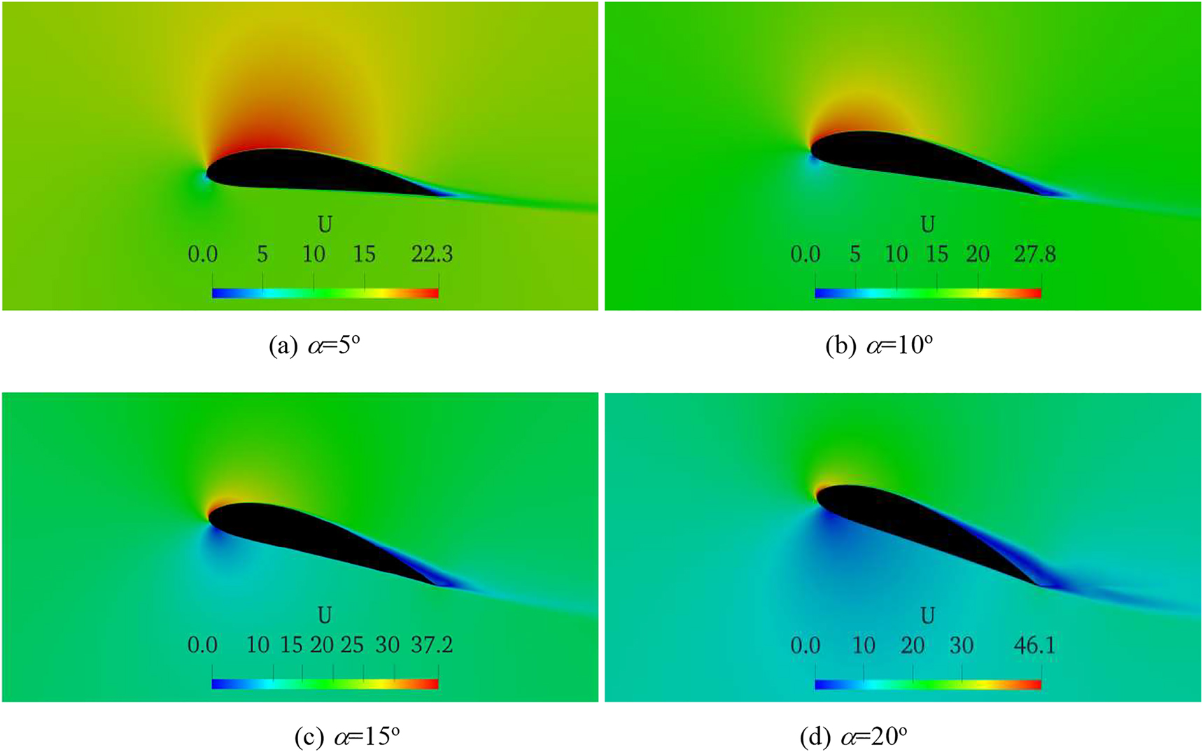
Contours of velocity magnitude for the optimized aerofoil shape profile at Re = 1 × 10⁶ (no turbulence).

Contours of velocity magnitude for the optimized aerofoil shape profile at Re = 1 × 10⁶ (I = 0.50%).

Contours of velocity magnitude for the optimized aerofoil shape profile at Re = 1 × 10⁶ (I = 0.75%).
To demonstrate the aerodynamic performance of the optimized aerofoil profile, a comparison with the baseline aerofoil (NACA 2415) is conducted at different turbulent intensities and also for smooth and rough surface flows at the same working conditions (Re = 1 × 10⁶, Ma = 0.2) as depicted in Figures 14 and 15. The roughness influence is important to investigate given that the loss of wind turbine power is due to the increased leading edge roughness (caused by insects, sand, salt, and rain over time) on the rotor blades, yielding to reduction in the aerodynamic performance. This impact is taken into account in the XFOIL code by forcing the transition of the boundary layer at 0.01 on the suction side and 0.1 on the pressure side. The maximum lift-to-drag ratio of the optimized aerofoil is 119.2 for the working condition of the smooth surface. This occurs at angle of attack of 6°, while for rough surface condition, the maximum lift-to-drag ratio of the optimized aerofoil is 57.3 at angle of attack of 6°. Although the optimized aerofoil profile is sensitive to the leading edge roughness condition, it still has a good stall characteristic. For the other range of angles of attack, the optimized aerofoil shows higher lift force coefficient and lift-to-drag ratio compared to the baseline aerofoil (NACA 2415) for both free and fixe transitions. It could be observed that the leading edge roughness does not influence on the lift force coefficient slope, but it leads to a reduction in the maximum lift force coefficient and an increase in the minimum drag force coefficient, and subsequently in the lift-to-drag ratio.

Lift force coefficients and lift-to-drag ratio for clean (free transition) and rough (fixed transition) operating conditions at Reynolds number of 1 × 10⁶.

Lift force coefficients and lift-to-drag ratio for different turbulent intensities at Reynolds number of 1 × 10⁶-free transition test case.
To analyse the influence of turbulent intensities, the XFOIL code is used with the following specifications: NCrit = 4.25 for turbulent intensity of 0.50%, and NCrit = 3.25 for turbulent intensity of 0.75% as shown in Figure 15. As it can be seen, when the level of turbulence is increased from 0.50 to 2.96%, the lift force coefficient is further reduced due to the increase in the turbulent kinetic energy in the flow separation zone of boundary layer and subsequently, the drag force coefficient is increased. At high turbulent intensity of 2.96%, the stall angle of attack occurs earlier than that at low turbulent intensities of 0.50 and 0.75%. This indicates that the transition of the boundary occurs close to the leading edge of the aerofoil under such rough conditions. The effect of the turbulent intensity also causes a small increase in the drag coefficient until the stall angle is reached, after which the drag force coefficient is increased suddenly. This is mainly due to the increase in the pressure drag force as a result of flow separation. In the attached flow regime, it can be observed that the slope of the lift force coefficients is almost the same for all turbulent intensities. When the static stall angle of attack is reached, the lift force coefficient decrease smoothly, indicating smooth and gradual stall characteristics.
An interesting feature, which has not been widely studied in the literature, is to investigate the combined influence of both turbulent intensity and surface roughness on the aerodynamic performance of the aerofoil. In the present work, this was achieved in the XFOIL code by setting a fixed transition to 0.01 and 0.1 on the upper and lower surfaces respectively and NCrit = 0.01 (I = 2.96%) as illustrated in Figure 16. For such rough working conditions, it is obvious that the optimized aerofoil performs better than the baseline aerofoil (NACA 2415) under the same flow conditions in terms of the lift force coefficient, lift-to-drag ratio, and stall characteristics. From these results, the combined impact of turbulent intensity and surface roughness yields to further drops in the lift force coefficient and the lift-to-drag ratio compared to those shown in Figures 14 and 15.

Lift force coefficients and lift-to-drag ratio for rough working conditions. In these results the transition is forced at 0.01 and 0.1 on the upper and lower surfaces respectively, while turbulent intensity of 2.96% corresponding to NCrit = 0.01 is considered.
Conclusions
The current paper was conducted to develop a new aerofoil profile with a high lift-to-drag ratio, smooth and gradual stall for wind turbine applications. The proposed optimization method is based on the use of the experimental Box–Behnken design and XFOIL code, computational fluid dynamics (CFD), and measurements to achieve the purpose. From this work, conclusions are drawn as follows:
A new aerofoil profile was developed from the geometric profile of the NACA 2415 aerofoil with the following specifications: a maximum camber of 5% chord located at 40% chord from the leading edge with a maximum thickness of 15% chord located at 30% chord from the leading edge.
The newly aerofoil profile provides more than 25% average increase in the lift-to-drag ratio compared to the baseline aerofoil (NACA 2415) under different working conditions. This shows a confidence in utilizing the present methodology for different aerofoils shapes of wind turbine blades.
The aerofoil thickness has a dramatic impact on the characteristics of the aerofoil. It was found that thicker aerofoil profiles increase the drag forces and decrease the lift forces, leading to a significant decrease in the lift-to-drag ratio. It is also recommended to consider the locations of the maximum thickness and camber of the aerofoil in the future to further improve the performance of the aerofoil profile using the methodology adopted in this paper.
To increase the lift-to-drag ratio, it is suggested that the transitional point on the upper surface of the aerofoil is delayed downstream from the leading edge using a suitable strategy.
High turbulent intensity and surface roughness increase the minimum drag force coefficient and reduce both the maximum lift force coefficient and the lift-to-drag ratio. Low turbulent intensity and smooth surface lead to a delay in the stall angle of attack and the flow separation point and thereby to an increase in the lift force coefficient.
The newly developed aerofoil has smooth and gradual stall characteristics at different operating conditions. The present study suggests the use of this aerofoil at middle span and blade tip sections of wind turbines since its gives good on-design and off-design aerodynamic performances. The blade root sections of a wind turbine are usually made of thick aerofoil profiles to resist the high stresses. Therefore, this needs to be investigated in the future using the strategy applied in this paper.
The main advantage of the proposed optimization method is that satisfactory results are obtained with minimum computational costs. This is a very important feature for the design or optimization of wind turbine blades using a low fidelity accurate flow solver.
-
Author contributions: All the authors have accepted responsibility for the entire content of this submitted manuscript and approved submission.
-
Research funding: None declared.
-
Conflict of interest statement: The authors declare no conflicts of interest regarding this article.
References
Abbott, I., and A. Doenhoff. 1949. Theory of Wind Sections. London: McGraw-Hill.Search in Google Scholar
Abbott, I. H., and A. E. Von Doenhoff. 2012. Theory of Wing Sections: Including a Summary of Airfoil Data. New York, USA: Courier Corporation.Search in Google Scholar
Ahmed, M. 2012. “Blade Sections for Wind Turbine and Tidal Current Turbine Applications–Current Status and Future Challenges.” International Journal of Energy Research 36 (7): 829–44, https://doi.org/10.1002/er.2912.Search in Google Scholar
Allen, J., and W. G. Vincenti. 1944. Wall Interference in a Two-Dimensional-Flow Wind Tunnel, with Consideration of the Effect of Compressibility. NACA-TR-782. National Advisory Committee for Aeronautics (NACA), Moffet Field, CA, USA.Search in Google Scholar
Anaya-Lara, O., N. Jenkins, J. Ekanayake, P. Cartwright, and M. Hughes. 2011. Wind Energy Generation: Modelling and Control. West Sussex, UK: John Wiley & Sons.Search in Google Scholar
Annadurai, G., S. S. Sung, and D. L. Lee. 2004. “Optimisation of Floc Characteristics for Treatment of Highly Turbid Water.” Separation Science and Technology 39: 19–42.10.1081/SS-120027399Search in Google Scholar
Barlow, J. B., W. H. Rae, and P. Alan. 1999. Low-Speed Wind Tunnel Testing, 3rd ed. New York: John Wiley & Sons.Search in Google Scholar
Burton, T. 2011. Wind Energy Handbook. Chichester: John Wiley & Sons.10.1002/9781119992714Search in Google Scholar
Chakraborty, S., and M. Razzak. 2014. “Design of a Transformer-Less Grid-Tie Inverter Using Dual-Stage Buck and BooConverters.” International Journal of Renewable Energy Resources 4 (1): 91–8.Search in Google Scholar
Chandrala, M., Choubey, A., and Gupta, B. 2013. “CFD Analysis of Horizontal Axis Wind Turbine Blade for Optimum Value of Power.” International Journal of Energy and Environment 4 (5): 825–34.Search in Google Scholar
Drela, M. 1989. “XFOIL: An Analysis and Design System for Low Reynolds Number Airfoils.” In Low Reynolds Number Aerodynamics. Lecture Notes in Engineering, Mueller, T. J. (ed), 54, 1–12. Berlin, Heidelberg: Springer.10.1007/978-3-642-84010-4_1Search in Google Scholar
Drela, M. M. I. S. E. S. 1998. Implementation of Modified Abu- Ghannam/Shaw Transition Criterion. MISES Code Documentation, MIT.Search in Google Scholar
Ferreira, C. 2002. “Implementation of Boundary Layer Suction in XFOIL and Application of Suction Powered by Solar Cells at High Performance Sailplanes.” Unpublished master’s thesis, Delft University of Technology.Search in Google Scholar
Fuglsang, P., and C. Bak. 2004. “Development of the Riso Wind Turbine Airfoils.” Wind Energy 7: 145–62, https://doi.org/10.1002/we.117.Search in Google Scholar
Garcia, N. R. 2011. “Unsteady Viscous-Inviscid Interaction Technique for Wind Turbine Airfoils.” Doctoral diss., Ph.D. thesis, Lyngby: Technical University of Denmark.Search in Google Scholar
Greensheilds, C. 2015. “Applications and Libraries.” In OpenFOAM: The Open Source CFD Toolbox (User Guide Version 3.0.1), 69–104. OpenFOAM Foundation Ltd.Search in Google Scholar
Hau, E. 2006. Wind Turbines, Fundamentals, Technologies, Application, Economics, 2nd ed. Berlin: Springer.10.1007/3-540-29284-5Search in Google Scholar
Herrmann, J., and G. Bangga. 2019. “Multi-objective Optimization of a Thick Blade Root Airfoil to Improve the Energy Production of Large Wind Turbines.” Journal of Renewable and Sustainable Energy 11: 043304, https://doi.org/10.1063/1.5070112.Search in Google Scholar
Kennelly, R. 1983. Improved Method for Transonic Airfoil Design by Optimization. AIAA paper 83-1864. Danvers: AIAA Applied Aerodynamics Conference.10.2514/6.1983-1864Search in Google Scholar
Laneville, A. 1973. Effects of Turbulence on Wind-Induced Vibrations of Bluff Cylinders. Vancouver: University of British Columbia.Search in Google Scholar
Liu, J.-L. 2005. “A Novel Taguchi-Simulated Annealing Method and its Application to Airfoil Design Optimization.” In Proceedings of the 17th AIAA Computational Fluid Dynamics Conference, Toronto, ON, Canada, 6–9 June 2005.10.2514/6.2005-4858Search in Google Scholar
Montgomery, C. D. 2001. Design and Analysis of Experiments. Singapore: John Wiley and Sons.Search in Google Scholar
National Advisory Committee for Aeronautics (NACA) in Digital Library 1949. “University of North Texas Libraries.” https://digital.library.unt.edu/explore/collections/NACA/ (accessed July 27, 2019).Search in Google Scholar
Petrucci, D., and N. Filho. 2007. “A Fast Algorithm for Inverse Airfoil Design Using a Transpiration Model and an Improved Vortex Panel Method.” Journal of the Brazilian Society of Mechanical Sciences and Engineering 29 (4): 354–65, https://doi.org/10.1590/s1678-58782007000400003.Search in Google Scholar
Quagliarella, D., and A. D. Cioppa. 1995. “Genetic Algorithms Applied to the Aerodynamic Design of Transonic Airfoils.” Journal of Aircraft 32 (4): 889–91, https://doi.org/10.2514/3.46810.Search in Google Scholar
Rana, P., N. Mohan, and C. Rajagopal. 2004. “Electrochemical Removal of Chromium from Wastewater by Using Carbon Aerogel Electrodes.” Water Research 38: 2811–20, https://doi.org/10.1016/j.watres.2004.02.029.Search in Google Scholar PubMed
Roach, P. E. 1987. “The Generation of Nearly Isotropic Turbulence by Means of Grids.” International Journal of Heat and Fluid Flow 8 (2): 82–92, https://doi.org/10.1016/0142-727x(87)90001-4.Search in Google Scholar
Rooij, R. P. J. O. M., and W. Timmer. 2003. “Roughness Sensitivity Considerations for Thick Rotor Blade Airfoils.” Journal of Solar Energy Engineering 125: 468–78, https://doi.org/10.2514/6.2003-350.Search in Google Scholar
Sanaye, S., and A. Hassanzadeh. 2014. “Multi-objective Optimization of Airfoil Shape for Efficiency Improvement and Noise Reduction in Small Wind Turbines.” Journal of Renewable and Sustainable Energy 6: 053105, https://doi.org/10.1063/1.4895528.Search in Google Scholar
Schubel, P., and R. Crossley. 2012. “Wind Turbine Blade Design.” Energies 5: 3425–49, https://doi.org/10.3390/en5093425.Search in Google Scholar
Shahrokhi, A., and A. Jahangirian. 2007. “Airfoil Shape Parameterization for Optimum Navier–Stokes Design with Genetic Algorithm.” Aerospace Science and Technology 11 (6): 443–50, https://doi.org/10.1016/j.ast.2007.04.004.Search in Google Scholar
Sicot, C., P. Devinant, S. Loyer, and J. Hureau. 2008. “Rotational and Turbulence Effects on a Wind Turbine Blade. Investigation of the Stall Mechanisms.” Journal of Wind Engineering and Industrial Aerodynamics 96: 1320–31, https://doi.org/10.1016/j.jweia.2008.01.013.Search in Google Scholar
Souza, A. S., N. L. dos Santos Walter, and L. C. Ferreira Se´rgio. 2005. “Application of Box–Behnken Design in the Optimization of an On-Line Pre-concentration System Using Knotted Reactor for Cadmium Determination by Flame Atomic Absorption Spectrometry.” Spectrochimica Acta, Part B 609: 737–42, https://doi.org/10.1016/j.sab.2005.02.007.Search in Google Scholar
Taylor, G. I. 1935. “Statistical Theory of Turbulence IV-Diffusion in a Turbulent Air Stream.” Proceedings of the Royal Society of London - Series A: Mathematical and Physical Sciences 151 (873): 465–78. https://doi.org/10.1098/rspa.1935.0161.Search in Google Scholar
Tesfahunegn, Y. A., Koziel, S., Leifsson, L., Bekasiewicz, A. 2015. “Surrogate-based Airfoil Design with Space Mapping and Adjoint Sensitivity.” Procedia Computer Science 51: 795–804, https://doi.org/10.1016/j.procs.2015.05.201.Search in Google Scholar
Timmer, W., and R. P. J. O. M. van Rooij. 2003. “Summary of the Delft University Wind Turbine Dedicated Airfoils.” Journal of Solar Energy Engineering 125: 488–96, https://doi.org/10.1115/1.1626129.Search in Google Scholar
Versteeg, H. K., and W. Malalasekera. 2007. An Introduction to Computational Fluid Dynamics: The Finite Volume Method, 2nd ed., 273–9. Harlow, UK: Pearson Education.Search in Google Scholar
Vicini, A., and D. Quagliarella. 1997. “Inverse and Direct Airfoil Design Using a Multiobjective Genetic Algorithm.” AIAA Journal 35 (9): 1499–505, https://doi.org/10.2514/3.13697.Search in Google Scholar
Vickery, B. J. 1966. “Fluctuating Lift and Drag on a Long Cylinder of Square Cross-Section in a Smooth and in a Turbulent Stream.” Journal of Fluid Mechanics 25 (3): 481–94, https://doi.org/10.1017/s002211206600020x.Search in Google Scholar
Wilcox, D. C. (2008). “Formulation of the kw Turbulence Model Revisited.” AIAA Journal 46 (11): 2823–38, https://doi.org/10.2514/1.36541.Search in Google Scholar
World Energy Council (WEC) 2013. World Energy Resources 2013 Survey. https://www.worldenergy.org/wp-content/uploads/2013/09/Complete_WER_2013_Survey.pdf (accessed July 28, 2018).Search in Google Scholar
XiaoPing, W., L. LiYing, X. FengJie, and L. YongFei. 2015. “A New Conjugate Gradient Algorithm with Sufficient Descent Property for Unconstrained Optimization.” Mathematical Problems in Engineering 2015: 1–8.10.1155/2015/352524Search in Google Scholar
Xu, Y. 2010. “Introduction to Fundamental Research at IET.” In Proceedings of APSOWET, 175–87.Search in Google Scholar
Yiu, K. F. C., and Stow, P. 1994. “Aspects of the Transpiration Model for Aerofoil Design.” International Journal for Numerical Methods in Fluids 18 (5): 509–28, https://doi.org/10.1002/fld.1650180506.Search in Google Scholar
Zhang, Z., A. De Gaspari, S. Ricci, C. Song, and C. Yang. 2021. “Gradient-Based Aerodynamic Optimization of an Airfoil with Morphing Leading and Trailing Edges.” Applied Sciences 11 (4): 1929, https://doi.org/10.3390/app11041929.Search in Google Scholar
© 2021 Walter de Gruyter GmbH, Berlin/Boston
Articles in the same Issue
- Frontmatter
- Research articles
- A human heartbeat frequencies based 2-DOF piezoelectric energy harvester for pacemaker application
- Development of a new aerofoil profile with a high lift-to-drag ratio for wind turbines using a low fidelity accurate optimization flow solver
- Investigation on rotor jet interference in a hydraulic reaction turbine for low head low flow water conditions
- Performance study and critical review on energy aware routing protocols in mobile sink based WSNs
- Energy capable clustering method for extend the duration of IoT based mobile wireless sensor network with remote nodes