1 Introduction
In recent years, stochastic ordering tools were successfully applied to obtain new results in the theory of functional inequalities; see, for example, [12, 7, 15] for the application of the Ohlin lemma and [9, 10, 13] for the application of Levin–Stechkin theorem.
In addition, the orderings involving higher-order convex functions (see [4]) were used among others in [17, 16].
See also [6] for recent applications of higher-order convex orderings in economics and [3] for the application in queueing systems.
In this paper, we will use the notion of 𝑛-increasing (𝑛-decreasing) function instead of 𝑛-convex (𝑛-concave) since we intend to cover the cases of 𝑓 being positive (negative) or increasing (decreasing) as well.
To this end, we need to recall the notion of higher-order divided differences.
Let
I
⊂
R
be a nonempty open interval throughout this paper. Then, for a function
f
:
I
→
R
, for
n
∈
N
∪
{
0
}
and for all pairwise distinct elements
x
0
,
…
,
x
n
∈
I
, we define
f
[
x
0
,
…
,
x
n
]
:
=
∑
j
=
0
n
f
(
x
j
)
∏
k
=
0
,
k
≠
j
n
(
x
j
−
x
k
)
,
which is called the 𝑛th-order divided difference for 𝑓 at
x
0
,
…
,
x
n
.
It is easy to see that the 𝑛th-order divided difference is a symmetric function of its arguments.
We say that 𝑓 is 𝑛-increasing if, for all pairwise distinct elements
x
0
,
…
,
x
n
∈
I
, we have that
f
[
x
0
,
…
,
x
n
]
≥
0
.
Observe that 0-increasingness means nonnegativity, 1-increasingness is equivalent to increasingness, and 2-increasingness coincides with convexity.
Analogously, we say that 𝑓 is 𝑛-decreasing if
(
−
f
)
is 𝑛-increasing, i.e., for all pairwise distinct elements
x
0
,
…
,
x
n
∈
I
, we have that
f
[
x
0
,
…
,
x
n
]
≤
0
.
In this case, 0-decreasingness means nonpositivity, 1-decreasingness is equivalent to decreasingness, and 2-decreasingness coincides with concavity.
In the following theorems, we present the characterizations of 𝑛-increasingness due to Popoviciu [11], which may also be found in Kuczma’s book [5] stated as [5, Theorems 15.8.4, 15.8.5, and 15.8.6], respectively (cf. [8, Theorem 2.6.8]).
Theorem 1
Let
n
∈
N
∖
{
1
}
.
Then a function
f
:
I
→
R
is 𝑛-increasing if and only if it is
(
n
−
2
)
-times continuously differentiable and
f
(
n
−
2
)
is convex on 𝐼.
Theorem 2
Let
n
∈
N
and let
f
:
I
→
R
be
(
n
−
1
)
-times continuously differentiable.
Then 𝑓 is 𝑛-increasing if and only if
f
(
n
−
1
)
is increasing on 𝐼.
Theorem 3
Let
n
∈
N
∪
{
0
}
and let
f
:
I
→
R
be 𝑛-times continuously differentiable.
Then 𝑓 is 𝑛-increasing if and only if
f
(
n
)
is nonnegative on 𝐼.
Furthermore, given
n
∈
N
∪
{
0
}
, the symbols
M
n
+
(
I
)
and
M
n
−
(
I
)
will represent the set of all 𝑛-increasing and 𝑛-decreasing functions defined on 𝐼, respectively.
Let now
X
,
Y
be two random variables that take values in 𝐼.
We say that 𝑋 is smaller than 𝑌 in the 𝑛-increasing order if, for all
f
∈
M
n
+
(
I
)
,
(1.1)
E
(
f
(
X
)
)
≤
E
(
f
(
Y
)
)
provided that the expectations exist (see [14]).
In [14] and also in [12], one can find necessary and sufficient conditions for the 𝑛-increasing order.
That is, (1.1) is satisfied if and only if the following two conditions are satisfied:
(1.2)
{
E
X
k
=
E
Y
k
,
k
∈
{
1
,
…
,
n
−
1
}
,
E
(
X
−
t
)
+
n
−
1
≤
E
(
Y
−
t
)
+
n
−
1
,
t
∈
I
.
Note that, here and in the sequel, the symbols
u
−
and
u
+
represent the negative and positive parts of a real number 𝑢, respectively, defined as
u
−
:
=
max
(
0
,
−
u
)
=
|
u
|
−
u
2
and
u
+
:
=
max
(
0
,
u
)
=
|
u
|
+
u
2
.
In practice, the functions satisfying inequality (1.1) may possess several higher-order convexity properties.
We give a simple example of such a situation.
Example 1
For a function
f
:
I
→
R
, consider the functional inequality
(1.3)
3
f
(
3
x
+
y
4
)
+
3
f
(
x
+
3
y
4
)
≤
f
(
x
)
+
4
f
(
x
+
y
2
)
+
f
(
y
)
which is supposed to be valid for all
x
,
y
∈
I
with
x
<
y
.
At the end of the introduction, we will show that every continuous solution of (1.3) has to be 2-increasing, that is, convex.
On the other hand, we prove now that convexity is not sufficient for the validity of (1.3).
Indeed, dividing the inequality by 6 side by side, we can rewrite it in the form (1.1).
Let
x
,
y
∈
I
with
x
<
y
be fixed and consider the random variables 𝑋 and 𝑌 defined by
P
(
X
=
3
x
+
y
4
)
=
P
(
X
=
x
+
3
y
4
)
=
1
2
,
P
(
Y
=
x
)
=
P
(
Y
=
y
)
=
1
6
,
P
(
Y
=
x
+
y
2
)
=
2
3
.
Then the normalized form of inequality (1.1) is equivalent to (1.3).
The first moments of 𝑋 and 𝑌 are equal to
x
+
y
2
.
Therefore, the first condition in (1.2) holds for
n
=
2
.
On the other hand, we have
E
(
X
−
x
+
y
2
)
+
=
1
8
(
y
−
x
)
>
1
12
(
y
−
x
)
=
E
(
Y
−
x
+
y
2
)
+
.
This shows that the second condition in (1.2) is violated.
Therefore, we can conclude that not all convex functions satisfy (1.3).
(In particular, the convex function
u
↦
(
u
−
x
+
y
2
)
+
does not satisfy (1.3).)
This paper aims to provide tools that can be used to deal with inequalities of that kind.
The inspiration for our approach may again be found in the monograph
[14], where it is mentioned [14, Theorem 4.A.2] that inequality (1.1) holds for all increasing and convex functions 𝑓, i.e., for all
f
∈
M
1
+
(
I
)
∩
M
2
+
(
I
)
, if and only if
E
(
(
X
−
t
)
+
)
≤
E
(
(
Y
−
t
)
+
)
for all
t
∈
R
.
As we can see, even if an inequality is not satisfied by all functions that are monotone of some order, it may be satisfied if we add additional monotonicity properties of some different orders.
We will collect all terms to one side of the inequality and consider only a bounded and signed measure 𝜇, defined on the Borel subsets of the interval
[
0
,
1
]
.
Thus, our main purpose is to study the functional inequality
(1.4)
∫
[
0
,
1
]
f
(
(
1
−
t
)
x
+
t
y
)
d
μ
(
t
)
≥
0
,
x
,
y
∈
I
with
x
<
y
,
for a continuous unknown function
f
:
I
→
R
, and to derive necessary as well as sufficient conditions for its validity in terms of higher-order monotonicity properties of 𝑓.
In order to formulate our main results, for
k
∈
N
∪
{
0
}
and for a given bounded and signed measure 𝜇 on the 𝜎-algebra of Borel subsets of
[
0
,
1
]
, we introduce the functions
μ
k
:
R
→
R
and
μ
k
−
,
μ
k
+
:
[
0
,
1
]
→
R
by
μ
k
(
τ
)
:=
∫
[
0
,
1
]
(
t
−
τ
)
k
d
μ
(
t
)
,
μ
k
−
(
τ
)
:=
∫
[
0
,
τ
)
(
t
−
τ
)
k
d
μ
(
t
)
,
μ
k
+
(
τ
)
:=
∫
(
τ
,
1
]
(
t
−
τ
)
k
d
μ
(
t
)
.
Here, in the definition of
μ
k
, when
k
=
0
and
t
=
τ
, we adopt the convention
0
0
:
=
1
.
Observe that
μ
k
−
(
0
)
=
μ
k
+
(
1
)
=
0
.
Furthermore,
μ
k
(
0
)
equals the 𝑘th-order moment of the measure 𝜇.
A relationship among these functions will be established in Lemma 5 in the next section.
The main result of [2] is recalled in the following theorem.
Theorem 4
Let 𝜇 be a nonzero bounded signed Borel measure on
[
0
,
1
]
.
Assume that 𝑛 is the smallest nonnegative integer such that
μ
n
(
0
)
≠
0
.
If
f
:
I
→
R
is a continuous function satisfying the integral inequality
(1.4), then
μ
n
(
0
)
⋅
f
is 𝑛-increasing.
Remark 1
Considering a measure
μ
=
δ
0
−
3
δ
1
4
+
4
δ
1
2
−
3
δ
3
4
+
δ
1
, we may rewrite inequality (1.3) in the form (1.4).
Since we have
μ
0
(
0
)
=
μ
1
(
0
)
=
0
and
μ
2
(
0
)
=
7
16
, according to Theorem 4, we find that every continuous solution of (1.3) is a 2-increasing (i.e., a convex) function.
As we remember, not all convex functions satisfy (1.3).
Thus we need to find some additional conditions to the convexity to obtain a class of functions that satisfy (1.3).
We will return to this inequality in the last part of the paper.
2 Auxiliary results
The following lemma establishes a recursive formula for the sequences of functions
(
μ
k
−
)
k
≥
0
and
(
μ
k
+
)
k
≥
0
.
In what follows, the characteristic function of a set
A
⊆
R
will be denoted by
χ
A
.
Lemma 5
Let 𝜇 be a nonzero bounded signed Borel measure on
[
0
,
1
]
.
Then, for all
k
∈
N
and
τ
∈
[
0
,
1
]
, we have
(2.1)
μ
k
−
(
τ
)
=
−
k
∫
0
τ
μ
k
−
1
−
(
t
)
d
t
,
(2.2)
μ
k
+
(
τ
)
=
k
∫
τ
1
μ
k
−
1
+
(
t
)
d
t
.
Proof
We are going to prove equality (2.1) for
k
=
1
and for
τ
∈
[
0
,
1
]
.
Applying Fubini’s theorem and the Newton–Leibniz formula, we obtain
∫
0
τ
μ
0
−
(
t
)
d
t
=
∫
0
τ
(
∫
[
0
,
t
)
1
d
μ
(
s
)
)
d
t
=
∫
0
τ
(
∫
[
0
,
1
]
χ
[
0
,
t
)
(
s
)
d
μ
(
s
)
)
d
t
=
∫
[
0
,
1
]
(
∫
0
τ
χ
[
0
,
t
)
(
s
)
d
t
)
d
μ
(
s
)
=
∫
[
0
,
1
]
(
∫
0
τ
χ
(
s
,
1
]
(
t
)
d
t
)
d
μ
(
s
)
=
∫
[
0
,
1
]
(
τ
−
s
)
+
μ
(
s
)
=
∫
[
0
,
τ
)
(
s
−
τ
)
μ
(
s
)
=
−
μ
1
−
(
τ
)
.
For
k
>
1
and for
τ
∈
[
0
,
1
]
, using Fubini’s theorem again, we get
∫
0
τ
μ
k
−
1
−
(
t
)
d
t
=
∫
0
τ
(
∫
[
0
,
t
)
(
s
−
t
)
k
−
1
d
μ
(
s
)
)
d
t
=
∫
0
τ
(
∫
[
0
,
1
]
(
−
(
t
−
s
)
+
)
k
−
1
d
μ
(
s
)
)
d
t
=
∫
[
0
,
1
]
(
∫
0
τ
(
−
(
t
−
s
)
+
)
k
−
1
d
t
)
d
μ
(
s
)
=
∫
[
0
,
1
]
[
−
1
k
(
−
(
t
−
s
)
+
)
k
]
t
=
0
t
=
τ
d
μ
(
s
)
=
∫
[
0
,
1
]
(
−
1
k
(
−
(
τ
−
s
)
+
)
k
+
1
k
(
−
(
0
−
s
)
+
)
k
)
d
μ
(
s
)
=
∫
[
0
,
1
]
−
1
k
(
−
(
τ
−
s
)
+
)
k
d
μ
(
s
)
=
−
∫
[
0
,
τ
)
−
1
k
(
s
−
τ
)
k
d
μ
(
s
)
=
−
1
k
μ
k
+
(
τ
)
,
which completes the proof of equality (2.1) for
k
>
1
.
To prove equality (2.2) for
k
=
1
and for
τ
∈
[
0
,
1
]
, using Fubini’s theorem and the Newton–Leibniz formula, we obtain
∫
τ
1
μ
0
+
(
t
)
d
t
=
∫
τ
1
(
∫
(
t
,
1
]
1
d
μ
(
s
)
)
d
t
=
∫
τ
1
(
∫
[
0
,
1
]
χ
(
t
,
1
]
(
s
)
d
μ
(
s
)
)
d
t
=
∫
[
0
,
1
]
(
∫
τ
1
χ
(
t
,
1
]
(
s
)
d
t
)
d
μ
(
s
)
=
∫
[
0
,
1
]
(
∫
τ
1
χ
[
0
,
s
)
(
t
)
d
t
)
d
μ
(
s
)
=
∫
[
0
,
1
]
(
s
−
τ
)
+
μ
(
s
)
=
∫
(
τ
,
1
]
(
s
−
τ
)
μ
(
s
)
=
μ
1
+
(
τ
)
.
For
k
>
1
and for
τ
∈
[
0
,
1
]
, using Fubini’s theorem again, we get
∫
τ
1
μ
k
−
1
+
(
t
)
d
t
=
∫
τ
1
(
∫
(
t
,
1
]
(
s
−
t
)
k
−
1
d
μ
(
s
)
)
d
t
=
∫
τ
1
(
∫
[
0
,
1
]
(
s
−
t
)
+
k
−
1
d
μ
(
s
)
)
d
t
=
∫
[
0
,
1
]
(
∫
τ
1
(
s
−
t
)
+
k
−
1
d
t
)
d
μ
(
s
)
=
∫
[
0
,
1
]
[
−
1
k
(
s
−
t
)
+
k
]
t
=
τ
t
=
1
d
μ
(
s
)
=
∫
[
0
,
1
]
(
−
1
k
(
s
−
1
)
+
k
+
1
k
(
s
−
τ
)
+
k
)
d
μ
(
s
)
=
∫
[
0
,
1
]
1
k
(
s
−
τ
)
+
k
d
μ
(
s
)
=
1
k
μ
k
+
(
τ
)
,
which completes the proof of equality (2.2) for
k
>
1
.
∎
Before presenting sufficient conditions, we will need a lemma connected to a smoothing technique that will be used later.
We use here a similar approach to that used in the paper [2].
Namely, let
h
:
R
→
R
be a fixed nonnegative function of class
C
∞
such that
h
(
u
)
=
0
for
u
∉
(
−
1
,
1
)
and
∫
−
1
1
h
(
t
)
d
t
=
1
.
Then, for a given
ε
>
0
, define the function
h
ε
:
R
→
R
by
h
ε
(
t
)
:
=
1
ε
h
(
t
ε
)
,
t
∈
R
.
Let
f
:
I
→
R
be a given continuous function.
Put
I
ε
=
(
I
−
ε
)
∩
(
I
+
ε
)
and define
f
ε
:
I
ε
→
R
as the convolution of 𝑓 with ℎ as follows:
(2.3)
f
ε
(
t
)
:
=
∫
−
ε
ε
f
(
t
−
s
)
h
(
s
)
d
s
,
t
∈
I
ε
.
It is well known (see, for example, [18, §18.14]) that such function is of the class
C
∞
and tends to 𝑓 as 𝜀 tends to zero (moreover, the convergence is uniform) on any compact subinterval of the interior of 𝐼.
In the following lemma, we will establish that
f
ε
also inherits the monotonicity properties of the function 𝑓.
Lemma 6
Let
f
:
I
→
R
be a continuous function.
If 𝑓 is 𝑛-increasing on 𝐼 for some
n
∈
N
∪
{
0
}
, then for all
ε
>
0
, the function
f
ε
given by (2.3) is 𝑛-increasing on
I
ε
.
Proof
Assume that 𝑓 is 𝑛-increasing on 𝐼 for some
n
∈
N
∪
{
0
}
.
Let
x
0
,
…
,
x
n
be pairwise distinct elements of
I
ε
.
Then, by the 𝑛-increasingness of 𝑓, for all
s
∈
(
−
ε
,
ε
)
, we have that
f
[
x
0
−
s
,
…
,
x
n
−
s
]
≥
0
.
Therefore, using the defining formula of 𝑛th-order divided differences, the definition of
f
ε
and the nonnegativity of
h
ε
, we get
f
ε
[
x
0
,
…
,
x
n
]
=
∑
i
=
0
n
f
ε
(
x
i
)
∏
j
=
0
,
j
≠
i
n
(
x
i
−
x
j
)
=
∑
i
=
0
n
1
∏
j
=
0
,
j
≠
i
n
(
x
i
−
x
j
)
∫
−
ε
ε
f
(
x
i
−
s
)
h
ε
(
s
)
d
s
=
∫
−
ε
ε
∑
i
=
0
n
f
(
x
i
−
s
)
∏
j
=
0
,
j
≠
i
n
(
x
i
−
x
j
)
h
ε
(
s
)
d
s
=
∫
−
ε
ε
∑
i
=
0
n
f
(
x
i
−
s
)
∏
j
=
0
,
j
≠
i
n
(
(
x
i
−
s
)
−
(
x
j
−
s
)
)
h
ε
(
s
)
d
s
=
∫
−
ε
ε
f
[
x
0
−
s
,
…
,
x
n
−
s
]
h
ε
(
s
)
d
v
≥
0
.
This completes the proof of the 𝑛-increasingness of
f
ε
on
I
ε
.
∎
3 Sufficient conditions for inequality (1.4)
The next theorem presents one of the main results of this paper.
Theorem 7
Let
n
∈
N
, let 𝜇 be a bounded signed Borel measure on
[
0
,
1
]
, and let
λ
∈
[
0
,
1
]
.
Assume that
f
:
I
→
R
is a continuous function possessing the following properties.
For all
k
∈
{
0
,
…
,
n
−
1
}
, the function
μ
k
(
λ
)
⋅
f
is 𝑘-increasing.
We have one of the following two possibilities.
Either 𝑓 is 𝑛-increasing and the following inequalities hold:
μ
n
−
1
−
(
τ
)
≤
0
for
τ
∈
[
0
,
λ
)
and
μ
n
−
1
+
(
τ
)
≥
0
for
τ
∈
(
λ
,
1
]
.
Or 𝑓 is 𝑛-decreasing and the following inequalities hold:
μ
n
−
1
−
(
τ
)
≥
0
for
τ
∈
[
0
,
λ
)
and
μ
n
−
1
+
(
τ
)
≤
0
for
τ
∈
(
λ
,
1
]
.
Then 𝑓 satisfies inequality (
1.4).
Proof
Take
x
<
y
from the interior of 𝐼.
First we assume that
f
∈
C
∞
(
[
x
,
y
]
)
.
Then, using Taylor’s theorem at the point
p
:
=
(
1
−
λ
)
x
+
λ
y
with the integral remainder term, for every
u
∈
[
x
,
y
]
, we have
f
(
u
)
=
∑
k
=
0
n
−
1
f
(
k
)
(
p
)
k
!
(
u
−
p
)
k
+
∫
p
u
f
(
n
)
(
s
)
(
n
−
1
)
!
(
u
−
s
)
n
−
1
d
s
.
Therefore, substituting
u
:
=
(
1
−
t
)
x
+
t
y
into the above equality and then integrating it with respect to 𝜇, we get
(3.1)
∫
[
0
,
1
]
f
(
(
1
−
t
)
x
+
t
y
)
d
μ
(
t
)
=
∑
k
=
0
n
−
1
f
(
k
)
(
p
)
k
!
∫
[
0
,
1
]
(
(
1
−
t
)
x
+
t
y
−
p
)
k
d
μ
(
t
)
+
∫
[
0
,
1
]
(
∫
p
(
1
−
t
)
x
+
t
y
f
(
n
)
(
s
)
(
n
−
1
)
!
(
(
1
−
t
)
x
+
t
y
−
s
)
n
−
1
d
s
)
d
μ
(
t
)
.
Let
k
∈
{
0
,
…
,
n
−
1
}
be fixed.
Then
∫
[
0
,
1
]
(
(
1
−
t
)
x
+
t
y
−
p
)
k
d
μ
(
t
)
=
∫
[
0
,
1
]
(
(
1
−
t
)
x
+
t
y
−
(
(
1
−
λ
)
x
+
λ
y
)
)
k
d
μ
(
t
)
=
(
y
−
x
)
k
∫
[
0
,
1
]
(
t
−
λ
)
k
d
μ
(
t
)
=
(
y
−
x
)
k
⋅
μ
k
(
λ
)
.
Combining condition (a) with Theorem 3, we obtain that
μ
k
(
λ
)
⋅
f
(
k
)
(
p
)
≥
0
.
Thus we conclude that
(3.2)
∑
k
=
0
n
−
1
f
(
k
)
(
p
)
k
!
∫
[
0
,
1
]
(
(
1
−
t
)
x
+
t
y
−
p
)
k
d
μ
(
t
)
=
∑
k
=
0
n
−
1
f
(
k
)
(
p
)
k
!
(
y
−
x
)
k
⋅
μ
k
(
λ
)
≥
0
.
To obtain the nonnegativity of the second term on the right-hand side of (3.1), we will use condition (b).
Without loss of generality, we assume that condition (i) holds.
Then, by Theorem 3, we have that
f
(
n
)
is nonnegative on 𝐼.
We split the second term on the right-hand side of (3.1) as follows:
(3.3)
∫
[
0
,
1
]
(
∫
p
(
1
−
t
)
x
+
t
y
f
(
n
)
(
s
)
(
n
−
1
)
!
(
(
1
−
t
)
x
+
t
y
−
s
)
n
−
1
d
s
)
d
μ
(
t
)
=
∫
[
0
,
λ
]
(
∫
p
(
1
−
t
)
x
+
t
y
f
(
n
)
(
s
)
(
n
−
1
)
!
(
(
1
−
t
)
x
+
t
y
−
s
)
n
−
1
d
s
)
d
μ
(
t
)
+
∫
(
λ
,
1
]
(
∫
p
(
1
−
t
)
x
+
t
y
f
(
n
)
(
s
)
(
n
−
1
)
!
(
(
1
−
t
)
x
+
t
y
−
s
)
n
−
1
d
s
)
d
μ
(
t
)
.
Now, we compute the two integrals on the right-hand side separately.
For
t
∈
[
0
,
λ
]
, we have that
x
≤
(
1
−
t
)
x
+
t
y
≤
(
1
−
λ
)
x
+
λ
y
=
p
; therefore, by using Fubini’s theorem, we get
∫
[
0
,
λ
]
(
∫
p
(
1
−
t
)
x
+
t
y
f
(
n
)
(
s
)
(
n
−
1
)
!
(
(
1
−
t
)
x
+
t
y
−
s
)
n
−
1
d
s
)
d
μ
(
t
)
=
∫
[
0
,
λ
]
(
−
∫
(
1
−
t
)
x
+
t
y
p
f
(
n
)
(
s
)
(
n
−
1
)
!
(
(
1
−
t
)
x
+
t
y
−
s
)
n
−
1
d
s
)
d
μ
(
t
)
=
−
∫
[
0
,
λ
]
(
∫
x
p
χ
(
(
1
−
t
)
x
+
t
y
,
p
]
(
s
)
⋅
f
(
n
)
(
s
)
(
n
−
1
)
!
(
(
1
−
t
)
x
+
t
y
−
s
)
n
−
1
d
s
)
d
μ
(
t
)
=
−
∫
x
p
(
∫
[
0
,
λ
]
χ
(
(
1
−
t
)
x
+
t
y
,
p
]
(
s
)
⋅
f
(
n
)
(
s
)
(
n
−
1
)
!
(
(
1
−
t
)
x
+
t
y
−
s
)
n
−
1
d
μ
(
t
)
)
d
s
=
−
∫
x
p
(
∫
[
0
,
s
−
x
y
−
x
)
f
(
n
)
(
s
)
(
n
−
1
)
!
(
(
1
−
t
)
x
+
t
y
−
s
)
n
−
1
d
μ
(
t
)
)
d
s
=
∫
x
p
f
(
n
)
(
s
)
(
n
−
1
)
!
(
y
−
x
)
n
−
1
(
−
∫
[
0
,
s
−
x
y
−
x
)
(
t
−
s
−
x
y
−
x
)
n
−
1
d
μ
(
t
)
)
d
s
=
∫
x
p
f
(
n
)
(
s
)
(
n
−
1
)
!
(
y
−
x
)
n
−
1
⋅
(
−
1
)
⋅
μ
n
−
1
−
(
s
−
x
y
−
x
)
d
s
≥
0
.
To see that the last inequality is valid, observe that, for
s
∈
[
x
,
p
)
, the ratio
τ
:
=
s
−
x
y
−
x
belongs to
[
0
,
λ
)
, and hence, by condition (i), we have that
μ
n
−
1
−
(
τ
)
≤
0
.
For
t
∈
(
λ
,
1
]
, we have
p
=
(
1
−
λ
)
x
+
λ
y
<
(
1
−
t
)
x
+
t
y
≤
y
; therefore, by using Fubini’s theorem again, we obtain
∫
(
λ
,
1
]
(
∫
p
(
1
−
t
)
x
+
t
y
f
(
n
)
(
s
)
(
n
−
1
)
!
(
(
1
−
t
)
x
+
t
y
−
s
)
n
−
1
d
s
)
d
μ
(
t
)
=
∫
(
λ
,
1
]
(
∫
p
y
χ
[
p
,
(
1
−
t
)
x
+
t
y
)
(
s
)
⋅
f
(
n
)
(
s
)
(
n
−
1
)
!
(
(
1
−
t
)
x
+
t
y
−
s
)
n
−
1
d
s
)
d
μ
(
t
)
=
∫
p
y
(
∫
(
λ
,
1
]
χ
[
p
,
(
1
−
t
)
x
+
t
y
)
(
s
)
⋅
f
(
n
)
(
s
)
(
n
−
1
)
!
(
(
1
−
t
)
x
+
t
y
−
s
)
n
−
1
d
μ
(
t
)
)
d
s
=
∫
p
y
(
∫
(
s
−
x
y
−
x
,
1
]
f
(
n
)
(
s
)
(
n
−
1
)
!
(
(
1
−
t
)
x
+
t
y
−
s
)
n
−
1
d
μ
(
t
)
)
d
s
=
∫
p
y
f
(
n
)
(
s
)
(
n
−
1
)
!
(
y
−
x
)
n
−
1
(
∫
(
s
−
x
y
−
x
,
1
]
(
t
−
s
−
x
y
−
x
)
n
−
1
d
μ
(
t
)
)
d
s
=
∫
p
y
f
(
n
)
(
s
)
(
n
−
1
)
!
(
y
−
x
)
n
−
1
⋅
μ
n
−
1
+
(
s
−
x
y
−
x
)
d
s
≥
0
.
Observe that, for
s
∈
(
p
,
y
]
, the ratio
τ
:
=
s
−
x
y
−
x
belongs to
(
λ
,
1
]
and hence, by condition (i), we have that
μ
n
−
1
+
(
τ
)
≥
0
.
This validates the last inequality above.
Given the two inequalities obtained and (3.3), it follows that
∫
[
0
,
1
]
(
∫
p
(
1
−
t
)
x
+
t
y
f
(
n
)
(
s
)
(
n
−
1
)
!
(
(
1
−
t
)
x
+
t
y
−
s
)
n
−
1
d
s
)
d
μ
(
t
)
≥
0
.
This inequality, together with (3.2) used in (3.1), yields that inequality (1.4) is valid.
To finish the proof, we need to consider the case when 𝑓 is not necessarily of the class
C
∞
.
First chose
ε
0
>
0
so that
[
x
,
y
]
⊆
I
ε
0
.
Then, for all
ε
∈
(
0
,
ε
0
)
, we have that
[
x
,
y
]
⊆
I
ε
.
On the other hand, according to Lemma 6, conditions (a) and (b) imply that
μ
k
(
λ
)
⋅
f
ε
is 𝑘-increasing for all
k
∈
{
0
,
…
,
n
−
1
}
, and
f
ε
(or
−
f
ε
) is 𝑛-increasing on
I
ε
.
Since
f
ε
is infinitely many times differentiable on
I
ε
, it is also infinitely many times differentiable on
[
x
,
y
]
if
ε
∈
(
0
,
ε
0
)
.
From the first part of the proof, it follows that
∫
[
0
,
1
]
f
ε
(
(
1
−
t
)
x
+
t
y
)
d
μ
(
t
)
≥
0
holds for all
ε
∈
(
0
,
ε
0
)
.
Now, using that
f
ε
uniformly converges to 𝑓 on
[
x
,
y
]
as
ε
→
0
, upon taking the limit, we get that (1.4) holds for
x
<
y
belonging to the interior of 𝐼.
Using the continuity of 𝑓 at the endpoints of 𝐼 if necessary, we can see that the inequality is also valid for all
x
<
y
from 𝐼.
∎
4 Necessary conditions for inequality (1.4)
To derive the necessary conditions for inequality (1.4), we consider the following families of the test functions.
For fixed
p
∈
R
,
n
∈
N
, and
u
∈
I
, define
φ
p
,
n
(
u
)
:
=
(
u
−
p
)
n
,
φ
p
,
n
+
(
u
)
:
=
(
u
−
p
)
+
n
,
φ
p
,
n
−
(
u
)
:
=
(
u
−
p
)
−
n
and, additionally, let
φ
p
,
0
:
=
1
,
φ
p
,
0
+
:
=
χ
(
p
,
∞
)
∩
I
,
φ
p
,
0
−
:
=
χ
(
−
∞
,
p
)
∩
I
.
Lemma 8
Let
p
∈
R
and
n
,
k
∈
N
∪
{
0
}
.
The following assertions hold.
If
0
≤
k
<
n
and
p
≤
inf
I
, then
φ
p
,
n
∈
M
k
+
(
I
)
∖
M
k
−
(
I
)
.
If
0
≤
k
<
n
,
n
−
k
is even and
p
∈
I
, then
φ
p
,
n
∈
M
k
+
(
I
)
∖
M
k
−
(
I
)
.
If
0
≤
k
<
n
,
n
−
k
is odd and
p
∈
I
, then
φ
p
,
n
∉
M
k
+
(
I
)
∪
M
k
−
(
I
)
.
If
0
≤
k
<
n
and
sup
I
≤
p
, then
(
−
1
)
n
−
k
φ
p
,
n
∈
M
k
+
(
I
)
∖
M
k
−
(
I
)
.
If
k
=
n
, then
φ
p
,
n
∈
M
k
+
(
I
)
∖
M
k
−
(
I
)
.
If
k
>
n
, then
φ
p
,
n
∈
M
k
+
(
I
)
∩
M
k
−
(
I
)
.
Proof
The function
φ
p
,
n
is infinitely many times differentiable; therefore, for the proof of the assertion, we can use Theorem 3.
For all
u
∈
I
, we have that
φ
p
,
n
(
ℓ
)
(
u
)
=
{
n
!
(
n
−
ℓ
)
!
(
u
−
p
)
n
−
ℓ
if
0
≤
ℓ
≤
n
,
0
if
ℓ
>
n
.
By analyzing the positivity and the negativity of the 𝑘th order derivative over 𝐼, the assertions follow straightforwardly.
∎
Lemma 9
Let
p
∈
I
and
n
,
k
∈
N
∪
{
0
}
.
The following assertions hold.
If
0
≤
k
≤
n
+
1
, then
φ
p
,
n
+
∈
M
k
+
(
I
)
∖
M
k
−
(
I
)
.
If
k
>
n
+
1
, then
φ
p
,
n
+
∉
M
k
+
(
I
)
∪
M
k
−
(
I
)
.
Proof
If
n
=
0
, then
φ
p
,
0
+
is a nonnegative (but not nonpositive) and increasing (but not decreasing) function which is discontinuous at 𝑝.
Therefore, assertion (i) holds for
k
∈
{
0
,
1
}
.
Observing that
φ
p
,
0
+
is discontinuous at 𝑝, by Theorem 1, we get that it cannot be 𝑘-monotone if
k
>
1
, which shows that assertion (ii) is also valid in this case.
Thus, from now on, we can assume that
n
≥
1
.
The function
φ
p
,
n
+
is infinitely many times differentiable on ℝ except at
u
=
p
.
At this point, it is differentiable only
n
−
1
times.
In addition, for all
u
∈
I
, we have that
(
φ
p
,
n
+
)
(
ℓ
)
(
u
)
=
n
!
(
n
−
ℓ
)
!
(
u
−
p
)
+
n
−
ℓ
if
0
≤
ℓ
≤
n
−
1
.
First, we verify assertion (i).
For
k
=
0
, the assertion in (i) is obvious.
If
1
≤
k
≤
n
, then
0
≤
k
−
1
≤
n
−
1
, and hence the
(
k
−
1
)
th-order derivative of
φ
p
,
n
+
exists, and it is an increasing (but not decreasing) continuous function.
Therefore, according to Theorem 2, the function
φ
p
,
n
+
is 𝑘-increasing but not 𝑘-decreasing on 𝐼.
If
k
=
n
+
1
, then
φ
p
,
n
+
is
k
−
2
=
n
−
1
times differentiable and its
(
n
−
1
)
th-order derivative equals
n
!
φ
p
,
1
+
, which is a convex (but not concave) function.
In view of Theorem 2, it follows that
φ
p
,
n
+
is
(
n
+
1
)
-increasing but not
(
n
+
1
)
-decreasing on 𝐼.
Finally, if
k
>
n
+
1
, i.e.,
k
≥
n
+
2
and if
φ
p
,
n
+
∈
M
k
+
(
I
)
∪
M
k
−
(
I
)
was valid, then by Theorem 1, we get that 𝑓 is
k
−
2
≥
n
times continuously differentiable on 𝐼, which is a contradiction.
This completes the proof of assertion (ii).
∎
Lemma 10
Let
p
∈
I
and
n
,
k
∈
N
∪
{
0
}
.
The following assertions hold.
If
0
≤
k
≤
n
+
1
, then
(
−
1
)
k
φ
p
,
n
−
∈
M
k
+
(
I
)
∖
M
k
−
(
I
)
.
If
k
>
n
+
1
, then
φ
p
,
n
−
∉
M
k
+
(
I
)
∪
M
k
−
(
I
)
.
Proof
The proof is entirely analogous to that of Lemma 9; therefore, it is omitted.
∎
Lemma 11
Let
p
∈
R
and
n
∈
N
∪
{
0
}
.
Then
f
:
=
φ
p
,
n
satisfies inequality (1.4) if and only if
μ
n
(
λ
)
≥
0
,
λ
∈
J
(
p
)
, where
J
(
p
)
:
=
{
(
−
∞
,
p
−
inf
I
sup
I
−
inf
I
)
⊆
(
−
∞
,
0
)
if
p
≤
inf
I
,
R
if
p
∈
I
,
(
1
+
p
−
sup
I
sup
I
−
inf
I
,
∞
)
⊆
(
1
,
∞
)
if
p
≥
sup
I
.
Analogously,
f
:
=
−
φ
p
,
n
satisfies inequality (1.4) if and only if
μ
n
(
λ
)
≤
0
(
λ
∈
J
(
p
)
).
Proof
Inequality (1.4) with
f
:
=
φ
p
,
n
reads as follows: for all
x
,
y
∈
I
with
x
<
y
,
0
≤
∫
[
0
,
1
]
(
(
1
−
t
)
x
+
t
y
−
p
)
n
d
μ
(
t
)
=
(
y
−
x
)
n
∫
[
0
,
1
]
(
t
−
p
−
x
y
−
x
)
n
d
μ
(
t
)
=
(
y
−
x
)
n
μ
n
(
p
−
x
y
−
x
)
.
Therefore, validity of inequality (1.4) with
f
=
φ
p
,
n
is equivalent to the property that
μ
n
(
λ
)
≥
0
for all 𝜆 belonging to the set
S
(
p
)
:
=
{
p
−
x
y
−
x
:
x
,
y
∈
I
,
x
<
y
}
.
An elementary computation shows that
S
(
p
)
coincides with the open interval
J
(
p
)
defined in the assertion, completing the proof.
∎
Lemma 12
Let
p
∈
I
and
n
∈
N
∪
{
0
}
.
Then
f
:
=
φ
p
,
n
+
satisfies inequality (1.4) if and only if
(4.1)
μ
n
+
(
λ
)
≥
0
(
λ
∈
[
0
,
1
]
)
and
μ
n
(
λ
)
≥
0
(
λ
∈
(
−
∞
,
0
]
)
.
Proof
Inequality (1.4) with
f
:
=
φ
p
,
n
+
reads as follows: for all
x
,
y
∈
I
with
x
<
y
,
0
≤
∫
[
0
,
1
]
φ
p
,
n
+
(
(
1
−
t
)
x
+
t
y
)
d
μ
(
t
)
.
Observe that, according to its definition,
φ
p
,
n
+
(
u
)
=
0
if
u
≤
p
and
φ
p
,
n
+
(
u
)
>
0
if
p
<
u
.
If
x
<
y
≤
p
, then
(
1
−
t
)
x
+
t
y
≤
p
; therefore,
φ
p
,
n
+
(
(
1
−
t
)
x
+
t
y
)
=
0
for all
t
∈
[
0
,
1
]
.
Thus the above inequality is trivially valid.
If
x
≤
p
<
y
, then
(
1
−
t
)
x
+
t
y
>
p
, i.e.,
φ
p
,
n
+
(
(
1
−
t
)
x
+
t
y
)
>
0
holds if and only if
t
∈
(
p
−
x
y
−
x
,
1
]
.
Therefore,
0
≤
∫
[
0
,
1
]
φ
p
,
n
+
(
(
1
−
t
)
x
+
t
y
)
d
μ
(
t
)
=
∫
(
p
−
x
y
−
x
,
1
]
(
(
1
−
t
)
x
+
t
y
−
p
)
n
d
μ
(
t
)
=
(
y
−
x
)
n
∫
(
p
−
x
y
−
x
,
1
]
(
t
−
p
−
x
y
−
x
)
n
d
μ
(
t
)
=
(
y
−
x
)
n
μ
n
+
(
p
−
x
y
−
x
)
.
Now, we can conclude that (1.4) holds with
f
:
=
φ
p
,
n
+
for all
x
,
y
∈
I
satisfying
x
≤
p
<
y
if and only if the first inequality in (4.1) is valid.
If
p
<
x
<
y
, then
(
1
−
t
)
x
+
t
y
>
p
, i.e.,
φ
p
,
n
+
(
(
1
−
t
)
x
+
t
y
)
>
0
for all
t
∈
[
0
,
1
]
.
Therefore,
0
≤
∫
[
0
,
1
]
φ
p
,
n
+
(
(
1
−
t
)
x
+
t
y
)
d
μ
(
t
)
=
∫
[
0
,
1
]
(
(
1
−
t
)
x
+
t
y
−
p
)
n
d
μ
(
t
)
=
(
y
−
x
)
n
∫
[
0
,
1
]
(
t
−
p
−
x
y
−
x
)
n
d
μ
(
t
)
=
(
y
−
x
)
n
μ
n
(
p
−
x
y
−
x
)
.
Thus inequality (1.4) holds for
f
:
=
φ
p
,
n
+
and
p
<
x
<
y
if and only if
μ
n
(
λ
)
≥
0
for all 𝜆 belonging to the set
S
+
(
p
)
:
=
{
p
−
x
y
−
x
:
x
,
y
∈
I
,
p
<
x
<
y
}
=
(
−
∞
,
0
)
.
Since
μ
n
(
λ
)
is a polynomial of 𝜆, therefore,
μ
n
is continuous and, consequently,
μ
n
is nonnegative on
(
−
∞
,
0
)
if and only it is nonnegative on
(
−
∞
,
0
]
.
This proves that the second inequality in (4.1) is also a necessary and sufficient condition for inequality (1.4) to be valid with
f
:
=
φ
p
,
n
+
and for all
x
,
y
∈
I
satisfying
p
<
x
<
y
.
∎
Lemma 13
Let
p
∈
I
and
n
∈
N
∪
{
0
}
.
Then
f
:
=
φ
p
,
n
−
satisfies inequality (1.4) if and only if
(
−
1
)
n
μ
n
−
(
λ
)
≥
0
(
λ
∈
[
0
,
1
]
)
and
(
−
1
)
n
μ
n
(
λ
)
≥
0
(
λ
∈
[
1
,
∞
)
)
.
The proof of this lemma is completely analogous to that of Lemma 12; therefore, it is omitted.
Now, we give a necessary condition for the
(
m
+
,
(
m
+
1
)
+
,
…
,
n
+
)
-monotone ordering.
Theorem 14
Let
0
≤
m
<
n
be positive integers and let 𝜇 be a bounded signed measure on
[
0
,
1
]
.
Assume that the interval
I
⊂
R
is bounded from below.
Then inequality (1.4) holds for all
f
∈
M
m
+
,
(
m
+
1
)
+
,
…
,
n
+
(
I
)
if and only if the following conditions are satisfied:
μ
0
(
0
)
=
⋯
=
μ
m
−
1
(
0
)
=
0
,
μ
k
(
0
)
≥
0
holds for all
k
∈
{
m
,
…
,
n
−
1
}
,
μ
n
−
1
+
(
τ
)
≥
0
for all
τ
∈
(
0
,
1
]
.
Proof
To prove the sufficiency part of this theorem, assume that
f
∈
M
m
+
,
(
m
+
1
)
+
,
…
,
n
+
(
I
)
and conditions (i)–(iii) are satisfied.
Then, in view of conditions (i) and (ii), we trivially have that
μ
k
(
0
)
f
is 𝑘-increasing for
k
∈
{
0
,
…
,
n
−
1
}
.
Using also condition (iii), we can see that assumptions (a) and (b) (i) of Theorem 7 with
λ
=
0
(even without using that 𝐼 is bounded from below) are satisfied.
Thus the conclusion of this theorem is valid; hence 𝑓 fulfills inequality (1.4).
In what follows, we verify the necessity of conditions (i)–(iii).
Assume that inequality (1.4) holds for all
f
∈
M
m
+
,
(
m
+
1
)
+
,
…
,
n
+
(
I
)
.
To see that condition (i) is necessary, let
k
∈
{
0
,
…
,
m
−
1
}
and let
p
∈
I
be fixed.
Then, according to Lemma 8 (vi), for all
ℓ
∈
{
m
,
…
,
n
−
1
}
, we have that
φ
p
,
k
∈
M
ℓ
+
(
I
)
∩
M
ℓ
−
(
I
)
, and hence
±
φ
p
,
k
∈
M
m
+
,
(
m
+
1
)
+
,
…
,
n
+
(
I
)
holds.
Thus, by our assumption, these two functions satisfy (1.4).
Applying Lemma 11, it follows that
μ
k
(
λ
)
and
−
μ
k
(
λ
)
are nonnegative for all
λ
∈
R
.
In particular, for
λ
=
0
, which shows that condition (i) has to be valid.
To prove the necessity of condition (ii), take
p
:
=
inf
I
>
−
∞
and let
k
∈
{
m
,
…
,
n
−
1
}
.
Then, by assertions (i), (v) and (vi) of Lemma 8, the function
f
:
=
φ
p
,
k
∈
M
ℓ
+
(
I
)
for all
ℓ
∈
N
∪
{
0
}
and hence
f
∈
M
m
+
,
(
m
+
1
)
+
,
…
,
n
+
(
I
)
holds.
Thus, by our assumption, this function satisfies (1.4).
Using Lemma 11, it follows that
μ
k
is nonnegative on
J
(
p
)
=
(
−
∞
,
0
)
.
By the continuity of
μ
k
, it follows that
μ
k
(
0
)
≥
0
, which validates condition (ii).
Finally, we proceed to prove the necessity of (iii).
Fix
p
∈
I
.
Then, by Lemma 9, the function
f
:
=
φ
p
,
n
−
1
+
belongs to
M
0
+
,
…
,
n
+
(
I
)
.
Thus, by our assumption, it should satisfy (1.4).
Using now Lemma 12, with this function 𝑓, we can obtain that
μ
n
−
1
+
is nonnegative on
[
0
,
1
]
, that is, condition (iii) must hold.
∎
Remark 2
Observe that we used the assumption
inf
I
>
−
∞
only in the proof of the necessity of condition (ii).
Thus the other two conditions are necessary without this assumption.
It is an open question whether Theorem 14 (ii) is necessary if the interval 𝐼 is not bounded below.
A counterpart of Theorem 14 is contained in the following result.
Theorem 15
Let
0
≤
m
<
n
be positive integers, and let 𝜇 be a bounded signed measure on
[
0
,
1
]
.
Assume that the interval
I
⊂
R
is bounded from above.
Then inequality (1.4) holds for all
f
∈
⋂
k
=
m
n
(
−
1
)
n
−
k
M
k
+
(
I
)
if and only if the following conditions are satisfied:
μ
0
(
1
)
=
⋯
=
μ
m
−
1
(
1
)
=
0
,
(
−
1
)
n
−
k
μ
k
(
1
)
≥
0
holds for all
k
∈
{
m
,
…
,
n
−
1
}
,
μ
n
−
1
−
(
τ
)
≤
0
for all
τ
∈
[
0
,
1
)
.
Proof
To prove the sufficiency part of this theorem, assume that
f
∈
⋂
k
=
m
n
(
−
1
)
n
−
k
M
k
+
(
I
)
and conditions (i)–(iii) are satisfied.
Then, by conditions (i) and (ii), we can see that
μ
k
(
1
)
⋅
f
is 𝑘-increasing for
k
∈
{
0
,
…
,
n
−
1
}
.
Using also condition (iii), it follows that assumptions (a) and (b) (i) of Theorem 7 are satisfied with
λ
=
1
.
Thus the conclusion of this theorem holds, and hence 𝑓 fulfills (1.4).
Next, we verify the necessity of conditions (i)–(iii).
Assume that inequality (1.4) holds for all
f
∈
⋂
k
=
m
n
(
−
1
)
n
−
k
M
k
+
(
I
)
.
To prove the necessity of condition (i), let
k
∈
{
0
,
…
,
m
−
1
}
and let
p
∈
I
be fixed.
Then, according to assertion (vi) of Lemma 8, for all
ℓ
∈
{
m
,
…
,
n
−
1
}
, we have that
φ
p
,
k
∈
M
ℓ
+
(
I
)
∩
M
ℓ
−
(
I
)
,
and hence
±
φ
p
,
k
∈
⋂
ℓ
=
m
n
(
−
1
)
n
−
ℓ
M
ℓ
+
(
I
)
holds.
Thus, by our assumption, these two functions satisfy (1.4).
Applying Lemma 11, it follows that
μ
k
(
λ
)
and
−
μ
k
(
λ
)
are nonnegative for all
λ
∈
R
.
In particular, for
λ
=
1
, which shows that condition (i) must hold.
To prove the necessity of condition (ii), take
p
:
=
sup
I
<
∞
and let
k
∈
{
m
,
…
,
n
−
1
}
.
Then, by assertions (iv), (v) and (vi) of Lemma 8, we have
f
:
=
(
−
1
)
n
−
k
φ
p
,
k
∈
(
−
1
)
n
−
ℓ
M
ℓ
+
(
I
)
for all
ℓ
∈
N
∪
{
0
}
and hence
f
∈
⋂
ℓ
=
m
n
(
−
1
)
n
−
ℓ
M
ℓ
+
(
I
)
holds.
Thus, by our assumption, this function satisfies (1.4).
Using Lemma 11, it follows that
(
−
1
)
n
−
k
μ
k
is nonnegative on
J
(
p
)
=
(
1
,
∞
)
.
By the continuity of
μ
k
, it follows that
(
−
1
)
n
−
k
μ
k
(
1
)
≥
0
, which shows that condition (ii) is also necessary.
In the last step, we verify the necessity of (iii).
Fix
p
∈
I
.
Then, by Lemma 10,
f
:
=
(
−
1
)
n
φ
p
,
n
−
1
−
belongs to
⋂
ℓ
=
0
n
(
−
1
)
n
−
ℓ
M
ℓ
+
(
I
)
.
Thus, by our assumption, it fulfills (1.4).
Using now Lemma 13, with this function 𝑓, we can obtain that
(
−
1
)
n
(
−
1
)
n
−
1
μ
n
−
1
−
=
−
μ
n
−
1
−
is nonnegative on
[
0
,
1
]
, that is, condition (iii) must hold.
∎
5 Examples
Example 2
For a function
f
:
I
→
R
, consider the functional inequality
(5.1)
f
(
x
+
y
2
)
≤
f
(
y
)
,
which is supposed to be valid for all
x
,
y
∈
I
with
x
<
y
.
Let the measure 𝜇 be given by
μ
=
−
δ
1
2
+
δ
1
.
Then (5.1) is equivalent to (1.4).
We have that
μ
0
(
0
)
=
0
and
μ
1
(
0
)
=
1
2
>
0
.
Therefore, according to Theorem 4, the continuous solutions of (5.1) have to be increasing.
For
τ
∈
(
0
,
1
]
, we have that
μ
0
+
(
τ
)
=
∫
(
τ
,
1
]
(
t
−
τ
)
0
d
μ
(
t
)
=
μ
(
(
τ
,
1
]
)
=
{
0
if
τ
∈
(
0
,
1
2
)
,
1
if
τ
∈
[
1
2
,
1
]
,
which shows that
μ
0
+
is nonnegative on
(
0
,
1
]
.
Thus, applying Theorem 7 with
λ
=
0
and
n
=
1
, it follows that every 1-increasing function is a solution to (5.1).
The next example is a continuation of Example 2 from the introduction.
Example 3
Let the measure 𝜇 be given by
μ
=
δ
0
−
3
δ
1
4
+
4
δ
1
2
−
3
δ
3
4
+
δ
1
.
We will show that inequality (1.3) is satisfied by all
f
∈
M
2
+
,
3
+
(
I
)
.
Indeed,
μ
0
(
0
)
=
μ
1
(
0
)
=
0
and
μ
2
(
0
)
=
1
8
, i.e., in view of Theorem 4, the set of all solutions of (1.3) is contained in
M
2
+
(
I
)
.
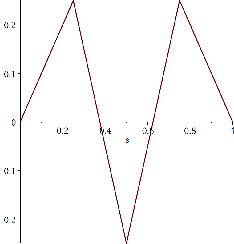
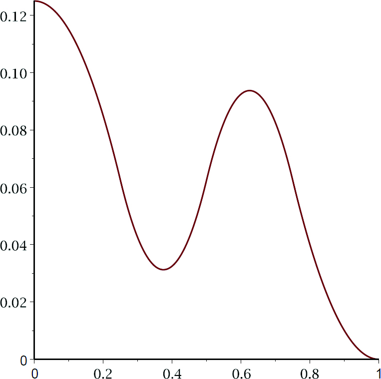
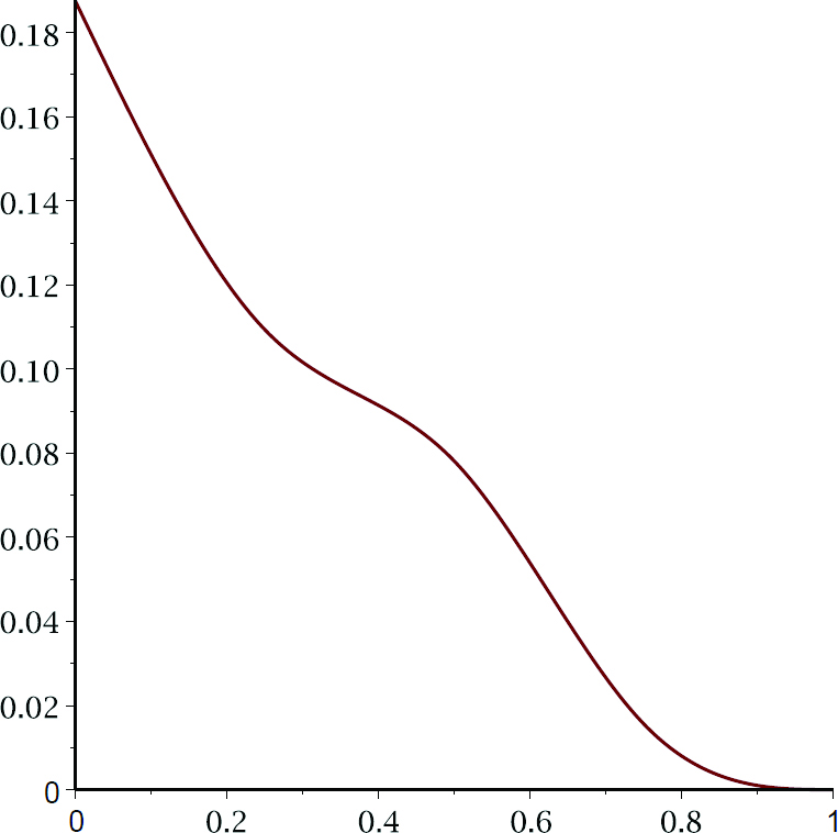
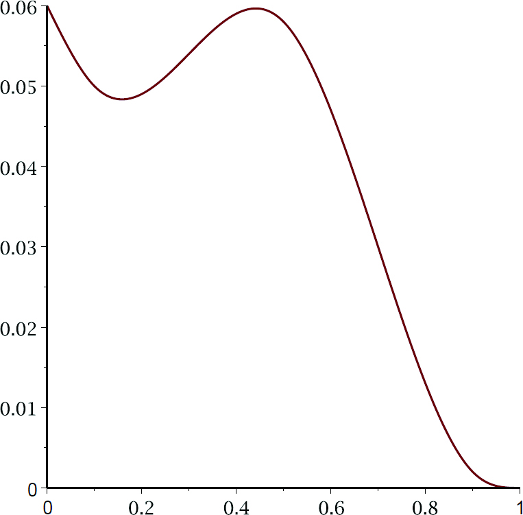
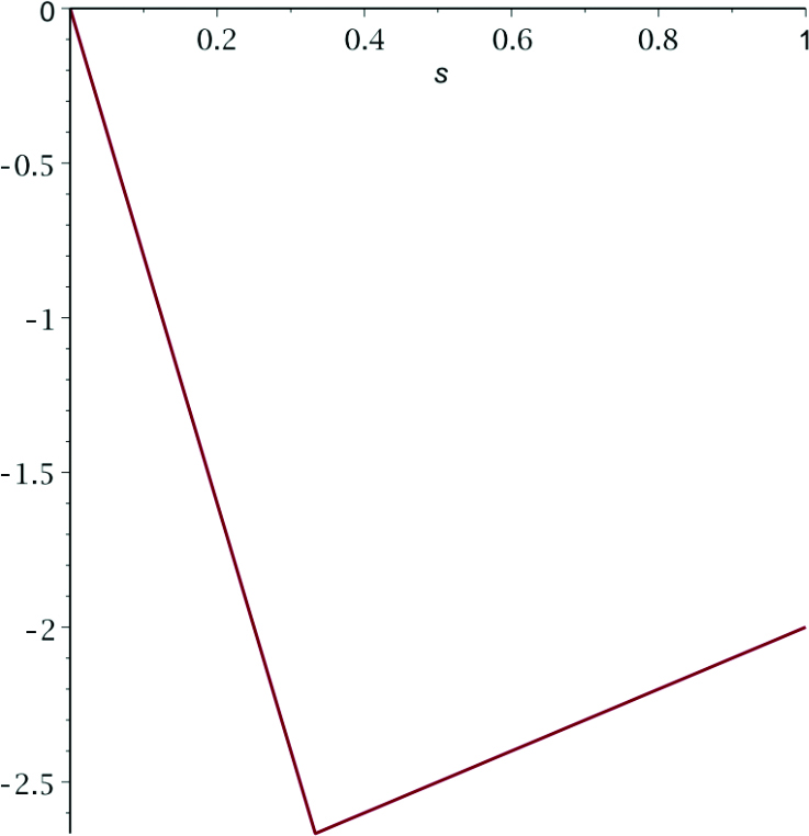
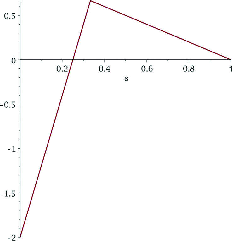
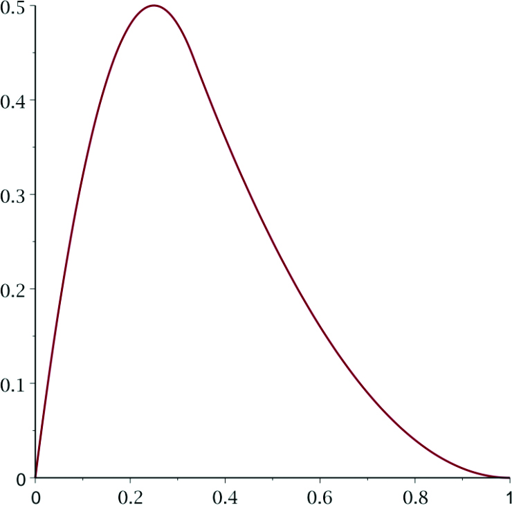
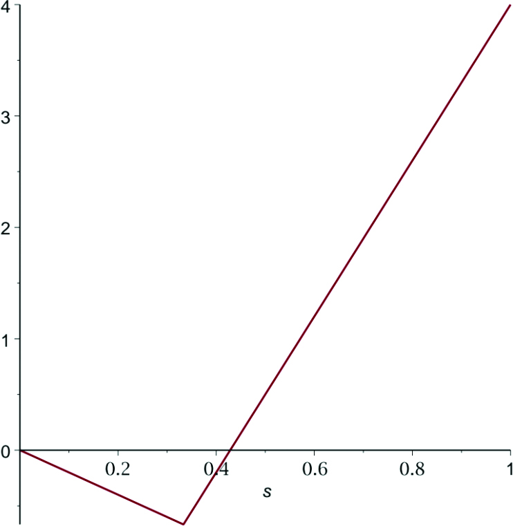
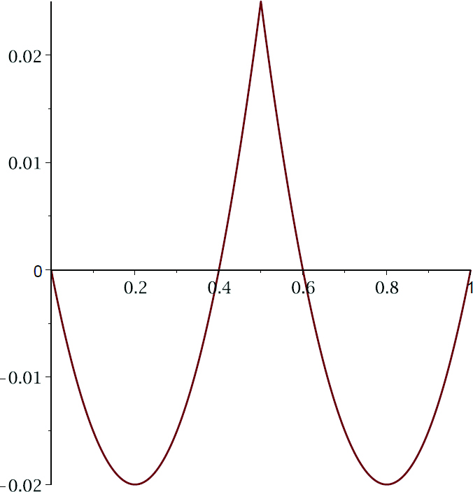
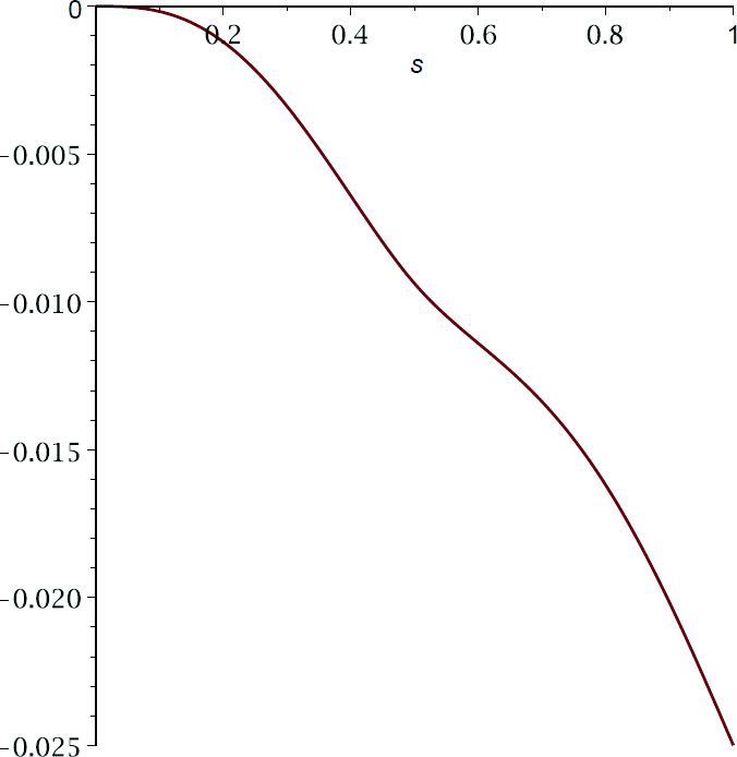
Figure 1
The graphs of the functions
μ
1
+
,
μ
2
+
,
μ
1
−
related to inequality (1.3).
Now, we use Theorem 7 with
λ
=
0
.
The function
μ
1
+
changes its sign in the interval
[
0
,
1
]
(Figure 1 (a)).
This means that not all 2-increasing functions satisfy (1.3).
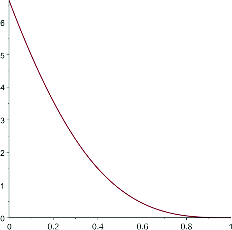
On the other hand, the function
μ
2
+
is nonnegative on
[
0
,
1
]
(Figure 1 (b)).
Therefore, every function belonging to
M
2
+
,
3
+
(
I
)
satisfies inequality (1.3).
Surprisingly, this inequality is also satisfied for
f
∈
M
2
+
,
3
−
(
I
)
.
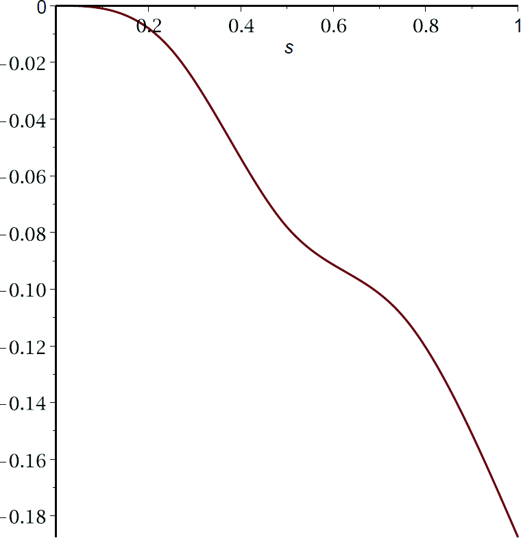
Indeed, using Theorem 7 with
λ
=
1
, it is enough to observe that
μ
0
(
1
)
=
μ
1
(
1
)
=
0
,
μ
2
(
1
)
=
1
8
and
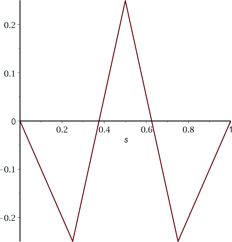
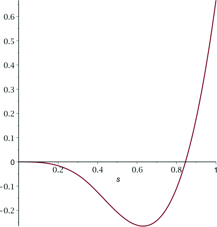
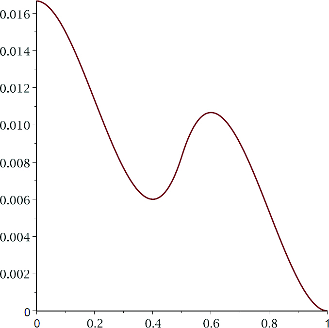
μ
2
−
is nonnegative on
[
0
,
1
]
(Figure 2 (a)).
We also have that
μ
0
(
1
/
2
)
=
μ
1
(
1
/
2
)
=
μ
3
(
1
/
2
)
=
0
and
μ
2
(
1
/
2
)
=
1
/
8
and that
μ
3
−
is nonpositive and
μ
3
+
is nonnegative on
[
0
,
1
]
(Figure 2 (b) and (c)).
Figure 2
The graphs of the functions
μ
2
−
,
μ
3
−
,
μ
3
+
related to inequality (1.3).
Thus, applying Theorem 7 with
λ
=
1
/
2
, it follows that every function belonging to
M
2
+
,
4
+
(
I
)
also satisfies inequality (1.3).
Due to the linearity of inequality (1.3), we finally can obtain that every function 𝑓 belonging to the convex cone
M
2
+
,
3
+
(
I
)
+
M
2
+
,
3
−
(
I
)
+
M
2
+
,
4
+
(
I
)
is a solution to (1.3).
In the next example, we present an inequality where three orders of increasingness must be used to ensure that a given function satisfies this inequality.
Example 4
To deal with the inequality
(5.2)
3
f
(
x
+
9
y
10
)
+
3
f
(
9
x
+
y
10
)
≤
2
f
(
x
)
+
2
f
(
x
+
y
2
)
+
2
f
(
y
)
,
we consider the measure
μ
=
2
δ
0
−
3
δ
1
10
+
2
δ
1
2
−
3
δ
9
10
+
2
δ
1
.
We have
μ
0
(
0
)
=
μ
1
(
0
)
=
0
and
μ
2
(
0
)
=
1
25
.
As in the previous example, every solution of (5.2) must be 2-increasing.
However, this time, both functions
μ
1
+
and
μ
2
+
change their signs in
[
0
,
1
]
(Figure 3 (a) and (b)).
Therefore, we examine
μ
3
+
, and it turns out that it is positive (Figure 3 (c)).
This together with
μ
3
+
(
0
)
=
3
50
>
0
means that (5.2) is satisfied by all functions 𝑓 from
M
2
+
,
3
+
,
4
+
(
I
)
.
Figure 3
The graphs of the functions
μ
1
+
,
μ
2
+
and
μ
3
+
related to inequality (5.2).
Remark 3
In view of Lemma 5, it is clear that if
μ
k
+
is nonnegative for some
k
0
and
λ
∈
[
0
,
1
]
on the interval
[
λ
,
1
]
, then it will be nonnegative for all
k
≥
k
0
on the interval
[
λ
,
1
]
.
This will, however, bring no improvement since all classes of functions obtained in this way will be contained in the previously received.
Thus the procedure is to find the smallest 𝑘 for which
μ
k
+
does not change its sign on the interval
[
λ
,
1
]
.
In the previous two examples, the inequalities were symmetric, resulting in relatively symmetric classes of solutions.
Now, we present an example of a nonsymmetric inequality that will be satisfied by all functions from
M
1
−
,
2
+
(
I
)
and from
M
1
−
,
3
+
(
I
)
.
Example 5
Consider the inequality
(5.3)
9
f
(
2
x
+
y
3
)
≤
8
f
(
x
)
+
f
(
y
)
and the associated measure
μ
=
8
δ
0
−
9
δ
1
3
+
δ
1
.
We have
μ
0
(
0
)
=
0
,
μ
1
(
0
)
=
−
2
which implies that all solutions of (5.3) are decreasing.
The function
μ
0
+
changes its sign, meaning that not all decreasing functions satisfy (5.3).
Further, the function
μ
1
+
changes sign in
[
0
,
1
]
but
μ
1
−
is nonpositive.
(See Figure 4 (a) and (b).) Moreover, we have
μ
0
(
1
)
=
0
,
μ
1
(
1
)
=
−
2
; consequently, applying Theorem 7 with
λ
=
1
, we can see that every function from
M
1
−
,
2
+
(
I
)
satisfies (5.3).
On the other hand, the function
μ
2
+
is nonnegative and
μ
2
(
0
)
=
0
.
Therefore, applying Theorem 7 with
λ
=
0
, we obtain that every function from
M
1
−
,
3
+
(
I
)
also satisfies (5.3).
In conclusion, by the linearity of the functional inequality, it follows that every function from the convex cone
M
1
−
,
2
+
(
I
)
+
M
1
−
,
3
+
(
I
)
fulfills (5.3).
Figure 4
The graphs of
μ
1
+
,
μ
2
+
,
μ
1
−
related to inequality (5.3).
Observe that, until now, the only class of solutions obtained with the use of 𝜆 different from numbers 0 or 1 was
M
2
+
,
4
+
from Example 3, where
λ
=
1
2
was used.
However, even in that example, the functions
μ
3
+
,
μ
3
−
were positive, resp. negative on the whole interval
[
0
,
1
]
.
Observe that the assumption of Theorem 7 is weaker.
In the next example, we will use that theorem in its full strength.
Example 6
Consider the inequality
(5.4)
9
f
(
2
x
+
y
3
)
≤
2
f
(
x
)
+
7
f
(
y
)
and the measure
μ
=
2
δ
0
−
9
δ
1
3
+
7
δ
1
.
Here we have
μ
0
(
0
)
=
0
and
μ
1
(
0
)
=
4
.
This means that every solution of (5.4) is increasing.
The positivity of
μ
1
−
implies that every function from
M
1
+
,
2
−
satisfies (5.4).
Figure 5
The graphs of the functions
μ
1
+
,
μ
2
+
and
μ
2
−
connected with inequality (5.4).
The function
μ
2
−
, on the other hand, changes its sign on
[
0
,
1
]
, and therefore, we cannot use here Theorem 7 with
λ
=
1
.
We will use here
λ
=
3
4
.
We have
μ
0
(
3
4
)
=
0
,
μ
1
(
3
4
)
=
4
,
μ
2
(
3
4
)
=
0
.
Further, we have
μ
2
−
(
τ
)
≤
0
for
τ
∈
[
0
,
3
/
4
)
and
μ
2
+
(
τ
)
≥
0
for
τ
∈
(
3
/
4
,
1
]
;
see Figure 5 (b) and (c).
Therefore, using Theorem 7, we get that (5.4) is also satisfied by all
f
∈
M
1
+
,
3
+
.
In conclusion, by the linearity of the functional inequality, it follows that every function from the convex cone
M
1
+
,
2
+
(
I
)
+
M
1
+
,
3
+
(
I
)
fulfills (5.4).
Remark 4
As we can see, if we are given a functional inequality of the form
(5.5)
a
1
f
(
α
1
x
+
(
1
−
α
1
)
y
)
+
⋯
+
a
n
f
(
α
n
x
+
(
1
−
α
n
)
y
)
≥
0
,
then using Theorem 7, we can find a class of functions that satisfy this inequality.
Interestingly, if the classical condition needed for an 𝑛-increasing ordering is satisfied, we get only one class of solutions.
Still, if this is not the case, then different classes of functions may satisfy that inequality.
Given the above remark, we may say that the results obtained in this paper yield a step toward a complete solution of inequality (5.5).
However, the applications of our results are not limited to dealing with inequalities of that kind.
For example, it is well known that the Bullen inequality
1
y
−
x
∫
x
y
f
(
t
)
d
t
≤
1
4
f
(
x
)
+
1
2
f
(
x
+
y
2
)
+
1
4
f
(
y
)
holds for all 2-increasing (i.e., convex) functions 𝑓 and that
1
y
−
x
∫
x
y
f
(
t
)
d
t
≤
1
6
f
(
x
)
+
2
3
f
(
x
+
y
2
)
+
1
6
f
(
y
)
is satisfied by all 4-increasing functions (cf. [1]).
The right-hand side of the above inequalities is of the form
a
f
(
x
)
+
(
1
−
2
a
)
f
(
x
+
y
2
)
+
a
f
(
y
)
,
with
a
=
1
4
,
1
6
.
It is natural to ask what happens for other values of 𝑎.
We will consider such a situation in the following example.
Example 7
The inequality
(5.6)
1
y
−
x
∫
x
y
f
(
t
)
d
t
≤
1
5
f
(
x
)
+
3
5
f
(
x
+
y
2
)
+
1
5
f
(
y
)
is satisfied by all
(5.7)
f
∈
M
2
+
,
3
+
(
I
)
+
M
2
+
,
3
−
(
I
)
+
M
2
+
,
4
+
(
I
)
for all
x
,
y
∈
I
with
x
<
y
.
Indeed, consider the measure
μ
=
1
5
δ
0
+
3
5
δ
1
2
+
1
5
δ
1
−
ℓ
,
where ℓ is the Lebesgue measure restricted to the measurable subsets of
[
0
,
1
]
.
Then we have
μ
0
(
0
)
=
μ
1
(
0
)
=
0
and
μ
2
(
0
)
=
1
60
.
Figure 6
The graphs of the functions
μ
1
+
,
μ
1
−
,
μ
2
+
,
μ
2
−
,
μ
3
+
,
μ
3
−
connected with inequality (5.6).
Further, the functions
μ
1
+
and
μ
1
−
change sign in
[
0
,
1
]
(Figure 6 (a) and (b)); therefore, the inequality is not satisfied by all 2-increasing functions.
On the other hand,
μ
2
+
and
μ
2
−
are nonnegative on
[
0
,
1
]
(Figure 6 (c) and (d)).
Therefore, applying Theorem 7 with
n
=
3
and
λ
∈
{
0
,
1
}
, we obtain that (5.6) is satisfied by all
f
∈
M
2
+
,
3
+
(
I
)
and
f
∈
M
2
+
,
3
−
(
I
)
, respectively.
The function
μ
3
vanishes at
λ
=
1
/
2
and condition (b) (i) of Theorem 7 with
n
=
4
and
λ
=
1
/
2
is satisfied (Figure 6 (e) and (f)); therefore, (5.6) also holds for all
f
∈
M
2
+
,
4
+
(
I
)
.
Using the linearity of (5.6), it now follows that it holds for all 𝑓 satisfying (5.7).
 and
Tomasz Szostok
and
Tomasz Szostok