Transient Analysis of Falling Cylinder in Non-Newtonian Fluids: Further Opportunity to Employ the Benefits of SPH Method in Fluid – Structure Problems

MohammadMahdi Kamyabi; S.A. Ramazani Ahmad; Ata Kamyabi

doi:10.1515/cppm-2016-0044

Article Publicly Available

Transient Analysis of Falling Cylinder in Non-Newtonian Fluids: Further Opportunity to Employ the Benefits of SPH Method in Fluid – Structure Problems

MohammadMahdi Kamyabi , S.A. Ramazani Ahmad and Ata Kamyabi

Published/Copyright: January 10, 2017

Published by

Become an author with De Gruyter Brill

Submit Manuscript Author Information

From the journal Chemical Product and Process Modeling Volume 12 Issue 1

Abstract:

Smoothed particle hydrodynamics (SPH) was applied to simulate the free falling of cylindrical bodies in three types of fluids including Newtonian, generalized-Newtonian and viscoelastic fluids. Renormalized derivation schemes were used because of their consistency in combination with the latest version of no slip boundary condition to improve the handling of moving fluid-structure interactions (FSIs). Verification of the method was performed through comparing the results of some benchmark examples for both single and two phase flows with the literature. The effects of some parameters such as the viscosity of the Newtonian fluid, the n index of the power-law fluid and the relaxation time of the Oldroyd-B fluid along with the diameter of the cylinder on the falling history were investigated. Achieving reasonable results, SPH method was proven to be suitable for simulating moving fluid-structure boundaries independent of the fluid type.

Keywords: SPH method; fluid-structure interaction; Non-Newtonian fluids; Boundary treatment

1 Introduction

Understanding the rheology of non-Newtonian fluids is important not only for their wide applications but also for powerful theoretical background needed to be covered. In addition to the non-linear nature of such fluids, intricate geometries which usually appear in their processing steps or characterization experiments, increase complexity. Although it seems easy in the first sight, falling body through the fluid is one popular case of these complex geometries. Complexity comes from the difficulties attributed to the existing fluid-structure interactions (FSIs). For example, classic computational fluid dynamics (CFD) methods have difficulties in simulation of translational motion of the fluid-structure interfaces, because capturing the interface is not easily possible using these methods [1].

In a case of non-reactive falling body, the only important issue is hydrodynamics. Accurate calculation of hydrodynamic forces swapped between the solid body and fluid is required in order to predict the falling behaviour. These forces have been conceptually determined for many years. Governing equations, especially momentum conservation law, describe the relationship between these forces and the flow parameters. In the steady conditions and as a simple way, the flow of the fluid on the stationary solid object can be considered instead of the flow of the falling object through the static fluid. Using the same simplification, well-known Stokes equation for terminal velocity of falling spheres has been obtained as: VStokes=2gR2ρs−ρf9μ (corresponding to drag force: FDStokes=6πμRVStokes) [2]. Where g is the gravity acceleration, ρ_s and R are the density and radius of the sphere respectively, ρ_f and µ are the density and viscosity of the fluid Respectively. This equation which is frequently used in falling ball viscometers for determining the viscosity of the Newtonian fluids, may be considered as the outcome of the first attempts on the modeling of falling problems.

Researchers have tried to reconsider simplifying assumptions which are necessary for the validity of the Stokes equation. These assumptions are Newtonian fluid, steady-state condition, low Reynolds numbers, spherical solid shape and most important of them: not considering the translational moving of the solid (see [3, 5]). After eliminating simplifying assumptions, the system of the governing equations will be generally described with a set of time dependant partial differential equations (PDEs). Non-linear nature of such PDE system, usually requires the application of numerical approaches for its solution.

In this regard, Feng et al. [6] used finite element method (FEM) to simulate falling of a 2-D cylinder in Newtonian fluid at moderate Reynolds numbers. As with non-spherical bodies, falling of elliptical particles in Newtonian fluid has been investigated by Xia et al. [7] and simulations of falling a wedge and also cubic solids have been carried out by Liu et al. [8] for Newtonian fluid, via incompressible SPH (ISPH) method. Reconsidering Newtonian fluid assumption, falling behaviour of a solid sphere in the Oldroyd-B fluid has been studied by using FEM [9, 10]. A good review on experimental and numerical investigations of transient and steady motion of falling spheres in viscoelastic fluids have been published by McKinley et al. [11]. This work is actually the complementary to the previous review [12].

Assuming stationary body instead of falling one becomes meaningless when transient solution is of interest. Therefore, applying an accurate and fast computational approach becomes essential due to measure instantaneous mutual effects between fluid and solid. Considering these mutual effects, this approach should be able to capture moving of the interface correctly over the time [13]. Although falling problem has been investigated extensively, it has often been treated with conventional mesh based Eulerian methods. It is helpful to note that, there are two fundamental frames for describing governing equations: Eulerian and Lagrangian frames [14]. Through the Eulerian framework, coordinates are fixed in the space while coordinates move with the system in the Lagrangian viewpoint. In the Lagrangian formulations, the complexity of the numerical methods is reduced due to vanishing convective terms. Furthermore, in two phase problem of moving fluid-structure interfaces, the interface does not cut the computational mesh which facilitates treatment of such FSIs [13]. Despite such benefits, most Lagrangian methods have difficulties while tracking fluid segments, such as non-physical penetration of the fluid through the solid walls and oscillating results in the pressure field [15].

Meshless methods are particularly useful types of Lagrangian computational methods which have been applied to simulate falling problems [8, 13, 16, 17, 18, 19, 20, 21]. Meshless methods do not face failures such as mesh cutting off and interface dispersion. These benefits are supposed to be appropriate for simulating transient falling problem as a moving boundary FSI case. This is the main idea of the present work. Particle-based meshless methods engage a set of discrete particles to represent the state of the system and to record its deformation [14]. Smoothed particle hydrodynamics (SPH), as one of the oldest and most popular particle-based meshless methods was first applied to simulate astrophysical flows [22, 23]. Utilizing this method successfully in many engineering problems [24, 25] lead to constant improvements in the accuracy and stability of SPH.

The current work deals with solving the 2-D unsteady falling cylinder flow problem in Newtonian, generalized-Newtonian and viscoelastic fluids by using a modified version of weakly compressible SPH (sometimes called WCSPH). These modifications include using the most consistent discretization schemes for spatial derivatives in the flow equations and using the recent implemented version of solid boundary condition introduced by Fatehi et al. [15]. The code was written in C++ and the results were transferred to paraView software for post-processing. Validation of the method is carried out through comparison of the results with reliable reports in the literature. After obtaining rational results from a parametric study, it is proven now, using SPH in its most progressive version, falling problem as a kind of physical FSI problem can be simulated correctly and more easily than usual mesh based methods. It is also concluded that, the applicability of the method is not limited by the fluid type.

2 Governing equations

Since the falling problem is a two phase problem, governing equations for both fluid and solid phases were considered. The cavity example which was examined for the purpose of validation is a one phase problem. Therefore, conservation equations of the fluid were enough to be considered. It would be beneficial to mention that the system of equations was solved numerically at each time step since transient solution was intended.

2.1 Fluid description

SPH method requires the mass and momentum conservation equations to be written in a Lagrangian form. Thus the following equations were solved:

– Conservation of mass:

(1)dρdt=−ρ∇.V

In which ρ is the density of the fluid and V is the velocity vector.

– Conservation of linear momentum:

(2)ρDVDt=∇.T+ρg+f

Where g is gravity acceleration, f is the net of all other body forces (which was zero in the present study) and T is the total stress tensor which can be written as:

(3)T=−PI+τ

In this equation, P is the mechanical pressure, I is the identity matrix and τ is the shear stress tensor. As mentioned before, eq. (2) is written in Lagrangian form in which the DDt operator is the material or total time derivative and it is defined as the eq. (4):

(4)DDt=∂∂t+V.∇

2.1.1 Incompressibility

The ratio of the flow velocity to the local sound speed is known as Mach number. Flows with Mach number less than 0.1 are supposed incompressible which means density of the fluid does not change considerably along the flow or with the time [19].

Commonly two general ways exist for applying incompressibility of the flow. The more common way is to suppose the fluid flow completely incompressible and rewrite eqs (1) and (2) with considering this assumption. Thereupon density is removed from the equations and system of the equations becomes close. Another way which was also used in this work is to suppose an incompressible flow like a compressible one but with very small compressibility. Weakly compressible SPH or briefly WCSPH is a version of SPH which uses this approach. Applying this way, it is needed to define another equation due to system of equations becomes close. This equation is the equation of state (EOS) which expresses pressure relationship with density. One of the most used EOS equations for the fluids is:

(5)P−P0=C2ρ−ρ0

Where P₀ is the pressure of the fluid when its density is ρ₀and C is the artificial sound speed in the fluid. Sound speed is artificial because it should be chosen by the user in a way that the incompressibility condition (Mach number less than 0.1) is satisfied.

2.1.2 Constitutive equations

The Newtonian model which is the simplest form of the mathematical models for the viscous fluids describes the shear stress tensor as eq. (6).

(6)τ=μD

Where D is the rate of the deformation tensor and is defined as:

(7)D=∇V+∇VT

Generalized-Newtonian fluids are another type where their shear rate is a nonlinear function of the rate of deformation tensor. However shear rate is still independent of history of deformation. There are several models for describing these fluids. Power-law equation which was chosen to represent Generalized-Newtonian fluid in this work, describes τ as follow:

(8)τ=η0Dn−1D

Where η₀ is the consistency index and |D|is the size of the rate of the deformation tensor which is defined as follow:

(9)D=(12D:D)

Viscoelastic fluids exhibit both elastic and viscous behaviours. As a result, shear rate of these fluids is dependent on the history of deformation. In the present work, Oldroyd-B constitutive equation is used in order to represent a viscoelastic fluid. Its formulation is [26]:

(10)τ+λ1τ∇=ηD+λ2D∇

Where λ1 is the relaxation time, λ2 is the retardation time, η is the zero shear rate viscosity and τ∇ is the upper convected derivative of τ. The upper convected derivative of any symmetric tensor like A is defined as follow in a Lagrangian coordination system:

(11)A∇=∂A∂t−A.∇V−∇VT.A

When λ2=0, eq. (10) reduces to upper convected Maxwell (UCM) model, and if λ1=λ2=0, it represents the Newtonian fluid with the viscosity η. If the stress tensor τ decomposed into a viscoelastic component τ_p and a purely viscous component τ_s then [27]:

(12)τ=τp+τs

where

(13)τp+λ1τ∇p=ηpD

and

(14)τs=ηsD

Here, η_p is the viscosity of the viscoelastic contribution, and η_s is the viscosity of

Newtonian contribution such that the following equations show the relationship between the parameters.

(15)η=ηp+ηs

and

(16)λ2=ηsηλ1

Then, by substituting eqs (13) and (14) into eq. (12) and using eqs (15) and (16) results in eq. (10), the momentum conservation equation can be written as eq. (17).

(17)ρDVDt=−∇P+∇.τp+ηs∇2V

2.2 Solid description

The common second law of the Newton governs on the solid body motion. Hence the following equation determines the solid body behaviour:

(18)Fs=msdVsdt

Where F_s, m_s and V_s are the total force exerted on the solid cylinder, total mass and velocity of the solid cylinder respectively. As it is clear, knowing all the exerted forces on the solid body is necessary in order to calculate its instantaneous velocity.

2.3 Fluid-solid coupling

As it was mentioned before, the accurate results would be achieved if only an efficient algorithm ensures the correct implementation of continuous interactions between solid and fluid. Because the rigid solid was considered, it can’t be deformed. Therefore the solid could be defined only with the fluid boundary particles which were stuck to the solid surface (see Figure 1). The fluid-solid coupling was carried out through these wall particles as well. When the total amount of the forces exerted on the solid and subsequently the velocity of the solid is computed, the wall boundary particles give the same velocity as the velocity of the solid and move across the fluid. Now the fluid equations are solved under the influence of these particles movement. Again the total forces exerted on the solid are computed under the new conditions and this algorithm is going on. Therefore, a two-way coupling was applied by this algorithm.

Figure 1:

Arrangement of SPH particles on the fluid-solid interface.

Determining these forces numerically and implementing SPH for solving the governing equations are discussed in the Section 3.

2.4 Dimensionless numbers

Distinguishing viscous and elastic effects, it is needed to employ dimensionless numbers involving these characteristics. In this regard, Reynolds (Re) and Deborah (De) numbers are defined as below:

(19)Re=ρVdη

(20)De=λ1VR

Where |V|is the size of the velocity vector of the cylinder, d is the diameter of the cylinder, R = d/2 is its radius and other parameters have been introduced before. In this problem, Deborah number is actually the ratio of the fluid relaxation time to the residence time of any element of the fluid near the cylinder [11].

3 Numerical implementation

Using SPH, particles are computational points and carry fluid quantities such as mass, velocity and pressure. SPH method is built on the concept of interpolation where interpolated value <u> at position r is computed as:

(21)<uhr>=∑jωjurjWrj−r,h

Where u is each arbitrary field function and ω_j is the volume of the neighbouring particle j. Particle j is the neighbour if it is within the circular area around a point at r with radius h. W is a positive smoothing or kernel function representing Dirac delta function [23]. In all simulations of this work, Quintic Wendland kernel function was used which is described as below [28]:

(22)W(r,h)= W0×{(1−rh)4(4rh+1)00<rh≤1rh>1

Where r = |r_j -r|and W₀ is 7/πh² for two dimensional problems.

3.1 SPH discretization

Nowadays it is vivid that most derivative schemes used in SPH are not consistent. This means the truncation error of them would not reach zero when space between particles goes to zero. A consistent first-order scheme which is introduced by Randles and Libersky [24] was used for computing first spatial derivatives ∇P and ∇V. According to this scheme, the numerical approximation of the first derivative of any arbitrary parameter like u can be obtained as eq. (23):

(23)∇ui=∑jωjuj−uiBi.∇Wij

Where Wij=Wrij,h is the value of smoothing or kernel function of particle i at the position of particle j. Moreover, B_i which is defined in eq. (24) is a renormalization tensor.

(24)Bi=−∑jωjrij∇Wij−1

rij=ri−rj is the distance vector between particles i and j.

It is shown that this scheme is consistent and converges linearly as δ goes to 0 for a constant ratio δ/h, where δ denotes the SPH particles spacing [13].

For computing ∇2V, the second derivative approximation is required. The following equation which is confirmed by Basa et al. [29] for its accuracy, was used for second derivatives:

(25)∇.∇ui=∑j2ωjui−ujrijeij.∇Wij

where

(26)eij=rijrij

is the unique position vector between two particles.

As mentioned before, computing the total force exerted on the solid body is necessary. F_s in eq. (18) is the summation of pressure, viscous and gravity forces where in the discrete form is calculated from eq. (27).

(27)Fs=∑j−Pjnj+nj.τjdsj+ms−ρVs‾g

This summation is on the all particles sticking to the surface of the solid body which are visible in the Figure 1. Vs‾ is the volume of the solid, njis the outward unit normal vector to the solid surface at position of particle j and dS_j represents the area which is the portion of particle j on the solid surface. This area is actually the total surface of the solid divided by the total number of particles which are forming the surface.

Separately writing gravity and buoyancy in the above equation is the recommendation of Hashemi et al. [13] since it is appropriate for more computational efficiency.

3.2 Interface boundary treatment

Appropriate implementation of boundary conditions plays an important role in the accuracy of the method. Although no-slip condition was used for all fluid-structure boundaries, there are several different techniques to apply this condition in the SPH method. Using opposing force [30], adding several layer dummy (ghost) [31], or mirror [32] particles and solving momentum equation on the one layer of particles [15] are some kinds of these techniques. The last one suggests calculating the pressure of wall boundary particles from momentum equation. This leads the acceleration of each boundary particle in the normal direction to the wall becomes zero and penetration through walls will not occur. The same technique was used in present work. Using this way, there is no need for several boundary layers of particles and the solid-fluid interface was represented only by one layer of SPH particles as is shown in Figure 1.

According to this technique, the fluid equation of motion should be solved in order to find the pressure and density of a boundary particle. Adjacent to solid surfaces, the momentum conservation equation can be rewritten as:

(28)∇Pρ.n=−dVdt.n+∇.τρ.n+g.n

Where n is the outward unit normal vector to the solid surface. For the boundary particle i, n_i is equal to the normal summation of the kernel gradients as eq. (29) shows [24].

(29)ni=∑jωj∇Wij∑jωj∇Wij

Discretizing the pressure gradient term in eq. (28) for particle i, and rearranging the equation, pressure of particle i at (m + 1)^st time step is obtained explicitly from this equation:

(30)Pim+1=(∑jPjm+1ρijB.∇Wij).ni+dVidt.ni−∇.τρim+1.ni−g.ni∑j1ρijB.∇Wij.ni

The term dVidt is the acceleration of the boundary particle i. According to the no slip boundary condition, the acceleration is equal to the corresponding solid body acceleration. Therefore the values of dVidt obtains from eq. (18) at each time step for each boundary particle i.

3.3 Time integration

Governing equations are written in transient format. It means they must be solved with time propagation. Considering momentum conservation equation, velocity of each fluid particle is calculated directly from the following equation for the Newtonian fluid:

(31)Vim+1=Vim+Δt−∇Pρm+ν∇.∇Vm+gi

The equation (32) is showing the velocity relation of each particle for the power-law fluid:

(32)Vim+1=Vim+Δt−∇Pρm+η0ρ∇V+∇VTn−1.∇Vm+gi

For the Oldroyd-B fluid, stress tensor is calculated according to this equation:

(33)τpm+1+λ1τpm+1−τpmΔt−τpm.∇Vm−∇VTm.τpm=ηp∇Vm−∇VTm

After ∇.τis calculated, it is substituted in momentum eq. (2) to update fluid velocity. Velocity of solid surface particles comes from this equation:

(34)Vim+1=Vim+Δt.dVsdt

Where dVsdt denotes the acceleration of solid body and obtains from solving eq. (18).

As it is clear, time integration of velocity is performed through explicit formulation. Although there are more accurate schemes for time propagation, explicit first order simple scheme is sufficient. More complex schemes will not necessarily lead to accuracy in results because spatial derivative schemes are first order and they are the controller of the precision. Therefore no serious gain would achieved while more computational cost was imposed if that schemes were employed. At the end of each time step, density of each particle gets implicitly updated by eq. (35) in order to be used in the next time step.

(35)ρim+1=ρim+Δt−ρ∇Vm+1i

After that, particles move according to their new velocities through the time and get new arrangements according to eq. (36). Since Reynolds number in the present simulations was low, the deformations were relatively low and particles were not accumulated or dispersed very harshly. Therefore rearrangement techniques were not needed.

(36)rim+1=rim+ΔtVim+1

It is necessary to mention that, the time step was chosen based on the criteria suggested by Shao and Lo [24].

4 Validation study

Validation of the present method was carried out through comparison of its results with two specific cases in the literature. These cases were selected in order to cover both single and two phase problems.

4.1 Single phase flow in a cavity

The first problem is driven flow in a cavity in which fluid confined in a square enclosure gets affected by the moving of upper surface according to Figure 2. Different fluid patterns are expected based on Reynolds number. The problem assumptions that are used in the present work are as below:

Fluid is Newtonian

Reynolds number is 100

No slip boundary condition is applied to the walls; it means that:

u=U,v=0attopwall

(37){u=U,v=0attopwallu=v=0atotherwalls

Figure 2:

Schematic of the cavity problem.

Comparison of the results of the present method with the Ghia et al. [33] is shown in the Figure 3. These results include normalized horizontal velocity (u) and vertical velocity (v) along the related normalized centrelines. Normalization was done for the velocity and position with the top velocity (U) and the length of the square respectively. As it is clear, good agreement between the results is observed. This helped to ensure that, the method is applicable in general and the code is correct, at least for one phase fluid flows.

Figure 3:

Comparison of the results for cavity problem with Ghia et al. [33]: Normalized vertical velocity along the horizontal centerline of cavity (up) and Normalized horizontal velocity along the vertical centerline of cavity (down).

4.2 Falling cylinder in Newtonian fluid

The problem of the falling cylinder in a Newtonian fluid has been chosen in order to ensure that the boundary and derivative formulas are applied correctly and the two-phase code works accurately. Figure 4 shows the comparison of the velocity of the cylinder with the results reported by Hashemi et al. (SPH method) [13] and Glowinski et al. (Direct Numerical Simulation coupled with Finite Element Method (DNS-FEM)) [34]. All conditions of the problem are the same. According to the Figure 5 these conditions are:

Domain dimensions are H = 0.06 m and L = 0.02 m

Diameter of the Cylinder is d = 0.0025 m

Density of the solid cylinder is ρ_s = 1,250 kg/m³

Density of the fluid is ρ_f = 1,000 kg/m³

Viscosity of the fluid is µ = 0.01 Pa.s

Figure 4:

Comparison of the velocity of the falling cylinder in Newtonian fluid with Glowinski et al. (DNS-FEM) [34] and Hashemi et al. (SPH method) [13] results.

Figure 5:

Schematic of the falling cylinder problem.

Good agreement observed, make it easy to ensure of our method for correct simulation of two phase flows specially moving FSIs.

5 Results and discussion

5.1 Inter-particle spacing

Average nearest-neighbour spacing of SPH particles is an important parameter because either very short or long spacing lead to wrong answers. This issue is also confirmed by many researches (for instance see [29]). In the present work, simulations have been carried out with different initial distances, and finally the appropriate distance δ_bst has been selected. This spacing is chosen based on considering convergence criteria and after obtaining the best agreement of the results with the results in the literature which were explained in the previous section. δ_bst obtained equal to 0.357h, where h is the smoothing length.

In the following, some of the most important parameters which affect the falling behaviour are investigated and the results are reported. These parameters include fluid viscosity (in the Newtonian case), fluid shear-thinning and shear-thickening nature (in the power-law case), fluid relaxation time and cylinder’s diameter (both in the Oldroyd-B case). All the geometrical parameters are the same as the parameters mentioned at the Section 4.2 unless directly addressed.

5.2 Effect of the viscosity

Viscosity of the fluid directly affects the transient and steady velocities of the cylinder due to changing of the viscous forces exerted on the cylinder. Changing viscosity, simulations of Newtonian case were carried out and the results of the velocity of the cylinder versus time is shown in Figure 6. The effect of the viscosity is hidden in the reported Reynolds numbers so that higher Reynolds number is the outcome of less viscosity and vice versa. The Reynolds numbers are calculated based on terminal velocities.

Figure 6:

Velocity of the falling cylinder at different Reynolds numbers (influence of viscosity).

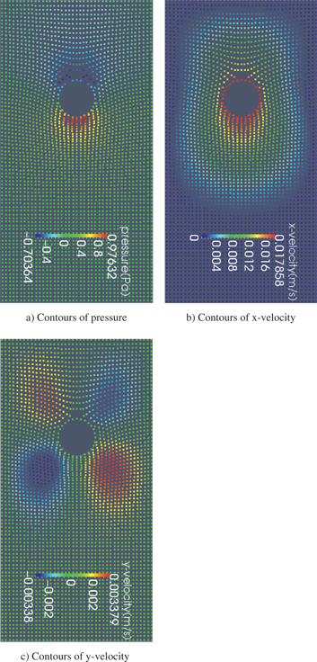
According to this figure, both transient and steady velocities of the cylinder decrease with increasing the viscosity of the fluid. This is because of enhancement in viscous resistant forces. Contours of velocity and pressure in a specific time are also shown in Figure 7 for better perception of the hydrodynamic patterns. According to this figure, pressure is magnified in front of the cylinder and it is reduced at the back as it was sensible and expected. Velocity contours are showing the flow path obviously.

Figure 7:

Contours of pressure and velocity components in Newtonian fluid (a) Contours of pressure (b) Contours of x-velocity (c) Contours of y-velocity.

5.3 Effect of shear-thinning and shear-thickening

The n index in power-law equation (eq. (8)) indicates shear-thinning (for n < 1) and shear-thickening (for n > 1) nature of the fluid. If n = 0 it represents Newtonian fluid. The effect of this parameter on the settling velocity of the cylinder was also investigated and is compared in Figure 8 where all other operating conditions are the same. According to the results, velocity of the falling cylinder in shear-thinning fluid at each time is significantly more than its amount in Newtonian fluid and falling velocity in Newtonian fluid is more than shear-thickening one. These observations are rational because apparent viscosity decreases by increasing deformation in shear-thinning fluids while this behaviour is seen reversely in shear-thickening fluids. Hence lower and higher viscous resistant forces against falling are generally expected for shear-thinning and shear-thickening fluids respectively.

Figure 8:

Effect of shear-thinning and shear-thickening nature of the fluid on the velocity of the falling cylinder (influence of n index).

5.4 Effect of the relaxation time

Relaxation time, as the characteristic parameter of viscoelastic fluids, generally indicates the scale time which the fluid needs to relax under any certain change. According to the eq. (10), it is expected that, this parameter affects the stresses in the fluid which finally leads to change in the flow patterns and velocity magnitude of the cylinder.

In the Figure 9, velocity of the falling cylinder is plotted as a function of time at various Deborah numbers. For each case, Deborah number is calculated based on the terminal velocity. The effects of relaxation time are latent in Deborah as eq. (20) suggests. Exploring the chart for each case, there are undershoots in the velocity amounts before the cylinder reaches its steady terminal velocity. In the Figure 10, normalized velocity versus dimensionless time is compared with the other available results in the literature ([9, 10, 35]). As it is obvious, this undershoot in transient velocity profile (overshoot in dimensionless velocity) is valid, but its amount varies. A meaningful quantitative comparison cannot be made because of matching of all various effective parameters is impossible, as Feng et al. [10] also mentioned. It is helpful to note that, normalized velocity and dimensionless time, was obtained from eqs (38) and (39) respectively.

(38)V=VxVx,final

(39)t=tλ1

Figure 9:

Velocity of the falling cylinder at different Deborah numbers (influence of relaxation time).

$Figure 10: Comparison of the normalized falling velocity in three studies. Present work: Re = 0.42, De = 0.374, Fr = 41.89, ρs/ρf = 1.25. Feng et al. [10].: Re = 0.0451, De = 0.2255, Fr = 10.36, ρs/ρf = 26.74. Bodart and Crochet [9]: Re = 1.2936, De = 1.986, Fr = 4.967, ρs/ρf = 7.162. Becker et al. [35]: Re=5.4×10−2,${\bf{Re}} = 5.4 \times {10^{- 2}},$ De = 0.402, Fr is not given (Fr is Froude number and defined asgd/Vx,final2${\bf{gd}}/{\bf{V}}_{{\bf{x}},{\bf{final}}}^2$).$

Figure 10:

Comparison of the normalized falling velocity in three studies. Present work: Re = 0.42, De = 0.374, Fr = 41.89, ρ_s/ρ_f = 1.25. Feng et al. [10].: Re = 0.0451, De = 0.2255, Fr = 10.36, ρ_s/ρ_f = 26.74. Bodart and Crochet [9]: Re = 1.2936, De = 1.986, Fr = 4.967, ρ_s/ρ_f = 7.162. Becker et al. [35]: Re=5.4×10−2, De = 0.402, Fr is not given (Fr is Froude number and defined asgd/Vx,final2).

In addition to the numerical results, many experimental evidences also confirmed the overshoot existence (for a comprehensive review see [12]).

Complex relationship is observed between velocity and Deborah number. Although Reynolds number is another effective parameter, it was tried to fade its effect by considering the simulations at approximately the same Reynolds numbers. Increase in velocity by increasing the Deborah number is seen for all cases only at the early times after releasing the cylinder but there are some differences for later times: Generally increase in velocity by increasing the Deborah number is also observed for Deborah numbers less than 1.44 but this trend is reversed at higher Deborah numbers. Contours of velocity and pressure for a viscoelastic case are shown in the Figure 11.

Figure 11:

Contours of pressure and velocity components for viscoelastic fluid (a) Contours of pressure (b) Contours of x-velocity (c) Contours of y-velocity.

5.5 Effect of the diameter

Simulations of viscoelastic cases were applied for two different sizes of cylinder diameters: 0.0025 m and 0.00125 m. Influence of this parameter on the velocity of the cylinder has been reported in Figure 12 where the velocity of the cylinder is shown versus time.

Figure 12:

Velocity of the falling cylinder at two different diameters of cylinder.

According to this figure, the larger cylinder experienced more falling velocity which means more net force is exerted on the larger one. Although the larger cylinder faces with more resistant surface forces, its more weight causes further driving force and therefore the motion has been impressed more by the weight.

6 Conclusion

In the present work, a progressive version of weakly compressible SPH method was used to demonstrate its ability for accurate simulating of moving FSI problems. First, the accuracy of this method was examined successfully for the cavity case as a benchmark problem, to prove its ability for simulating one phase fluid flows. The method showed its reliability also for two phase flows (especially moving FSI problems) through good agreement of its results for falling cylinder in the Newtonian fluid with available results in the literature. The method was then applied to simulate falling cylinder in the Newtonian, power-law and Oldroyd-B fluids at various conditions. Improved outcomes were obtained such that no non-physical oscillating values in pressure field were seen and penetration inside the solid cylinder did not occur. This improvement is significant in the field of particle-based meshless methods.

In addition to proving the potential of this method for simulating such FSI problems, other most important practical conclusions are classified as the following items:

Fluid characteristics such as viscosity and relaxation time affect fluid hydrodynamics conclusively, which lead to different falling histories. Transient and terminal velocities of the cylinder decrease with increasing the viscosity, and falling velocity increases only at early times after release of cylinder with increasing the relaxation time. This trend is not properly followed for later times. It was seen that velocity of the cylinder decreases with increasing the relaxation time for Deborah numbers more than 1.44.

Falling of a cylinder is also influenced by shear-thinning/shear-thickening nature of the fluid. Transient and terminal velocities of the cylinder in the fluids with shear-thinning behaviour are more than that of fluids with shear-thickening behaviour. For Newtonian fluid with the same viscosity, velocity is less than the shear-thinning and more than the shear-thickening fluids.

Geometric parameters such as diameter of the cylinder are important factors as well. It was seen that although larger cylinder faces with more resistant viscous forces, its more weight overcomes and causes increasing in transient and terminal velocities.

Having achieved correct and reasonable results, it seems that the SPH method with minor modifications can be used as an alternative way to conventional methods for simulating falling body problem as a particular case of FSIs. Showing SPH benefits in simulation of moving FSI incorporated with its ability for simulating non-Newtonian fluid flows, authors tried to demonstrate that the applications of this method are not limited by the fluid type or geometry and the usage of the method can be vast and more general.

References

1. Gomes H, Pimenta P. Embedded interface with discontinuous lagrange multipliers for fluid–structure interaction analysis. Int J Comput Methods Eng Sci Mech 2015;16(2):98–111.10.1080/15502287.2015.1009579Search in Google Scholar

2. Lamb H. Hydrodynamics. Cambridge: Cambridge university press, 1932.Search in Google Scholar

3. Swamee PK, Ojha CSP. Drag coefficient and fall velocity of nonspherical particles. J Hydraulic Eng 1991;117(5):660–667.10.1061/(ASCE)0733-9429(1991)117:5(660)Search in Google Scholar

4. Maude AD. End effects in a falling-sphere viscometer. Br J Appl Phys 1961;12(6):293.10.1088/0508-3443/12/6/306Search in Google Scholar

5. Chhabra RP. Bubbles, drops, and particles in non-Newtonian fluids Vol. 2. Boca Raton, FL: CRC Press, 1993.Search in Google Scholar

6. Feng J, Hu HH, Joseph DD. Direct simulation of initial value problems for the motion of solid bodies in a Newtonian fluid Part 1. Sedimentation. J Fluid Mech 1994;261:95–134.10.1017/S0022112094000285Search in Google Scholar

7. Xia Z., et al. et al. Flow patterns in the sedimentation of an elliptical particle. J Fluid Mech 2009;625:249–272.10.1017/S0022112008005521Search in Google Scholar

8. Liu X, Lin P, Shao S. An ISPH simulation of coupled structure interaction with free surface flows. J Fluids Struct 2014;48:46–61.10.1016/j.jfluidstructs.2014.02.002Search in Google Scholar

9. Bodart C, Crochet MJ. The time-dependent flow of a viscoelastic fluid around a sphere. J Non-Newtonian Fluid Mech 1994;54:303–329.10.1016/0377-0257(94)80029-4Search in Google Scholar

10. Feng J, Huang P, Joseph D. Dynamic simulation of sedimentation of solid particles in an Oldroyd-B fluid. J Non-Newtonian Fluid Mech 1996;63(1):63–88.10.1016/0377-0257(95)01412-8Search in Google Scholar

11. Mckinley GH. Steady and transient motion of spherical particles in viscoelastic liquids. De Kee D, editors. Transport Processes in Bubble, Drops, and Particles. New York: Taylor and Francis, 2002.Search in Google Scholar

12. Walters K, Tanner R. The motion of a sphere through an elastic fluid. Chhabra R. P., De Kee D., editors. Transport Processes in Bubbles, Drops, and Particles. New York, NY: Hemisphere Publ. Corp., 1993.Search in Google Scholar

13. Hashemi M, Fatehi R, Manzari M. A modified SPH method for simulating motion of rigid bodies in Newtonian fluid flows. Int J Non Linear Mech 2012;47(6):626–638.10.1016/j.ijnonlinmec.2011.10.007Search in Google Scholar

14. Liu G-R, Liu MB. Smoothed particle hydrodynamics: a meshfree particle method. Singapore: World Scientific, 2003.10.1142/5340Search in Google Scholar

15. Fatehi R, Manzari M. A consistent and fast weakly compressible smoothed particle hydrodynamics with a new wall boundary condition. Int J Numer Methods Fluids 2012;68(7):905–921.10.1002/fld.2586Search in Google Scholar

16. Shao S. Incompressible SPH simulation of water entry of a free‐falling object. International Journal for numerical methods in fluids 2009;59(1):91–115.10.1002/fld.1813Search in Google Scholar

17. Vandamme J, Zou Q, Reeve DE. Modeling floating object entry and exit using smoothed particle hydrodynamics. J Waterw Port Coastal Ocean Eng 2011;137(5):213–224.10.1061/(ASCE)WW.1943-5460.0000086Search in Google Scholar

18. Viviani M, Brizzolara S, Savio L. Evaluation of slamming loads using smoothed particle hydrodynamics and Reynolds-averaged Navier—Stokes methods. Proc Inst Mech Eng Part M J Eng Marit Environ 2009;223(1):17–32.10.1243/14750902JEME131Search in Google Scholar

19. Tofighi N., et al. et al. Descent of a solid disk in quiescent fluid simulated using incompressible smoothed particle hydrodynamics. Proc. WCCM XI 2014;5:5310–5318.Search in Google Scholar

20. Aly AM, Lee S-W. Numerical simulations of impact flows with incompressible smoothed particle hydrodynamics. J Mech Sci Technol 2014;28(6):2179–2188.10.1007/s12206-014-0120-8Search in Google Scholar

21. Sun P, Ming F, Zhang A. Numerical simulation of interactions between free surface and rigid body using a robust SPH method. Ocean Eng 2015;98:32–49.10.1016/j.oceaneng.2015.01.019Search in Google Scholar

22. Lucy LB. A numerical approach to the testing of the fission hypothesis. Astron J 1977;82:1013–1024.10.1086/112164Search in Google Scholar

23. GIngold RA, Monaghan JJ. Smoothed particle hydrodynamics: theory and application to non-spherical stars. Mon Not R Astron Soc 1977;181(3):375–389.10.1093/mnras/181.3.375Search in Google Scholar

24. Randles P, Libersky L. Smoothed particle hydrodynamics: some recent improvements and applications. Comput Methods Appl Mech Eng 1996;139(1):375–408.10.1016/S0045-7825(96)01090-0Search in Google Scholar

25. Morris JP, Fox PJ, Zhu Y. Modeling low Reynolds number incompressible flows using SPH. J Comput Phys 1997;136(1):214–226.10.1006/jcph.1997.5776Search in Google Scholar

26. Oldroyd J. (1950). Proceedings of the Royal Society of London A: Mathematical, Physical and Engineering Sciences, The Royal Society. On the formulation of rheological equations of state.Search in Google Scholar

27. Bird R.B., et al. et al. Dynamics of polymeric liquids Vol. 1. New York: Wiley , 1977.Search in Google Scholar

28. Wendland H. Piecewise polynomial, positive definite and compactly supported radial functions of minimal degree. Adv Comput Math 1995;4(1):389–396.10.1007/BF02123482Search in Google Scholar

29. Basa M, Quinlan NJ, Lastiwka M. Robustness and accuracy of SPH formulations for viscous flow. Int J Numer Methods Fluids 2009;60(10):1127–1148.10.1002/fld.1927Search in Google Scholar

30. Monaghan JJ. Simulating free surface flows with SPH. J Comput Phys 1994;110(2):399–406.10.1006/jcph.1994.1034Search in Google Scholar

31. Shao S, Lo EY. Incompressible SPH method for simulating Newtonian and non-Newtonian flows with a free surface. Adv Water Resour 2003;26(7):787–800.10.1016/S0309-1708(03)00030-7Search in Google Scholar

32. Cummins SJ, Rudman M. An SPH projection method. J Comput Phys 1999;152(2):584–607.10.1006/jcph.1999.6246Search in Google Scholar

33. Ghia U, Ghia KN, Shin C. High-Re solutions for incompressible flow using the Navier-Stokes equations and a multigrid method. J Comput Phys 1982;48(3):387–411.10.1016/0021-9991(82)90058-4Search in Google Scholar

34. Glowinski R, et al. et al. A fictitious domain approach to the direct numerical simulation of incompressible viscous flow past moving rigid bodies: application to particulate flow. J Comput Phys 2001;169(2):363–426.10.1006/jcph.2000.6542Search in Google Scholar

35. Becker L, et al. et al. The unsteady motion of a sphere in a viscoelastic fluid. J Rheology 1994;38(2):377–403.10.1122/1.550519Search in Google Scholar

Received: 2016-6-13

Revised: 2016-11-2

Accepted: 2016-11-2

Published Online: 2017-1-10

Published in Print: 2017-3-1

Articles in the same Issue

https://doi.org/10.1515/cppm-2016-0044

Keywords for this article

SPH method; fluid-structure interaction; Non-Newtonian fluids; Boundary treatment