
Is There Cross-Cycle Adjustment in China’s Monetary Policy?
-
Minghua Zhan


Abstract
To settle the theoretical and practical disputes over monetary policy cross-cycle adjustment, this paper explores the possible effects of China’s monetary policy cross-cycle adjustment based on empirical data. By using China’s macroeconomic data between the first quarter of 2000 and the fourth quarter of 2021, we use the HP filtering method to measure the trend of economic cyclical volatility, the three-stage SETAR model and the trend mutation point identification method to identify two types of cycles, respectively, and the FAVAR model to make empirical judgments on the effectiveness of monetary policy cross-cycle adjustment. We have the following research findings. First, monetary policy has certain cross-cycle adjustment effects on aggregate output, but has quite strong state dependence. Second, monetary policy has no cross-cycle adjustment effects on industrial output. Third, the higher the economic uncertainties, the worse the monetary policy cross-cycle adjustment effects, which, however, can be increased by intensifying monetary policy regulation. Fourth, in the economic recession stage, quantity-based monetary policy has advantage over price-based monetary policy in cross-cycle adjustments, while both of the above policies have no cross-cycle adjustment in the economic growth stage. Fifth, policy expectation plays an important role in cross-cycle adjustment, and reinforcing expectations is the key to realizing cross-cycle adjustment.
1 Introduction
To cope with the complex and volatile international and domestic economic impacts and ensure that its economy keeps a proper pace, China has put forward a new concept of macro policy cross-cycle adjustment in recent years. The proposal of the new way of macro control is undoubtedly a major innovation of economic theories of socialism with Chinese characteristics. However, as for monetary policy, from the perspectives of logical self-consistency of theoretical framework and the effectiveness of policy implementation, there are still the following problems to be solved. Cross-cycle adjustment seems to stress the foresight of policy regulation, what is its difference from the forward-looking monetary policy under the framework of the new Keynesian theory? What kind of policy rules it will use to solve the problem of sunspot multiple equilibria of forward-looking monetary policy? How to solve the problem of dynamic inconsistency caused by trade-offs of the ultimate goal of forward-looking policy? However, different from traditional monetary policy’s ultimate goal of stabilizing output and inflation, the ultimate goal of China’s monetary policy is first of all to achieve the growth goal set by the government (Chen et al., 2018). Therefore, from the perspective of practice, the following questions need to be answered first of all. Can monetary policy make cross-cycle impacts on output growth? Or is it possible for monetary policy to become a factor of volatility in the next cycle? Are cross-cycle adjustment effects sensitive to the selection of type of monetary policy tools? What is the direction of innovation in monetary policy tools for better achieving the goals of cross-cycle adjustment in the future? All the above are what this paper is concerned about.
Monetary policy cross-cycle adjustment is an all-new concept put forward by China in recent years. Different from traditional monetary policy theories, it is seldom found in researches according to our limited search results. In general, some researches consider that monetary policy cross-cycle adjustment has the following typical characteristics. First, emphasis on the long-term policy effects. Traditional monetary policy regulation aims to smooth out short-term fluctuations (output and inflation gap), or is counter cyclical; while cross-cycle adjustment is aimed at fluctuations of the next cycle. Second, different ultimate goals of policies. Based on the logic that Walras economics can achieve Pareto optimal welfare, the ultimate goal of the traditional monetary policy is to smooth out output and inflation gaps; cross-cycle adjustment gives more emphases on structural improvement for promoting high-quality development. Third, different intensities of policy implementation. According to the theory of cross-cycle adjustment, traditional counter-cyclical adjustment will result in “policy overshooting” and the policy itself becomes an accelerator of fluctuation, so no excessive polices shall be adopted and policy space shall be left.
In the theoretical framework of traditional monetary policy, forward-looking monetary policy theoriy is most relevant to long-term characteristics of cross-cycle adjustment. The main structure of the standard forward-looking monetary policy model (Galí, 2015) includes a new Keynesian IS curve (aggregate demand), a new Keynesian Phillips curve (aggregate supply) and a monetary policy rule function. In the forward-looking model there are two major problems related to optimal monetary policy implementation: the problem of multiple equilibria or sunspot equilibrium and the problem of dynamic inconsistency. If the policy is aimed at the level of natural rate of interest, a mysterious coincidence will happen to the forward-looking monetary policy for achieving the dual policy goals of stabilizing output and inflation gap. However, there are multiple equilibrium solutions in the steady-state policy goal (Woodford, 1990) as there is a self-realization mechanism of expectations. However, even if that multiple equilibria can be removed by using the policy rule that the regulation magnitude of nominal interest rate is greater than the amplitude of variation of expectation inflation, the Phillips curve with expectation indicates that, if the policy goal is at a certain target level that is different from flexible price output, then there is a balance between the output target and the inflation target, that is, it will result in the problem of dynamic inconsistency if the policy authority tries to achieve the goal of output target control by changing expected inflation. At this time, the policy itself merely intensifies the future nominal fluctuation (Kydland and Prescott, 1977).
The research in this paper is most relevant to the literature related to the role of expectation in monetary policy implementation. First, in research on developed countries, expectation policy is usually a kind of unconventional monetary policy. Specifically, it refers to a way of policy implementation for changing the real interest rate by regulating expected inflation rather than directly changing the short-term nominal interest rate when the nominal interest rate approaches the zero lower bound (Krueger, 1993). In other words, in this case, the function of expectation is to use the Fisher identical equation to change the intermediate target of the real interest rate level. It is obviously different from the meaning of the expectation of cross-cycle adjustment stated in paper for including the future expectation value of ultimate policy goal into policy rules. In addition, compared with the above-mentioned forward-looking monetary policy model, from the perspective of policy rules, policy expectation in forward-looking monetary policy refers that the policy authority includes expectations of economic entities into policy rules (Sinha, 2015), while our expectation refers that the policy authority includes its own expectations for the future in policy rules, and this assumption is more suitable for the actual conditions of China’s monetary operations. Second, the research on expectation factors in China mainly involves two aspects. Some scholars discussed the impact mechanism of expectation management in accordance with characteristic differences between different expectations: on the one hand, from the perspective of rational expectation, they paid attention to the expected and unexpected influences of monetary policy shocks on the monetary policy operation effects in the case of message shocks (Wang et al., 2016; Zhuang et al., 2018); on the other hand, from the perspective of adaptive expectations, they studied the impacts of market participants’ expectations on the transmission effects of monetary policy (Ma et al., 2016). Other scholars mainly studied factors influencing the effectiveness of expectation management: the first is to discuss the effectiveness of expectation management from the perspective of policy credibility (Ma, 2014; Cheng et al., 2015); the second is to discuss the impact mechanism of public expectation management from the perspective of the term structure of interest rate (Li, 2012); the third is to discuss the expectation guidance function of policy system from the perspective of policy coordination (Guo et al., 2016). Nevertheless, the expectations in this paper are expectations for the impacts of policy effects of the People’s Bank of China on the effectiveness of cross-cycle adjustment, rather than the management of public expectations.
The research in this paper is most relevant to the literature related to the role of expectation in monetary policy implementation. First, in research on developed countries, expectation policy is usually a kind of unconventional monetary policy. Specifically, it refers to a way of policy implementation for changing the real interest rate by regulating expected inflation rather than directly changing the short-term nominal interest rate when the nominal interest rate approaches the zero lower bound (Krueger, 1993). In other words, in this case, the function of expectation is to use the Fisher identical equation to change the intermediate target of the real interest rate level. It is obviously different from the meaning of the expectation of cross-cycle adjustment stated in paper for including the future expectation value of ultimate policy goal into policy rules. In addition, compared with the above-mentioned forward-looking monetary policy model, from the perspective of policy rules, policy expectation in forward-looking monetary policy refers that the policy authority includes expectations of economic entities into policy rules (Sinha, 2015), while our expectation refers that the policy authority includes its own expectations for the future in policy rules, and this assumption is more suitable for the actual conditions of China’s monetary operations. Second, the research on expectation factors in China mainly involves two aspects. Some scholars discussed the impact mechanism of expectation management in accordance with characteristic differences between different expectations: on the one hand, from the perspective of rational expectation, they paid attention to the expected and unexpected influences of monetary policy shocks on the monetary policy operation effects in the case of message shocks (Wang et al., 2016; Zhuang et al., 2018); on the other hand, from the perspective of adaptive expectations, they studied the impacts of market participants’ expectations on the transmission effects of monetary policy (Ma et al., 2016). Other scholars mainly studied factors influencing the effectiveness of expectation management: the first is to discuss the effectiveness of expectation management from the perspective of policy credibility (Ma, 2014; Cheng et al., 2015); the second is to discuss the impact mechanism of public expectation management from the perspective of the term structure of interest rate (Li, 2012); the third is to discuss the expectation guidance function of policy system from the perspective of policy coordination (Guo et al., 2016). Nevertheless, the expectations in this paper are expectations for the impacts of policy effects of the People’s Bank of China on the effectiveness of cross-cycle adjustment, rather than the management of public expectations.
The remaining part of this paper consists of the following sections. Section 2 is the measurement and identity of economic cyclical volatility, including identification of theoretical cycles that are considered to have fluctuating laws in early researches, as well as cycle measurement and identification defined in “cross-cycle adjustment”; Section 3 is the total effects of cross-cycle policy adjustment, including empirical identification strategies and result analyses; Section 4 is further analyses; Section 5 contains conclusion and policy implications.
2 Measurement and Identity of Economic Cyclical Volatility
2.1 Measurement of Output Gap
The proposal of the concept of economic cycle comes from people’s concerns about the rules of fluctuation of macroeconomic variables including output, inflation and unemployment rate, etc., and its meaning has undergone two development stages. Early researches believed that fluctuations are manifested in four stages of growth, recession, depression and recovery, and the changes have periodic laws, and based on which cycle division methods including the Kondratieff cycle division method were proposed. However, later researches found that there is no obvious rule of time in fluctuations of these macroeconomic variables, so people no longer tried to seek periodicity of fluctuations of these variables, but tried to find out the economic motivations of fluctuations from the perspectives of various random shocks. In this case, economic cycle means economic fluctuations due to shocks (Romer, 2019).
In the above-mentioned analyses, first of all we define the output gap (fluctuating component of output) as follows:
Wherein,
2.2 Identification of Economic Cycle in Traditional Theory
First of all we use the nonlinear economic cycle division method to identify the cycle that changes on the basis of rules in early researches. We call it traditional “theoretical cycle” to differentiate it from the “cycle” in “cross-cycle adjustment”. In consideration of the asymmetric features of the economic cycle in its different stages, we choose the nonlinear economic cycle division method to identify theoretical cyclical volatility. Considering that this paper aims mainly to divide standard cycles in a general sense, we do not focus on the transition probability in different stages of the economic cycle. In addition, as the three-zone model can better describe the nonlinear dynamic evolution process of economic cycle compared with the two-zone model, we use the practices of Liu and Zheng (2008) for reference and adopt the three-stage self-exciting threshold autoregression model (SETAR model) to identify the economic cycle. The specific model settings are shown below:
Wherein, Yt is a sequence variable, and is here the output gap extracted through the HP filtering method zt = yt−d, I(⋅) is an indicative variable, the perturbation term
Based on the above model settings, this paper identifies the cycles of China’s aggregate output between 2000Q1 and 2021Q4 on the basis of traditional theory. Specifically, for aggregated output indicators, we use output gap values measured by the HP filtering method to indicate cyclical volatility of output, and all the number of samples is 88. The data come from the Wind database. The estimated results of the three-stage SETAR model are shown in Table 1.
The Estimated Results of the Three-Stage SETAR Model
| Stage 1: recession stage | Stage 2: stationary stage | Stage 3: growth stage | ||||||
|---|---|---|---|---|---|---|---|---|
| ( Yt ≤0.0057 ) | ( 0.0057 < Yt ≤ 0.0117 ) | ( Yt > 0.0117 ) | ||||||
| Variable | Estimated value | Standard error | Variable | Estimated value | Standard error | Variable | Estimated value | Standard error |
| Constant | 0.0002* | 0.0001 | Constant | −0.0008 | 0.0009 | Constant | 0.0004* | 0.0002 |
| Yt-1 | 1.9111 | 1.7023 | Yt-1 | 2.4737* | 1.2893 | Yt-1 | 0.1502** | 0.0728 |
| Yt-2 | −1.9251 | 3.4053 | Yt-2 | −3.0869*** | 1.0487 | Yt-2 | 0.0058 | 0.0837 |
| Yt-3 | −0.8182 | 2.2487 | Yt-3 | 1.7569** | 0.8964 | Yt-3 | −0.0344 | 0.0832 |
| Yt-4 | −0.3321 | 1.577 | Yt-4 | −2.4482 | 4.2391 | Yt-4 | −0.0193 | 0.0838 |
| F statistic | 6.3059*** | likelihood Log | 47.8719 | |||||
| AIC value | −11.0409 | Number samples of | 88 | |||||
Note: *,** and *** denote that the parameter is significant at the level of 10%, 5% and 1%, respectively.
It can be seen in Table 1 that the sums of regression coefficients of different stages are significantly different, indicating the appearance of the asymmetrical mean reversion process. Meanwhile, as all F statistics are greater than the significant level of 5%, we have rejected the original linear hypothesis and accepted the optional hypothesis of the nonlinear model. Table 2 shows the division of traditional theoretical economic cycles between 2000Q1 and 2021Q4 based on the estimation of turning points in different fluctuation stages estimated by the above aggregate output three-stage SETAR model.
Duration Interval and Stage Division of Theoretical Economic Cycles
| Aggregate output theoretical cycle | Stage |
||
|---|---|---|---|
| Growth stage | Stationary stage | Recession stage | |
| 2000Q1–2003Q2 | 2000Q1–2000Q4(4) | 2001Q1–2001Q3(3) | 2001Q4–2003Q2(7) |
| 2003Q3–2009Q2 | 2003Q3–2004Q4(6) | 2005Q1–2008Q2(14) | 2008Q3–2009Q2(4) |
| 2009Q3–2015Q4 | 2009Q3–2009Q4(2) | 2010Q1–2011Q3(7) | 2011Q4–2015Q4(17) |
| 2016Q1–2020Q1 | 2016Q1–2017Q1(5) | 2017Q2–2018Q1(4) | 2018Q2–2020Q1 (8) |
| 2020Q2–2021Q4 | 2020Q2–2021Q1(4) | 2021Q2(1) | 2021Q3–2021Q4 (2) |
Note: the number of sample periods is shown in the parentheses, the same below.
2.3 Cycle Identification in Cross-Cycle Adjustment
The above cycle division is mainly based on the identification of general fluctuations of economic aggregate. Nevertheless, from the perspective of China’s statements and targets of the cross-cycle adjustment policy, the meaning of the “cycle” in cross-cycle adjustment is not in complete consistency with that in traditional economic theory. Specifically, by summarizing the characteristics of the “cycle” in the current monetary policy cross-cycle adjustment, relevant statements mainly cover the following points. First, compared with counter-cyclical adjustment focusing on short-term effects, monetary policy is forward-looking and lays emphasis on mid- and longterm policy effects. Second, cross-cycle adjustment aims to avoid economic cyclical volatility caused by base effect perturbation at the time of huge negative shocks on the economy (Chen et al., 2022). Third, cross-cycle adjustment pays more attention to sustainability of policies, avoiding U-turn and strong stimulus policies (Zhang, 2021). To sum up, we believe that the “cycle” of cross-cycle adjustment puts more emphases on the change of the tendency of mid- and long-term economic growth, that is, monetary policy regulation “crosses” the negative shocks and maintains long-term and steady economic growth.
On that account, for the division of the “cycle” in “cross-cycle adjustment”, we focus on identification of mutation points in the trend of economic cyclical volatility, namely the turning point of the mid- and long-term economic growth trend. Therefore, different from the above-mentioned method for dividing the theoretical economic cycle on the basis of the threshold autoregression model, this section, on the basis of the cyclical volatility measurement method of Wang et al. (2021) based on trend mutation point, identifies the “cyclical” turning point of cross-cycle adjustment by considering economic event shocks. Nevertheless, identification of mutation points requires that the periodic term is greater than a standard deviation, while external shocks may not cause such apparent fluctuations and the mid- and long-term tendency of the economic cycle is still likely to change, and it is inevitable to miss the important trend turning points merely by relying on technical methods. Therefore, on the basis of adopting the above-mentioned method for identifying mutation points and with reference to the criteria of early researches on internal and external shock events, we divide the economic shock events occurred within the sample time frame into shocks of Covid-19, financial market, external supply and trade policy uncertainties, etc. Then, on the basis of the above economic shock events and the trend mutation point cyclical volatility identification method, we have further identified the “cycle” of cross-cycle adjustment, namely “policy cycle”, and the final division results are shown in Table 3. Figure 1 presents policy cycle division of aggregate output, as well as important economic background events leading to abrupt change of trend.

Policy Cycle Variation Tendency of Aggregate Output
Note: The solid line in the figure represents the fluctuation trend of the output gap, while the shaded area is the economic downtrend zone classified on the basis of economic shock events occurred in the sample period, the same below.
Policy Cycle Division of Aggregate Output
| Economic shock event | Division of aggregate output policy cycle |
|---|---|
| Internet bubble | 2000Q1–2001Q3 |
| China’s accession into the WTO | 2001Q4–2003Q1 |
| SARS | 2003Q2–2008Q2 |
| Financial tsunami | 2008Q3–2009Q2 |
| China’s RMB 4 trillion stimulus | 2009Q3–2011Q3 |
| European debt crisis | 2011Q4–2015Q4 |
| Stock market crash | 2016Q1–2018Q1 |
| Sino-U.S. trade friction | 2018Q2–2019Q4 |
| Covid-19 | 2020Q1–2021Q4 |
It can be seen from Figure 1 that major economic shock events are an important reason for economic cyclical volatility. In the time frame of policy cycle division, the economy grows or declines sharply around the turning point. Whether the monetary policy can “cross” the “mutation point” caused by economic shocks and maintain its continuity is essential for monetary policy cross-cycle adjustment, therefore, this section defines policy cycle which is divided on the basis of turning points of economic events as the “cycle” of cross-cycle adjustment (hereinafter referred to as “policy cycle” below).
3 Total Effects of Cross-Cycle Policy Adjustment
3.1 FAVAR Model Setting
In consideration of endogenous problems, most researches on the overall effects of monetary policy use VAR technologies, of which the SVAR model is most extensively applied. However, as the number of variables that can be contained in the SVAR model is limited, the model can not fully reflect the information used by the People’s Bank of China in its decision-making process, and this may cause estimation deviation of the effects of policy shocks. To address the above issues, Bernanke et al. (2005) proposed the FAVAR model. Specifically, assuming that Yt is an M×1 vector of observable economic variable factor, and Ft is a K×1 vector of unobservable economic latent factor, and they together constitute the factor Ct that influences economic fundamentals, and the dynamic process of Ct is shown below:
Wherein, Φ (L) is the polynomial matrix of lag operator L, vt is the residual term with zero mean and a covariance matrix of Q. As Ft is unobservable, Formula (3) can not be directly estimated. To address this issue, this model introduces the N×1 vector of macroeconomic information set Xt (K+M 《 N) containing a series of real economic variables, and assumes that macroeconomic information set Xt , observable economic variable factor Yt and unobservable economic latent factor Ft have the following relations:
Wherein, Λf denotes the N×K order economic latent factor load matrix, Λy denotes the N×M order economic variable factor load matrix, et is a perturbation term. For identification of the model, most current researches use the two-step principal component method. The basic thoughts are shown below. Step 1, extract the principal components of the macroeconomic information set Xt and get the estimated value
3.2 Extraction of Economic Latent Factors
First of all, we need to determine Yt and Ft in Formula (3). For this purpose, we used the method of Chen et al. (2018) to construct the following model for obtaining exogenous monetary policy variables:
Wherein, gm denotes the M2 growth rate, π denotes the inflation rate, π* denotes the target inflation rate set by the government, gx denotes the output growth rate,
To extract the value of the economic latent factor F, we learn from existing researches the selection of macroeconomic indicators (Fan et al., 2012) and modular composition of most general equilibrium models, and classify the observable X indicators in Formula (4) as follows: (1) product market module information set, it mainly consists of aggregate output indicators including GDP growth rate and growth rates of added value of three industries, etc.; (2) price module information set, it consists of indicators such as consumer price index and retail price index, etc.; (3) financial market price module information set, it includes various interest rate indicators; (4) financial structural module information set, including various indicators of financial development. The four information sets constitute the macroeconomic information set Xt containing 40 variables, from which we can obtain four principal component factors of the four modules.[1] In addition, to identify Formula (3), we rank the variables in accordance with the differences in current policy impacts on economic factors represented by F1–F4, and define the price module and the financial market module as slow variables and other modules as fast variables by using the method of Bernanke et al. (2005) and price stickiness hypothesis.
3.3 Estimated Results of Impulse Response
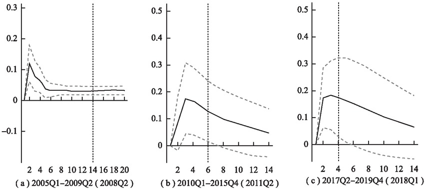
Figure 2 shows the impulse response results of the aggregate output factors in the three complete theoretical cycles in the sample period under a unit-positive MP shock with monetary policy quantity index. It can be seen from Figure 2 that under the effect of one unit of expansionary monetary policy, the output shows a rapidly rising tendency in a theoretical cycle in whatever cyclical period. It is consistent with the economic theory. Meanwhile, all the three figures show that the effects of monetary policy shocks have reached their maximum before the 5th quarter (the 4th, the 3rd and the 5th quarters), with intensities of regulation [1] of 0.07, 0.06 and 0.04, respectively, indicating that the short-term regulations of expansionary monetary policy on output is effective. However, in whatever cycle, after 10 quarters, all outputs basically converge to the steady-state level of 0, and the output in Figure 2 (c) slightly exceeds the steady-state level with a very small magnitude. The monetary policy effects disappear completely after about 20 quarters. Figure 3 shows the identification results based on policy cycle in cross-cycle adjustment, presenting in two policy cycles in the three figures the impulse response results of output factors under the positive monetary policy shocks. It can be seen in Figure 3 that the policy cycle is relatively short compared with the theoretical cycle, the monetary policy shocks tend to converge within a policy cycle (2011Q4–2015Q4) in only one impulse response figure, while the other two impulse responses reach the peak value in the first cycle (2009Q3–2011Q3, 2016Q1–2018Q1). All the impulse responses have lasted to the second cycle (2011Q3–2015Q4, 2018Q1–2019Q4) before returning to the steady-state point. In addition, both Figure 3 (a) and Figure 3 (c) show expansionary monetary policy, and are manifested as counter-cyclical adjustments in two cycles. The impulse response results may indicate that the division characteristics of policy cycle with mutation points as boundaries and the economic characteristic differences in different cycles are important reasons for the differences in cross-cycle adjustment effects between the “theoretical cycle” and the “policy cycle”.

Impulse Responses of Aggregate Output to Monetary Policy Shocks Based on Theoretical Cycle Division
Note: The time interval spans two cycles, which are delimited by broken lines, and what in the parentheses are the time points of cross-cycle delimitation.

Impulse Responses of Aggregate Output to Monetary Policy Shocks Based on Policy Cycle Division
4 Further Analyses
4.1 Industrial Output
An important fact about cyclical volatility is that the fluctuation degrees of different components of output vary. As a leading sector of the national economy, industry is most related to the real estate industry and the manufacturing industry, the change of industrial added value indicates that of corporate profits, and the decline of the value means reduction of corporate profits and the change of the tendency of economic fluctuations. It shows that the cross-cycle adjustment effects of monetary policy on industrial output matter directly to how to increase the effects of aggregate output cross-cycle adjustment. According to this, in this section, we will discuss whether monetary policy has cross-cycle adjustment effects on industrial output, with industrial added value as an industrial output indicator. After taking a logarithm of the industrial added value, we use the HP filtering method to obtain the component of fluctuation, and then use the trend mutation method to divide the policy cycles of industrial output, and the division results are shown in Figure 4. The result shows that except for a few economic shock events which make shocks on industrial output one quarter earlier, the policy cycle division result of industrial output is basically consistent with that of aggregate output.

Policy Cycle Variation Tendency of Industrial Output
Figure 5 shows the impulse response results of industrial output based on different policy cycles under one unit standard deviation monetary policy shock, with industrial output factor module added to the FAVAR model. It can be seen in Figure 5 that, within the range of any policy cycle, monetary policy shocks tend to converge rapidly within a single cycle, their effects are stronger and last shorter than those of aggregate output (the intensity of regulation is 0.06, 0.04, 0.11 and 0.05, respectively), and there are no effects of cross-cycle adjustment.

Impulse Responses of Industrial Output to Monetary Policy Shocks
As is seen from the above results, the aggregate output that has been smoothed out has stronger persistence than industrial output under the monetary policy shocks. Through comparative analyses, we believe that there are two potential causes for the differences. First, compared with aggregate output, industrial output is more likely to be influenced by expectations and are more sensitive to economic uncertainties, while the components such as consumption and government expenditures in aggregate output are relatively stable. Second, the changes of aggregate output indicators are smoother than those of structural output indicators, which is manifested by the fact that the persistence of aggregate output indicators is longer under the positive of monetary policy shocks, exhibiting the function of cross-cycle adjustment to a certain extent.
But for industrial output, although the policy has greater effects, its sustainability is poorer and the cross-cycle adjustment effects are limited. The above results show that, the effects of monetary policy cross-cycle adjustment are mostly achieved through the joint effects on components of aggregate output. It helps enhance monetary policy cross-cycle adjustment effects by differentiating the regulations of monetary policy on the components of the output structure in a targeted manner.
4.2 Degree of Economic Uncertainty
When the uncertainties the macro economy faces increase, it is more difficult for the People’s Bank of China to develop expectations for the future, directly affecting the effects of monetary policy regulation. Accordingly, in this section we further discuss about the causes of and possible countermeasures for the differences in monetary policy cross-cycle adjustment effects from the perspective degree of economic uncertainty.
As for indicators for measuring the degree of economic uncertainty, different methods are used in existing researches. Here, we use the practices of Talavera et al.( (2012) as reference and adopt the conditional variance of seasonal actual GDP change rates measured by the GARCH (1, 1) model as the indicator for measuring the degree of macroeconomic uncertainty. On the basis of the degree of economic uncertainty, we conduct interval division on policy cycle on the basis of the three-stage division of cyclical volatility, as is shown in Table 4.
Interval Division and Degree of Uncertainty of Economic Cyclical Volatility
| Growth stage |
Stationary stage |
Recession stage |
|||
|---|---|---|---|---|---|
| Duration interval | Uncertainty index | Duration interval | Uncertainty index | Duration interval | Uncertainty index |
| 2000Q1–2000Q4(4) | 2.08 | 2001Q1–2001Q3(3) | 1.54 | 2001Q4–2003Q2(7) | 3.64 |
| 2003Q3–2004Q4(6) | 11.48 | 2005Q1–2008Q2(14) | 12.43 | 2008Q3–2009Q3(5) | 43.29 |
| 2009Q4 (1) | 5.80 | 2010Q1–2011Q2(6) | 1.48 | 2011Q3–2015Q4(18) | 18.22 |
| 2016Q1–2017Q1(5) | 2.08 | 2017Q2–2018Q1(4) | 1.89 | 2018Q2–2020Q1 (8) | 4.50 |
| 2020Q2–2021Q1(4) | 122.00 | 2021Q2(1) | 40.88 | 2021Q3–2021Q4(2) | 143.70 |
It can be seen from the interval division results that the stage with a higher degree of economic uncertainty basically coincides with economic recession stage, while the stage with a lower degree of economic uncertainty coincides with stationary stage in each economic cycle. According to the above internal divisions, we divide the existing policy cycles into stationary fluctuation stage (economic stationary stage) and accelerated fluctuation stage (economic recession stage), and apply one unit standard deviation monetary policy shock on the aggregate output in the three stationary stages. The impulse response results in Figure 6 shows that, in the stage with a lower degree of economic uncertainty, the impulse responses of aggregate output generally cross the cyclic demarcation point. They feature slow and persistent convergence, gradually converge to the level before the shocks after crossing the cyclic demarcation point, and there are cross-cycle adjustment effects; while in the stage with a higher degree of economic uncertainty, one unit standard deviation monetary policy shock can not achieve cross-cycle adjustment as in all time frames monetary policy shocks converge to the steady-state level at zero within a single cycle. Further, for the period with a higher degree of economic uncertainty, we use the practices of Chen and Liu (2012), and Zhou and Zhao (2016) for reference and further investigate the regulation effects of monetary policy on output by increasing the intensity of monetary policy shocks. The results in Figure 7 show that, when the monetary policy shock increases from one unit standard deviation to two unit standard deviations, the intensity of regulation increases, the fluctuation magnitude of output rises, the sustainability of shock improves obviously, and impulse responses generally approach to 0 in the next cycle.
Impulse Responses of Output to Monetary Policy Shocks in the Stationary Fluctuation Stage

Impulse Responses of Output to Monetary Policy Shocks in the Accelerated Fluctuation Stage
The above results indicate that the severer the negative shock on the economy, the worse the effects of cross-cycle policy adjustment, it is inconsistent with the policy intention of strengthening cross-cycle policy adjustment in the period of economic downturn, indicating that perhaps we should reconsider how to seize the opportunities for cross-cycle policy adjustment. Nevertheless, our research results also show that though excessively great monetary policy regulation may cause economic fluctuations in the next cycle, the implementation of more proactive monetary policy in a period with higher degree of economic uncertainty is likely to increase its cross-cycle adjustment effects.
4.3 Monetary Policy Stance and Tools
When the economy enters the growth stage, the People’s Bank of China usually adopts a tight monetary policy on counter-cyclical adjustment in order to prevent extensive credit expansion; when the economy enters the recession stage, the People’s Bank of China is more likely to adopt expansionary monetary policy. However, since there are higher stickness in reduction of price and nominal wages in economy, it is generally believed that tight monetary policy will generate more shocks compared with expansionary monetary policy. Therefore, the asymmetric effects of monetary policy stance may also affect the cross-cycle adjustment effects of the policy. In addition, the action mechanisms and effects of different types of monetary policy tools vary in the case of different monetary policy stances. As for China’s specific circumstances, some researches consider that if tight monetary policy is used to address the issue of economic overheating, then there is little difference between the effects of quantity-based monetary policy and those of price-based monetary policy. Some researches suggest that price-based monetary policy is more effective for stimulating output growth in the period of economic depression; however, in the economic growth stage, if it aims to smooth out the output fluctuations, a quantity-based monetary policy shall be adopted (Zhang and Jin, 2018). In recent years, establishing an effective interest rate regulation system has become the main goal of China’s transformation of monetary policy rules. Therefore, in this section, we take 7-day inter-bank interest rate as price-based monetary policy indicator and replace M2 growth rate as the monetary policy factor in the FAVAR model of Formula (3), so as to use different policy tools to find out the differences in cross-cycle adjustment effects that may exist in different monetary policy stances.
In most periods of economic recession (2008Q3, 2016Q1), the People’s Bank of China implemented expansionary monetary policy on counter-cyclical adjustment, however, in all periods of economic growth except for 2020Q3, the People’s Bank of China generally implemented tight monetary policy[1] (2005Q2, 2011Q2). Accordingly, we make one unit standard deviation quantity-based monetary policy shock on the aggregate output in the above periods. The results are shown in Figure 8 and Figure 9. Of which, Figure 8 shows that cross-cycle adjustment effects have been achieved under the expansionary monetary policy shocks, and are manifested as countercyclical adjustment in the next cycle, the maximum intensities of regulation are 0.063 and 0.033, and all impulse responses gradually converge to 0 in the next cycle. Figure 9 shows that in the economic growth stage, if one unit standard deviation monetary policy shock has been made, the effect of tight monetary policy shock will reach the maximum value before the 3rd quarter, their intensities of regulation are about 0.09 and 0.06, it reaches its peak value faster than expansionary monetary policy, but converges rapidly later on, and there are not cross-cycle adjustment effects at all.

Impulse Responses to the Quantity-Based Tool Shocks in the Economic Recession Stage

Impulse Responses to the Quantity-Based Tool Shocks in the Economic Growth Stage
The impulse response results with added price-based monetary policy indicators are shown in Figure 10 and Figure 11, and one unit standard deviation monetary policy shock can cause negative response of output. It can be seen from Figure 10 that in the economic recession stage the effect of the monetary policy shock will reach its maximum before the 5th quarter, the greatest intensity of regulation is 0.06, impulse responses gradually converge after crossing the dividing line of the policy cycle, generating cross-cycle adjustment effects. The persistence of shocks increased significantly after 2016, which is likely to be related to deregulation of deposit interest rates after 2015Q4. It can be seen from Figure 11 that, in the economic growth stage, impulse responses caused by one unit standard deviation price-based monetary policy shock generally reach their maximum before the 4th quarter, the intensity of regulation is about 0.05, slightly lower than the intensity of the price-based monetary policy shock in the economic recession stage. In addition, the impulse responses in the economic growth stage persist shorter than in the economic recession stage, converge to the level before the shock before the 9th quarter, and there are no cross-cycle adjustment effects.

Impulse Responses to the Price-Based Tool Shocks in the Economic Recession Stage

Impulse Responses to the Price-Based Tool Shocks in the Economic Growth Stage
By comparing the impulse responses of the two types of monetary policy tools to output, we can find that, in the economic recession stage, both the impulse responses have cross-cycle adjustment effects, but the impulse response of quantity-based monetary policy shocks to output is greater than that of price-based monetary policy shocks no matter in terms of intensity or length of time, the impulse responses converge to 0 after the 11th quarters, and the greatest intensity of regulation is 0.063, significantly higher than that of price-based monetary policy tools. In the economic growth stage, both quantity-based and price-based monetary policy tools have no cross-cycle adjustment effects, the quantity-based monetary policy tools are slightly greater than price-based monetary policy tools in terms of intensity, while price-based monetary policy tools are slightly greater than quantity-based monetary policy tools in terms of persistence. This shows that, though the cross-cycle adjustment effect of price-based monetary policy and that of quantity-based monetary policy are basically consistent with each other no matter in economic recession stage and economic growth stage, but the cross-cycle adjustment effect of price-based monetary policy is worse than that of quantity-based monetary policy in economic recession stage no matter in persistence and intensity, in line with the consensus that the stimulation effect of quantity-based monetary policy is better than that of price-based monetary policy in the economic recession stage, but the result does not conform with the research results of Zhang and Jin (2018), and Bian and Hu (2015), and the reason for this is that the degrees of interest rate liberalization vary in different research periods.
4.4 Expected Effects
Monetary policy expectation management, namely the decision-making authority adopts feasible policies or measures to guide market expectations for achieving monetary policy goals such as output increase, etc. (Wang and Wang, 2021). Although the important influence of expectation management on the effects of monetary policy implementation has been widely accepted at home and abroad, existing researches on monetary policy expectations usually pay attention to market expectations for the implementation of monetary policy of the People’s Bank of China, and focus mainly on differentiated impacts of expected and unexpected monetary policies on the economy (Wang et al., 2016; Zhuang et al., 2018). Different from market expectations in existing literature, similar to forward-looking monetary policy, which introduces cyclical factors into monetary policy rules so as to avoid possible problem of sunspot multiple equilibria, the expectation this paper focuses on refers to the expectation of the People’s Bank of China for the future value of the variable that it is concerned about, while the expected effect refers the effect of fact that the People’s Bank of China includes the expectation of the future value of the variable it is concerned about into the decision-making information set on the realization of monetary policy cross-cycle adjustment. Therefore, different from the measurement thought in most previous literature on of separation between expected monetary policy and unexpected monetary policy (Guo et al., 2016; Zhu and Zhou, 2018), we assume that the monetary policy information set of the People’s Bank of China contains expectations for future outputs, use the practice of Zhang and Zhang (2007) as reference, include the previous aggregate output module into the FAVAR model of Formula (3), so as to judge whether the inclusion of the expected value of the variable that the People’s Bank of China is concerned about have a positive impact on the effects of monetary policy cross-cycle adjustment.
The impulse response results containing expectations (see Figure 12 and Figure 13) show that, no matter in the economic recession stage or the economic growth stage, the effect of one unit monetary policy shock on output is greater than that of monetary policy shock that contains no expectation in terms of intensity of regulation and time characteristics. Specifically, in the economic recession stage, under one unit expansionary monetary policy shock, output responses generally reach the peak value in the 5th quarter, the minimum intensity of regulation is 0.064, significantly greater than the maximum intensity of regulation 0.052 in the case that expectations are not included. In addition, the continuity of impulse effects also increases noticeably. In the economic growth stage, the effect of tight monetary policy with expectations is obviously higher than the effect of monetary policy without expectation, of which impulse responses generally reach the maximum value before the 4th quarter, the continuity of impulse responses is longer than that of monetary policy without expectations, and cross-cycle adjustment effects increase significantly. This shows that, if the expectation of the People’s Bank of China has been included, it is easier for both expansionary monetary policy and tight monetary policy to achieve cross-cycle adjustment effects, and both the intensity and persistence of policy improve, being in stark contrast to the effect of monetary policy containing no expectation. It also indicates that cross-cycle adjustment can be regarded as a kind of policy design variant of expected monetary policy regulation in the environment with higher degree of uncertainty, and reinforcing expectations is still the key to cross-cycle adjustment.

Impulse Responses of Output to Monetary Policy Shocks Containing Expectation in the Economic Recession Stage

Impulse Responses of Output to Monetary Policy Shocks Containing Expectation in the Economic Growth Stage
5 Conclusions and Policy Implications
To address the problem that standard monetary policy theory can hardly explain the cross-cycle adjustment function of monetary policy, this paper, on the basis of cyclic delimitation of the monetary policy cross-cycle adjustment, identifies and measures China’s macroeconomic cycles, compares monetary policy cross-cycle adjustment effects in different circumstances, makes a systematic analysis of whether China’s monetary policy has cross-cycle adjustment effects and what kind of policy operation is more helpful for achieving the goal of cross-cycle adjustment, and has made some inspiring conclusions and policy implications.
First, the effects of monetary policy cross-cycle adjustment are generally limited, have relatively strong state dependence, and are closely related to the timing for policy operation and the duration of cycle. The empirical results of this paper show that, monetary policy based on “theoretical cycle” has no cross-cycle adjustment effects on aggregate output, but “policy cycle” based on policy implications has certain cross-cycle adjustment effects. As for aggregate output, though cross-cycle policy adjustment has some effects initially, these effects will rapidly decline over time, and the continuity of monetary policy effects varies in different stages. Further studies show that monetary policy has no cross-cycle adjustment effects on industrial output, and monetary policy cross-cycle adjustment effects are related to the degree of economic uncertainty. Cross-cycle policy adjustment effects in a period with a lower degree of economic uncertainty are significantly better than those in a period with higher degree of economic uncertainty, however, as policy regulation is intensified against the increasing degree of economic uncertainty, the cross-cycle adjustment effects will be enhanced to a certain extent.
Second, monetary policy cross-cycle adjustment effects are related to monetary policy stance and tools. According to empirical results, in the economic recession stage, the implementation of expansionary monetary policy by using quantity-based monetary policy tools is more helpful for achieving cross-cycle adjustment; in the case of implementation of tight monetary policy in the economic growth stage, cross-cycle adjustment effects do not exist no matter quantity-based monetary policy or price-based monetary policy is adopted, this is consistent with the judgment of western countries about monetary policy effects but differs from the research conclusions of Chinese scholars, due to the possible reason that the degrees of interest rate liberalization differ in the research interval.
Third, monetary policy cross-cycle adjustment effects are closely related to whether expectation factors are considered and increase noticeably after expectation factors are included. This implies that monetary policy cross-cycle adjustment is very likely a special form of forward-looking monetary policy, so we need to follow the basic rules of forward-looking monetary policy and solve the particular problems of forward-looking monetary policy.
Last, the research in this paper has relatively important policy implications. Currently, the shocks of external uncertainties significantly intensify, extending short-term policy to mid- and long-term policies. Properly handling the dialectical relationships between the “status” and the “trend” of economic cycle and promoting monetary policy cross-cycle design and adjustment are important ways for promoting recovery and steady development of China’s economy and boosting high-quality development, and it is also a concrete practice of fulfilling the requirements on “improve the macroeconomic governance system” stated in the report to the 20th CPC National Congress. The research in this paper also indicates that monetary policy cross-cycle adjustment effects are not only closely related to conformity to forward-looking rules and the timing of policy, but also related to frequency of economic cyclical volatility, the intensity of regulation in different economic situations and the selection of monetary policy stance and tools. To increase the effectiveness of monetary policy cross-cycle adjustment, we need to reinforce monetary policy expectations under the precondition of following monetary policy forward-looking rules, ensure a proper intensity of monetary policy regulation in accordance with the degree of economic uncertainty, make flexible use of quantity-based monetary policy and price-based monetary policy under different economic circumstances, further increase the level of interest rate liberalization, improve the interest rate channel transmission mechanism, and increase the stability and sustainability of monetary policy regulation.
References
Bernanke, B., Boivin, J., & Eliasz, P. (2005). Measuring Monetary Policy: A Factor Augmented Vector Autoregressive (FAVAR) Approach. Quarterly Journal of Economics, 120(5), 387–422.10.1162/qjec.2005.120.1.387Suche in Google Scholar
Bian, Z., & Hu, H. (2015). China’s Selection of Monetary Policy Tools: Quantity-Based or Price-Based?—An Analysis Based on the DSGE Model. Studies of International Finance (Guoji Jinrong Yanjiu), 6, 12–20.Suche in Google Scholar
Chan, K. (1990). Testing for Threshold Autoregression. The Annals of Statistics, 18(4), 1886–1894.10.1214/aos/1176347886Suche in Google Scholar
Chen, K. J., Ren, J., & Zha, T. (2018). The Nexus of Monetary Policy and Shadow Banking in China. American Economy Review, 108(12), 3891–3936.10.1257/aer.20170133Suche in Google Scholar
Chen, L., & Liu, Y. (2012). Empirical Researches on the Nonlinear Effects of Net Export Demands of China’s Monetary Policy under Different Exchange Rate Regimes. Studies of International Finance (Guoji Jinrong Yanjiu), 12, 4–11.Suche in Google Scholar
Chen, X., Liu, L., & Chen, Y. (2022). The Overall Logic for Innovating and Improving Macro Control: From the Perspective of the “Three-in-One” Macro Police. Reform (Gaige), 3, 10–23.Suche in Google Scholar
Cheng, J., Li, X., & Liu, X. (2015). A Study on the Heterogeneity of Inflation Expectations in China and Inflation Expectation Management of China’s Central Bank. Economic Research Journal (Jingji Yanjiu), 6, 17–39+54.Suche in Google Scholar
Fan, C., Sheng, T., & Wang, Y. (2012). A Study on the Term Structure of Economic Effects of Credit Volume. Economic Research Journal (Jingji Yanjiu), 1, 80–91.Suche in Google Scholar
Galí, J. (2015). Monetary Policy, Inflation, and the Business Cycle: An Introduction to the New Keynesian Framework and Its Applications. Princeton: Princeton University Press.Suche in Google Scholar
Guo, Y., Huang, Z., & Wang, Y. (2016). Unexpected Monetary Policy and Corporate Bond Credit Spread: A Study on Decomposition of Fixed and Floating Interest Rate Spreads. Journal of Financial Research (Jinrong Yanjiu), 6, 67–80.Suche in Google Scholar
Guo, Y., Chen, W., & Chen, Y. (2016). A Study on the Decline of Effectiveness of China’s Monetary Policy and Expectation Management. Economic Research Journal (Jingji Yanjiu), 1, 28–41+83.Suche in Google Scholar
Krueger, A. (1993). Virtuous and Vicious Circles in Economic Development. American Economic Review, 83(2), 351–355.Suche in Google Scholar
Kydland, F., & Prescott, E. (1977). Rules Rather than Discretion: The Inconsistency of Optimal Plans. Journal of Political Economy, 85(3), 473–491.10.1086/260580Suche in Google Scholar
Li, H. (2012). The Predictive Effects of the Term Structure of Interest Rate on Forward Interest Rate—Test of the Expectation Hypothesis Modified via Term Premium. Journal of Financial Research (Jinrong Yanjiu), 8, 97–110.Suche in Google Scholar
Liu, J., & Zheng, T. (2008). The Division of Periodic Division of China’s Economic Cycle and Analyses on Economic Growth Trends. China Industrial Economics (Zhongguo Gongye Jingji), 1, 32–39.Suche in Google Scholar
Ma, L., He, M., & Liu, Y. (2016). A Study on Monetary Policy Transmission Based on Adaptive Expectations. Journal of Financial Research (Jinrong Yanjiu), 8, 19–33.Suche in Google Scholar
Ma, W. (2014). Global Inflation Expectation Management: Historical Experience and Practical Enlightenment. The Journal of Quantitative & Technical Economics (Shuliang Jingji Jishu Jingji Yanjiu), 11, 86–102.Suche in Google Scholar
Romer, D. (2019). Advance Macroeconomics (Fifth Edition). New York: McGraw-Hill Education Press.Suche in Google Scholar
Sinha, A. (2015). FOMC Forward Guidance and Investor Beliefs. American Economic Review, 105(5), 656–661.10.1257/aer.p20151123Suche in Google Scholar
Talavera, O., Tsapin, A., & Zholud, O. (2012). Macroeconomic Uncertainty and Bank Lending: The Case of Ukraine. Economic Systems, 36(2), 279–293.10.1016/j.ecosys.2011.06.005Suche in Google Scholar
Tan, X., & Zhang, W. (2017). An Analysis on the Channels via Which Economic Policy Uncertainties Affect Enterprise Investment. The Journal of World Economy (Shijie Jingji), 12, 3–26.Suche in Google Scholar
Wang, X., & Wang, X. (2021). A Study on Strategies for Improving Monetary Policy Expectation Management. Finance & Trade Economics (Caimao Jingji), 2, 67–85.Suche in Google Scholar
Wang, X., Wang, X., & Chen, Z. (2016). Monetary Policy Expectations and Inflation Management—DSGE Analysis Based on Message Shock. Economic Research Journal (Jingji Yanjiu), 2, 870–893.Suche in Google Scholar
Wang, Y., Wang, Y., & Yang, H. (2021). Types of External Shocks and China’s Economic Cyclical Volatility—On the Effectiveness of Prudent Macro Policies. Studies of International Finance (Guoji Jinrong Yanjiu), 3, 14–26.Suche in Google Scholar
Woodford, M. (1990). Learning to Believe in Sunspots. Econometrica: Journal of the Econometric Society, 58, 2, 277–307.10.2307/2938205Suche in Google Scholar
Zhang, L., & Jin, C. (2018). A Comparative Study on the Effectiveness of Quantity-Based and Price-Based Monetary Policy Tools. China Industrial Economics (Zhongguo Gongye Jingji), 1, 119–136.Suche in Google Scholar
Zhang, X. (2021). Macro Leverage Ratio and Cross-Cycle Adjustment. China Finance (Zhongguo Jinrong), 5, 58–60.Suche in Google Scholar
Zhang, Y., & Zhang, D. (2007). The Test of Forward-Looking Monetary Policy Response Function in China’s Monetary Policy. Economic Research Journal (Jingji Yanjiu), 3, 20–32.Suche in Google Scholar
Zhou, J., & Zhao, L. (2016). RMB Exchange Rate Fluctuation and Difficulties in Monetary Policy Regulation. Journal of Finance and Economics (Caijing Yanjiu), 2, 85–96.Suche in Google Scholar
Zhu, X., & Zhou, L. (2018). Unexpected Monetary Policy and Stock Market—An Empirical Study Based on Media Data. Journal of Financial Research (Jinrong Yanjiu), 1, 102–120.Suche in Google Scholar
Zhuang, Z., Jia, H., & Liu, D. (2018). A Study on the Macroeconomic Effects of Monetary Policy: From the Perspectives of Expected and Unexpected Shocks. China Industrial Economics (Zhongguo Gongye Jingji), 7, 80–97.Suche in Google Scholar
© 2023 Minghua Zhan, Yao Lu, Published by DeGryuter
This work is licensed under the Creative Commons Attribution 4.0 International License.
Artikel in diesem Heft
- Frontmatter
- Is There Cross-Cycle Adjustment in China’s Monetary Policy?
- Local Government Debt, Sectoral Linkage and Resource Allocation Efficiency
- VAT Neutrality and Corporate Cash Holdings —Based on the Research of Uncredited VAT Refund Policy
- Unintended Results: Inter-Provincial Differences in Environmental Protection Tax Rates and Relocation Strategies of Polluting Enterprises
- The Size of Individual Social Networks and Rural-Urban Migrants’ Wages—Findings from a Survey of Migrants in China’s 6 Provinces and 12 Cities
- Leading High-Quality Development of Service Industry with Institutional Innovation