
On the Choice of Liability Rules
-
Rajendra P. Kundu

 and
Debabrata Pal
and
Debabrata Pal

Abstract
Legal assignment of liabilities for losses arising out of interactions involving negative externalities usually depend on which of the interacting parties are negligent and which are not. It has been established in the literature that, if negligence is defined as failure to take some cost-justified precaution then there is no liability rule which can always lead to an efficient outcome. The objective of this paper is to try and understand if it is still possible to make pairwise comparisons between rules on the basis of efficiency and to use such a method to explain/evaluate choices from a given set of rules. We focus on a set of five of the most widely analyzed rules (no liability, strict liability, negligence, negligence with the defense of contributory negligence and strict liability with the defense of contributory negligence), and use a binary relation according to which a rule in the set is considered to be at least as efficient as another if and only if the set of applications for which it is inefficient is a subset of the set of applications for which the other one is inefficient. We show that, with respect to the above mentioned relation, pairwise comparisons between rules in this set fail. The paper, thus, demonstrates that an efficiency based explanation for any choice from these five rules is not consistent with the notion of negligence defined as failure to take some cost-justified precaution.
1 Introduction
Courts from across the world are routinely required to decide on matters relating to apportionment of losses resulting from accidents. A variety of rules are used by courts for the assignment of liabilities for such losses. Which of these rules, by providing appropriate incentives to parties involved, always results in efficient outcomes is a key question addressed in economic analysis of law.[1] The attempt here is to examine whether an efficiency based explanation can be provided for why some rules are (ought to be) chosen over others.
In the standard framework,[2] the question is analysed in the context of interactions between two risk-neutral parties who are strangers to one another. It is assumed that the loss, in case of accident, falls on one of the parties called the victim. The other party is referred to as the injurer. The probability of accident and the actual loss in case of accident are assumed to depend on the care levels of the two parties. It is also assumed that, the social objective is to minimize the total social costs which are defined as the sum of costs of care of the parties involved and the expected accidental loss. The assignment of liabilities for accidental losses by courts is usually based on the levels of nonnegligence of the victim and the injurer where the level of nonnegligence of a party is either 0 (indicating that the party is negligent) or 1 (indicating that the party is nonnegligent). A rule for the assignment of liabilities specifies the proportions of the loss, in case of occurrence of accident, that the victim and the injurer have to bear for every possible combination of their levels of nonnegligence.
It is assumed that, parties have common knowledge about their interaction (the rule, the possible care levels for both with their corresponding costs and the expected accident losses) and choose their respective care levels simultaneously to minimize their expected costs where the expected cost of a party is the sum of cost of her chosen care level and the expected value of her share of the loss. Thus, an interaction between the parties is modeled as a static game of complete information. A rule for assignment of liabilities is said to be efficient if and only if it always induces both parties to choose care levels that minimize total social costs.
Since the apportionment of accidental losses by courts is usually based on who is negligent and who is not, determination of negligence of a party involved in an accident is a very crucial element of the process of liability assignment and can have important implications. In the standard literature on the efficiency of rules for the assignment of liabilities for accidental losses, negligence is usually defined as a shortfall from a court-specified total social cost minimizing due care level.[3] Thus, an injurer (victim) is considered negligent if and only if she is found to have taken less than the care due from her. Negligence has, alternatively, been defined as the failure to take a cost-justified precaution.[4] Given the care levels of the two parties, any other care level of a party (which is higher than her actual care) is cost-justified if and only if it involves an additional cost which is less than the reduction in expected loss it would have brought about. Thus, according to this notion, injurer (victim) is considered negligent if and only if the other party can demonstrate a failure on her part to take some cost-justified precaution.
It has been established in the literature that, if negligence is defined as shortfall from legally specified total social cost minimizing due care then there are liability rules which provide appropriate incentives for taking efficient levels of care to involved parties.[5] It has also been established that no rule is efficient when negligence is defined as failure to take some cost-justified precaution.[6] Thus, while the notion of negligence as shortfall from due care is consistent with the objective of efficiency, the notion of negligence as failure to take some cost-justified precaution is not.
The existence of cost-justified untaken precaution approach to determination of negligence, though inconsistent with the objective of efficiency, has several advantages to its credit. The determination of negligence according to the shortfall from due care approach requires the court to play an active role in collecting and processing information on costs of care of parties and expected accident losses. In the other approach, while the injurer (victim) has to demonstrate the existence of some cost-justified untaken precaution of the victim (injurer) to establish her negligence, the court plays the role of a neutral referee. Thus, in comparison to the shortfall from due care approach, this approach is more in harmony with the adversarial system of law. It has been argued that, the cost of determining efficient level of care by courts can be significantly more than the costs that parties might have to incur in establishing negligence of each other. It has also been argued that, in determining negligence, courts actually do not try to fix due care levels but look for evidence of failure to take a cost-justified precaution.[7] It is, therefore, important to explore the possibility of retaining efficiency considerations in the standard model while using the notion of negligence as failure to take some precaution which is cost-justified.
In this paper, we pose the following question: if negligence is defined as the existence of some cost-justified untaken precaution then is it possible to choose a rule from a given set on the basis of efficiency considerations? To answer the above question we define a binary relation on a set of rules as follows: a rule is at least as efficient as another if and only if the set of applications for which it is inefficient is a subset of the set of applications for which the other one is inefficient. Accordingly, a rule is said to be more efficient than another if and only if the set of applications for which it is inefficient is a proper subset of the set of applications for which the other one is inefficient. A rule in the set is best if and only if it is at least as efficient as every other rule in the set. A rule in the set is maximal if and only if there is no other rule in the set which is more efficient. If there exists a rule which is best in the set with respect to the above relation then such a rule is an obvious choice. If no rule is best but some rule is maximal in the set then such a rule is socially desirable. In this paper, we focus on the set of the following five rules which are among the most widely used and also the ones most analysed in the literature: no liability, strict liability, negligence, negligence with the defense of contributory negligence and strict liability with the defense of contributory negligence.[8] It turns out that, none of these rules is comparable to any of the others and therefore none is best but every rule is maximal with respect to the above relation. Thus, it follows that, when negligence is defined as the existence of some cost-justified untaken precaution, it is not possible to make a meaningful choice from these five rules on the basis of efficiency considerations as embedded in the relation discussed above.
The paper is organized as follows: The model is presented in Section 2. All definitions and assumptions are stated here and are illustrated with appropriate examples. Section 3 states an impossibility result. Section 4 presents the main results of the paper in the form of Theorems 1 and 2 and also contains the intermediate results (Lemmas 1–5) which are used to prove the two theorems. Section 5 concludes the paper with a discussion on the implications of the results.
2 Model
We consider interactions between two parties (generically called party i, where
We denote by
We also assume that
In view of (A2) and (A3) it follows that
Let
We assume:
(A4) implies that L is non-increasing in
We define the total social cost of the interaction between the two parties,
Let
2.1 Negligence as Failure to Take Some Cost-justified Precaution
Consider any
Let
Thus,
At
2.2 Simple Liability Rule
A simple liability rule is a function
Example 1.
Consider the following simple liability rules:
Rule of no liability
Rule of strict liability
Negligence rule (
Negligence rule with the defense of contributory negligence (
Rule of strict liability with the defense of contributory negligence (
A rule for the assignment of liabilities can be more generally formalized as a liability rule. A liability rule is a function
Remark 1.
Corresponding to every simple liability rule g there is a class of liability rules
Example 2.
Consider the following liability rule:
Rule of comparative negligence (
Note that
However, the assignment of liabilities under
2.3 Application of a Rule
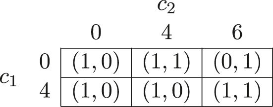
An application, ω, is a specification of
Let g be any simple liability rule and
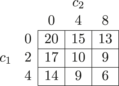
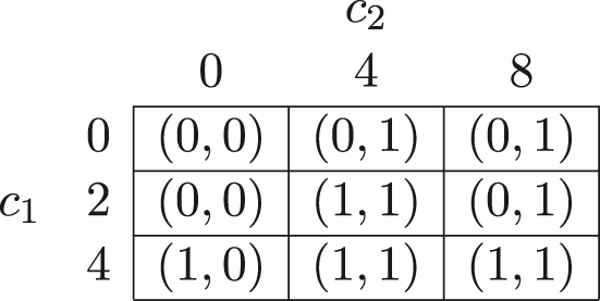
Example 3.
Let
Application
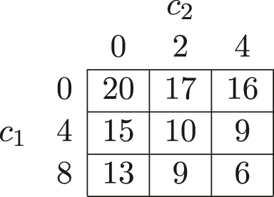
|
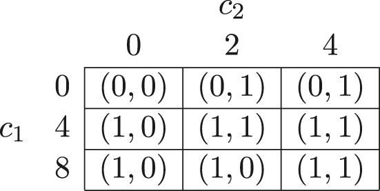
|
Note that
2.4 Efficiency
A simple liability rule, g, is said to be efficient for ω iff (i)
Remark 2.
Note that, if
Let
Remark 3.
It is clear that, (i) if g and
3 Negligence as Failure to Take Some Cost-justified Precaution and the Efficiency of Simple Liability Rules: An Impossibility
In this section we analyse efficiency properties of simple liability rules with negligence defined as the existence of some cost-justified untaken precaution. The main result here establishes that, if negligence is defined as failure to take some cost-justified precaution then no simple liability rule can always achieve an efficient outcome. The result is stated as Proposition 1 given below:
Proposition 1.
If negligence is defined as failure to take some cost-justified precaution then no simple liability rule is efficient for
In view of Remarks 1 and 2 it is immediate that Proposition 1 follows as a corollary to Theorem 1 of Jain (2006) which states that, if negligence is defined as failure to take some cost-justified precaution then there is no liability rule which is efficient for
4 Choice of Rules when Negligence Is Defined as Failure to Take Some Cost-justified Precaution
In this section we focus on,
Lemma 1 states that there is no rule in
Lemma 1.
Proof.
Let
Application
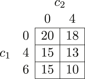
|
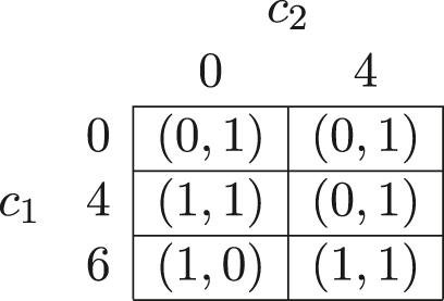
|
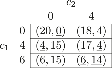
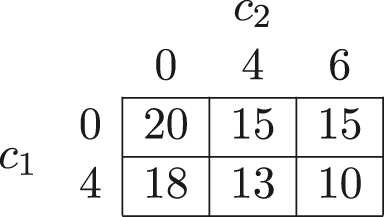
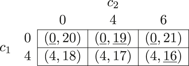
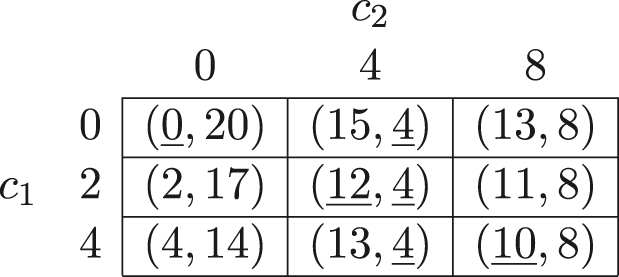
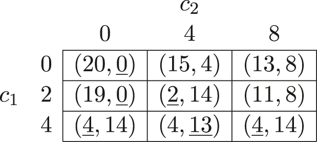
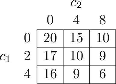
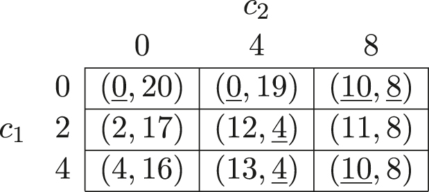
Table 4.2 is the
Payoff matrix for
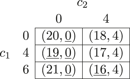
|
Payoff matrix for
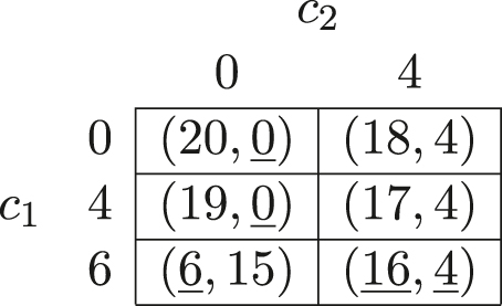
|
(6, 4)
As there is no configuration of costs at which the victim and the injurer are both negligent,
(6, 4) is also the unique Nash equilibrium of
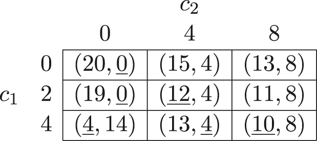
Payoff matrix for
|
(1.1) and (1.2) imply that
Lemma 2.
Proof.
Let
Application
|
|
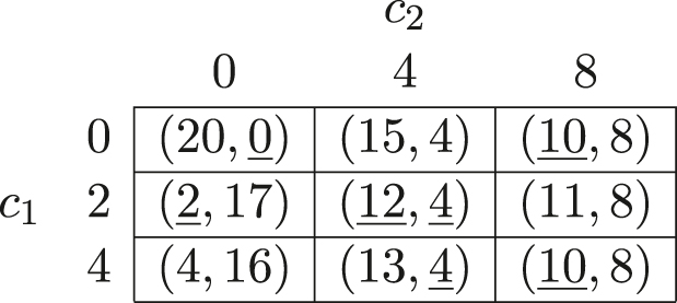
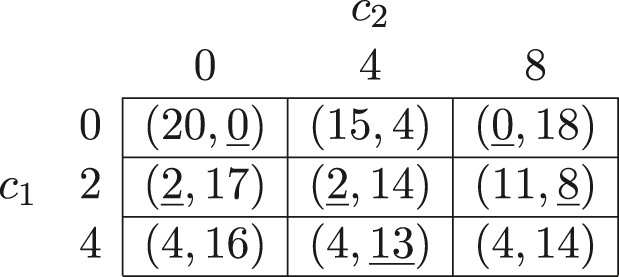
Table 4.7 is the
Payoff matrix for
|
Payoff matrix for
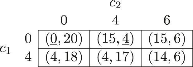
|
Payoff matrix for
|
(4, 6)
As there is no configuration of costs at which the victim and the injurer are both negligent,
(4, 6) is the unique Nash equilibrium of
(2.1) and (2.2) imply that
Lemma 3.
Proof.
Let
Application
|
|
There is no Nash equilibrium in
There is no Nash equilibrium in
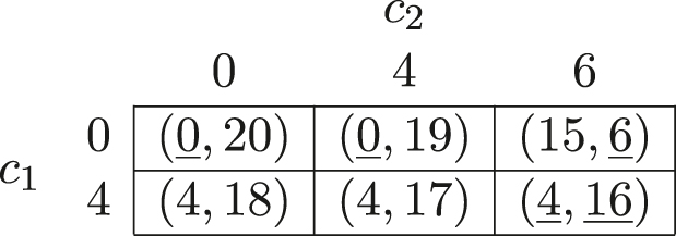
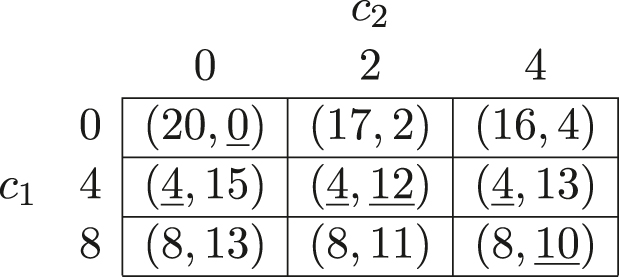
Payoff matrix for
|
Payoff matrix for
|
Payoff matrix for
|
(3.1) and (3.2) imply that
Lemma 4.
Proof.
Let
Application
|
|
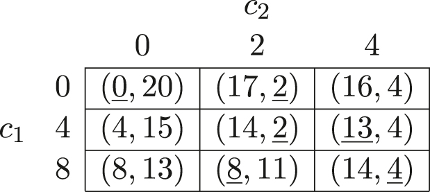
Payoff matrix for
|
Payoff matrix for
|
Payoff matrix for
|
(4.1) and (4.2) imply that
Lemma 5.
Proof.
Let
Payoff matrix for
|
Payoff matrix for
|
Payoff matrix for
|
There is no Nash equilibrium in
There is no Nash equilibrium in
(5.1) and (5.2) imply that
Theorem 1.
Proof.
It follows from Lemmas 1-5 that
Theorem 2.
Proof.
Immediate from Lemmas 1–5.
5 Concluding Remarks
Law and economics as a discipline tries to explain and evaluate laws in terms of economic efficiency. In the context of rules for the assignment of liabilities for accidental losses, while the positive of the law and economics approach has tried to give an efficiency based explanation for adoption of some rules to the exclusion of others, the normative has tried to determine the desirability or otherwise of such rules on the basis of their efficiency properties. In this paper we focus on five of the most widely analysed rules and demonstrate that, if negligence is defined as failure to take some cost-justified precaution then it is not possible to make pairwise comparisons between these rules based on the notion of efficiency to be able to explain why some rules are (ought to be) chosen over the others.
It has to be noted that the results obtained here are restricted to a set of five rules only and it would be interesting to see if the results hold when we extend our analysis to the set of all possible simple liability rules. Further, it has to be noted that the results of the paper are due to the fact that for any pair of rules
References
Brown, J. P. 1973. “Toward an Economic Theory of Liability.” Journal of Legal Studies 2: 323–50. https://doi.org/10.1086/467501.Search in Google Scholar
Calabresi, G. 1961. “Some Thoughts on Risk Distribution and the Law of Torts.” Yale Law Journal 70: 499–553, https://doi.org/10.2307/794261.Search in Google Scholar
Calabresi, G. 1965. “The Decision for Accidents: An Approach to Non-fault Allocation of Costs.” Harvard Law Review 78: 713–45, https://doi.org/10.2307/1338791.Search in Google Scholar
Calabresi, G. 1970. The Costs of Accidents: A Legal and Economic Analysis. New Haven: Yale University Press.Search in Google Scholar
Coase, R. H. 1960. “The Problem of Social Cost.” Journal of Law and Economics 3: 1–44, https://doi.org/10.1086/466560.Search in Google Scholar
Diamond, P. A. 1974. “Accident Law and Resource Allocation.” Bell Journal of Economics 5: 366–405, https://doi.org/10.2307/3003115.Search in Google Scholar
Grady, M. F. 1983. “A New Positive Economic Theory of Negligence.” The Yale Law Journal 92 (5): 799–829, https://doi.org/10.2307/796145.Search in Google Scholar
Grady, M. F. 1984. “Proximate Cause and the Law of Negligence.” Iowa Law Review 69 (1): 363–449.Search in Google Scholar
Grady, M. F. 1989. “Untaken Precautions.” The Journal of Legal Studies 18 (1): 139–56, https://doi.org/10.1086/468143.Search in Google Scholar
Jain, S. K. 2006. “Efficiency of Liability Rules: A Reconsideration.” The Journal of International Trade & Economic Development 15 (3): 359–73, https://doi.org/10.1080/09638190600871685.Search in Google Scholar
Jain, S. K. 2015. Economic Analysis of Liability Rules. India: Springer.10.1007/978-81-322-2029-9Search in Google Scholar
Jain, S. K., and R. Singh. 2002. “Efficient Liability Rules: Complete Characterization.” Journal of Economics (Zeitschrift für Nationalökonomie) 75: 105–24, https://doi.org/10.1007/s007120200008.Search in Google Scholar
Pal, M. 2019. Economic Analysis of Tort Law: The Negligence Determination: Routledge.10.4324/9780429327858Search in Google Scholar
Posner, R. A. 1972. “A Theory of Negligence.” Journal of Legal Studies 1: 29–96, https://doi.org/10.1086/467478.Search in Google Scholar
Posner, R. A. 1973. “Strict Liability: A Comment.” The Journal of Legal Studies 2: 205–21, https://doi.org/10.1086/467496.Search in Google Scholar
Shavell, S. 1980. “Strict Liability Versus Negligence.” The Journal of Legal Studies 9: 1–25, https://doi.org/10.1086/467626.Search in Google Scholar
© 2020 Walter de Gruyter GmbH, Berlin/Boston
Articles in the same Issue
- Frontmatter
- Research Articles
- On the Choice of Liability Rules
- Social Image Concern and Reference Point Formation
- Extreme Parties and Political Rents
- On the Observational Implications of Knightian Uncertainty
- Functions with Linear Price Elasticity for Forecasting Demand and Supply
- Foreign Direct Investment and Crime Linkage: Drug Traffic and Kidnapping
- Absence of Envy among “Neighbors” Can Be Enough
- Financial Integration, Savings Gluts, and Asset Price Booms
- Social Coordination and Network Formation in Bipartite Networks
- A Choice Model of University Endowments Governance
- Envy Manipulation at Work
- An Entropy-Based Information Sharing Rule for Asymmetric Information Economies
- Notes
- A Comment on Arrow’s Impossibility Theorem