Loss Aversion and Consumption Plans with Stochastic Reference Points

1 Introduction

Individuals’ attitudes toward loss affect their rational choices in the presence of uncertainty. As argued by Köszegi and Rabin (2006), individuals may not evaluate utilities in absolute level of outcomes, but instead in gains or losses of the outcomes relative to their reference expectations. The reference-dependent utility, a concept that was originally introduced by Kahneman and Tversky (1979), has been widely confirmed in lab experiments. ^[1],[2] The key features of their theory are reference dependence and loss aversion.

This paper, following the expectations approach by Köszegi and Rabin (2006, 2007, 2009), studies a stochastic intertemporal choice model for individuals who exhibit a reference-dependent preference and gain-loss utility. Unlike Köszegi and Rabin, however, we here posit that the attitudes of decision makers toward loss are not limited to loss aversion, but extend to the cases in which decision makers are tolerant of loss, ^[3] thereby illuminating the existence of decision makers with loss tolerance. This is important because a reference-dependent general equilibrium model of consumption and savings may not have an equilibrium interest rate without the existence of these consumers. In this paper, we analyze the behavior of both types of agents under both the state-independent ^[4] and state-dependent stochastic reference points, the latter of which are considered more empirically plausible in many applications including the field of finance according to Giorgi and Posty (2011). We specifically compare the results of this analysis with the results from a standard model under the condition of uncertainty. The general equilibrium result of the model shows that, at a given uncertainty level, both the borrowings and savings are smaller in the state-dependent model than in the state-independent one for all levels of interest rates. Moreover, the results of this study support the idea that, given a symmetric value of loss aversion/tolerance intensity, the state-dependent model agrees more with an even distribution of borrowers and savers in an economy for a wide range of income uncertainty.

It is well known that the standard lifecycle model alone cannot explain some puzzling features in consumption data, such as lifecycle consumption (which is hump-shaped) and the aggregate consumption growth (which is both excessively smooth and excessively sensitive). ^[5] Many researchers argue that a behavioral approach into consumption-saving models can solve these puzzles by introducing either time-inconsistent tastes or time-inconsistent expectations regarding future income. ^[6] In fact, the expectations-based reference-dependent preferences are thought to combine both of these elements, one through gain-loss utility (preferences) and the other through the reference points (expectations). ^[7] It is important, here, to ask what the reference point would be in the stochastic intertemporal choice model of reference expectation. Unlike in a deterministic intertemporal model of reference dependence wherein the reference points are the solutions to the dynamic optimization over time for a forward-looking agent, with uncertainty, it may be necessary to define the reference point over different states of the world for a state-contingent decision maker. ^[8]

This paper examines the making of intertemporal choices following loss aversion with stochastic reference expectations. We specifically want to study the consumption-saving behavior of decision makers who evaluate the utility in gains or losses of the outcomes relative to their reference expectations. The model that we analyze here is different from the majority of models of reference-dependent preferences. Unlike Chetty and Szeidl (2010), we develop this model with forward-looking expectations. Unlike Bowman, Minehart, and Rabin (1999), we construct its gain-loss utility in terms of reference-dependent expected utility instead of consumption-based habit formation. Also, avoiding the utility specification of exponential or HARA class that is used by Pagel (2013), we derive closed-form solutions ^[9] from CRRA. ^[10] In a method that differs from that used by many researchers, including Köszegi and Rabin (2009), we develop the consumption and saving model in the world of state-dependency. Moreover, we introduce a novel situation in which decision makers are allowed to have loss tolerance.

Our choice of expectation for the stochastic reference point follows from the recent developments in reference-dependent utilities models. One of these developments, studied by Cillo and Delquie (2006) and used by Köszegi and Rabin (2006, 2007, 2009), involves state-independent reference expectations. The other one involves state-dependent reference expectations, analyzed by Sugden (2003) and Giorgi and Posty (2011). The former posits that a decision maker evaluates every possible outcome of a prospect relative to all possible states of the reference point, while the latter assumes that the decision maker evaluates possible outcomes only in relation to the same state. Therefore, the decision maker should experience feelings of loss if the outcome of the prospect in a state falls short of any one of the reference outcomes in the other states in the state-independent world; in the state-dependent world, on the other hand, losses are only experienced when they occur within the same state.

Using these two reference plans, we derive closed-form solutions for the intertemporal choice of consumption and precautionary saving for various decision makers with different attitudes toward losses. A reference-dependent decision maker derives utility from making comparisons to the reference status, which may be a gain or loss to a reference point. A loss is assumed to be more important to a decision maker than a gain of the same size. Also, the intensity of loss aversion generates deviations in behavior among decision makers from that posited by the standard model of consumption-saving under uncertainty. Under the state-independent reference plan, these deviations come from a feeling of loss relative to the expected outcome of other states; under the state-dependent reference plan, they come from a feeling of loss relative to the expected outcome of the same state. However, in both plans, this study finds that decision makers with low loss aversion might want to overconsume, even via borrowing or dissaving. Unlike those who have high loss aversion, these individuals have relatively low loss feeling for a future outcome involving a bad state such as low income. Since the loss is not too painful than the gain is pleasant, their overall utilities would not be lowered by much even when a bad outcome is realized. Because they have little incentive to compensate for their feelings of loss by saving, they might be tempted to overconsume.

In the model we assume that a decision maker’s utility has two preference components. ^[11] One is the usual consumption utility (absolute level), and the other is the reference-dependent utility (contrast level); these two payoffs occurring over time interact with each other through intertemporal optimization in deterministic models. In the two-period consumption-saving model, however, because it is assumed that uncertainty arises only at the second period, the gain-loss utility relative to the reference state occurs at the second period. Our analysis shows that, when loss aversion is low relative to the standard model, it is possible for the decision maker to deviate from the usual precautionary saving behavior and engage in more consumption during the first period. When the loss aversion is high relative to the standard, however, the decision maker saves more than the standard model predicts. This results in a lesser amount of consumption in the first period, ^[12] but with a different magnitude according to which of the two state-related reference schemes is being used. Given the same intensity of loss aversion, this study finds that, when there is positive state-dependence, the state-independent model generates greater deviation than the state-dependent model from the standard behaviors involving both consumption and precautionary saving. ^[13] Finally, this study derives a two-period general equilibrium result of precautionary saving with two agents who have different attitudes toward loss.

2 Related Literature

By exploring forward-looking reference expectations and introducing a novel idea of loss tolerance, this paper contributes to the literature on consumption-savings model with reference dependence. The loss aversion in individuals’ consumption-saving behavior is well studied by Bowman, Minehart, and Rabin (1999) who develop a two-period consumption-savings model with loss aversion and show that when they are under sufficient income uncertainty, consumers may fail to reduce their consumption in response to adverse income shocks. This delayed response to shocks is due to loss aversion and reflection effects related to income uncertainty. Reducing their current consumption will lower consumers’ consumption below the reference point, which makes them feel a loss. The reflection effect implies that a risk-loving attitude toward loss makes consumers choose a lottery over a certain prospect. Thus consumers who would rather take a gamble will hesitate before reducing their consumption. However, the reference dependence as formulated in their model is not strictly different from the consumption-based habit, which might also be called reference dependence of consumption, ^[14] in that the reference point for the gain-loss utility is assumed to depend on past consumption. ^[15]

Chetty and Szeidl (2010) propose a model of forward-looking endogenous reference points, advancing an argument apparently similar to that of Köszegi and Rabin (2009) regarding recent expectations. Their model incorporates adjustment costs as the key mechanism for generating reference-dependent preferences whose reference points are consumption commitments. However, unlike the forward-looking mechanism used by Köszegi and Rabin (2009), their model is in fact backward-looking, in that the recent expectations are reflected in recent consumption choices and the current reference point is related to consumption in the recent past.

Pagel (2013) adapts the expectation-based, reference-dependent preferences used by Köszegi and Rabin (2009) to develop a lifecycle model based on news utility. Like that of Bowman et al. (1999), Pagel’s model demonstrates a delayed response to income shocks. This is because the lifecycle utility at a given point in the lifetime depends on layers of consumption expectations via the forward-looking formation of reference points through expectations about future income. This specification is closely related to the subject of the current paper, in that it posits that expectation comes from a forward-looking mechanism. However, Pagel’s model has two potential drawbacks: first, it assumes reference points that are state-independent. Second, its closed form solution is obtained only using unrealistic exponential utility functions.

Siegmann (2002) also uses reference-dependent preferences to construct a two-period consumption-savings model. The utility specification of his reference-dependence model is a one-sided value function (for losses) similar to the one used by Aizenman (1998), who also shows a positive relation between precautionary saving and uncertainty via disappointment aversion. Siegmann emphasizes the role of precautionary savings for a loss-averse agent by demonstrating that an increase in the uncertainty of future wealth has a nondecreasing effect on savings regardless of the expected return. His emphasis on the relationship between uncertainty and precautionary saving related to loss aversion is one element that the topic of the current paper has in common, although his approach does not provide a clear decomposition of loss aversion and risk aversion. He focuses specifically on the distribution of the return on savings and finds non-linearity in savings out of wealth. ^[16] Related with these, the classical literature on precautionary savings is: the importance of precautionary savings relative to the borrowing frictions of the model (Feigenbaum 2009); income uncertainty and precautionary savings (Carroll 1997; Gourinchas and Parker 2002; Feigenbaum 2008).

Two papers make cases for alternative positions regarding the model we are studying of the formulation of reference points. Sugden (2003), ^[17] who generalizes the subjective expected utility theory into a reference-dependent model, notices that an agent’s reference point may depend on the state of the world, but he adopts the status quo practice for the reference points. An agent’s reference point can simply be interpreted as the agent’s current endowments, letting the reference points be state-dependent. This is one way of modeling an agent’s reference point so that it is a function of the agent’s expectations. Another way to construct a reference point out of expectations may be the equilibrium approach suggested by Köszegi and Rabin (2006, 2007). On this view, the reference point is the optimal expectation, the one that maximizes an agent’s utility given any expectation generated by a strategy. Furthermore, these authors endogenize the reference point by allowing agents' beliefs to follow rational expectations. ^[18] In the case of stochastic reference points, they assume that an agent's beliefs fully reflect the true distribution of outcomes ^[19] and that gain-loss utility comes from comparisons made between the consumption lottery and a reference lottery, which are assumed to be independent. Köszegi and Rabin (2009) extend their model to a dynamic case that they construct by specifying that the agent should meet the rational consistency condition: any expectation generated by a dynamic strategy will maximize the agent’s utility in each period as long as the continuation strategies are consistent with rationality.

Other readings on the conceptual development about loss aversion include Rabin (2000), who shows that reference dependence may be an important factor in an agent's attitudes toward risk; many people have argued that aversion to small gambles is due in considerable part to loss aversion. Köbberling and Wakker (2005) demonstrate this by decomposing the risk attitude into three components: utility, probability weighting, and loss aversion. Krähmer and Stone (2013) discuss anticipated regret as an explanation of uncertainty aversion. They posit that the reference point depends on the agent's ex post beliefs about what he should have done ex ante (if he had the wisdom of hindsight), and thus in their model the loss aversion arises endogenously. Choosing a compound lottery for an uncertain option reveals information, and this changes the agent's ex post evaluation of the best decision to have made. They are in fact searching for the psychological foundations of uncertainty aversion. The work of Halevy and Felkamp (2005) takes a similar line.

Regarding the applicability of reference-dependence to economic models, Freeman (2013) claims that standard economic data can be consistent with the testable implications of the expectations-based reference-dependence models. ^[20] Because expectations do not appear in the data, reference points obtained from rational expectations may not properly reveal preferences. Freeman provides axiomatic foundations characterizing the testable implications of those models. A testable application of reference dependence in financial market can be found in Pasquariello (2014), who studies loss aversion and risk seeking in losses in terms of market quality.

3 Reference-Dependent Preferences

Following Köszegi and Rabin (2006), a riskless reference-dependent utility is defined by

where u(c) is classical consumption utility which is increasing (concave or quasi-concave) and differentiable. The next term μ(c|r) is gain-loss utilities additively separable across k−dimensions, related to deviation from a reference point r. A gain-loss utility is specified by

where k is the dimension of the state space. For all k, the gain-loss utility μk(x|r) satisfies the following: ^[21]

1. Continuous, differentiable except at x=0: μk(0)=0.

2. Strictly increasing.

3. If y>z>0, then μk(y)+μk(−y)<μk(z)+μk(−z).

4. μ″k(x)<0 for x>0 and μ″k(x)>0 for x<0.

5. limx→0+μ′(−x)μ′(x)≡λk>1.

In a state-independent stochastic world, its outcome may be evaluated according to expected utility as suggested by the Von Neumann-Morgenstern preferences. This is one of the points at which the Köszegi and Rabin model is different from prospect theory by Kahneman and Tversky (1979). In prospect theory, a subjective weight function is used to evaluate a lottery. Reference-dependent expected utility implies a weighted average of the utilities of each of its possible outcomes relative to each possible realization of a stochastic reference point. Therefore, given a stochastic reference point r∈Y following a distribution G, the utility of a stochastic outcome c∈X, which follows F is

Assume further that there is only one dimensional state space for U(c|r) so that k=1. Then the reference-dependent utility of the decision maker who has a functional form of CRRA for the consumption utility u(c) is

where η is the weight of gain-loss utility relative to consumption utility. It is noticeable that if η is very small, then the gain-loss effect is negligible. ^[22] The gain-loss utility related to deviation in outcome from a reference point is defined by ^[23]

in which λ>1 is the coefficient of loss aversion. The total utility is specified as follows, assuming the decision maker has a reference point u(r)≡u(c∗)=c∗1−γ1−γ,

With intertemporal decision making, it is necessary to modify the gain-loss utility to incorporate the decision maker's psychological weight on the gain-loss utilities over time. ^[24] Also, it is natural to posit that the weighting is likely to decay as its effect fades. To simplify the model for this, we assume that the initial strength of the concern for loss relative to gain is ω>0 and that the decay follows standard time-discounting. ^[25]

4 Stochastic Reference Points

In this section we study a parametric model of reference-dependent utility with loss aversion. Specifically, we examine the consumption and precautionary saving plan of a reference-dependent decision maker who lives for two periods but faces uncertainty in the second period. Regarding the reference point, we first consider the case in which a decision maker evaluates every possible outcome of a prospect with all possible outcomes of the reference points, which effectively makes the reference point state-independent. In Section 4.2, we consider the case in which a decision maker evaluates all the possible outcomes of a prospect only in the same state. In this state-dependent situation, the decision maker experiences a loss only if the outcome of a prospect falls short of the reference point in the same state.

In Section 5, we derive a closed form solution in a simplified version of the model for both of the specifications. Based on the solution, in Section 6, we derive a two-period general equilibrium result with two agents who differ from each other in their attitudes toward loss. In partial equilibrium, where the interest rate is fixed, the policy variables such as consumption and bond demand are derived given any parameter values. However, in general equilibrium, the bond demand is a function of the equilibrium interest rate and the net bond supply should be equal to zero in equilibrium: b₁+b₂= 0 is the market clearing condition for the economy of two agents who have bond holdings, b₁ and b₂, respectively. The candidates for the two different agents of general equilibrium are many. ^[26] Because our focus in the model is on the strength of concern about loss, the first step may be to build a general equilibrium model with two different types of decision makers with respect to their degrees of loss aversion.

5 An Analytic Solution

In this section, we analyze a simplified two-period model of stochastic reference points that can be solved analytically. We first present the state-independent RDP model, then a state-dependent one, and then we compare the two. The purpose of this step is to show the role of gain-loss utility in the intertemporal decision-making and disentangle the implication of partial equilibrium from the one of general equilibrium. Consider an economy populated by different types of DMs who receive the same stochastic incomes in their second periods but differ from one another in their attitudes toward loss. We specifically focus on the case in which a DM deviates from the standard model due to loss aversion that is higher (ωλ>1) or lower (ωλ<1) than the standard (ωλ=1) following the reference-dependent expected utility.

First, we construct a simple model in which the DM faces uncertainty of his income in the second period. Assume that y0=1 and y1h=1+ε and y1l=1−ε with probability p=1/2. For simplicity, we assume γ=1 in CRRA utility function and the gross interest rate is fixed at 1/β in partial equilibrium. Also, the DM has consumption utility for both periods: the consumption utility in the first period is deterministic, but in the second period it is an expected value. The DM has expected gain-loss utility in the second period and as described above, the reference point comes from the outcome of the other states of the world in the state-independent RDP. The situation for the DM who has gain-loss utility due to uncertain outcome is summarized by

The second term is expected consumption utility and the third and fourth terms are expected contemporaneous gain and loss utilities for the second period. The optimality condition leads to

Excepting the third term, this condition coincides with the standard Euler equation. The first two terms of RHS represent expected consumption marginal utility. For those who have high loss aversion (ωλ>1), the positive gain-loss marginal utility (the third term) causes imbalance in the total marginal utility of the equation. This leads to consumption adjustment. To equate the total marginal utilities over the two periods, the DM has to reduce his consumption in the first period. ^[29] In fact, the last term reflects the DM's intention to save more due to loss aversion. The DM may have a sense of gain when a high outcome is realized, but a feeling of loss when a low outcome is realized. Because the loss is more painful than the gain is pleasant, his overall utility is negative when the bad outcome occurs. Thus, he saves more to compensate for this feeling of loss in a bad situation. This explains how the precautionary saving is obtained in the reference-dependence model. However, we can also see that when the loss aversion is low enough to bring ωλ<1, the opposite could happen, –that is, a lower level of loss aversion can induce the DM to increase his consumption in the first period. As we see from the analytic solution in the next two subsections, the DM does deviate from the standard prediction and consume more (thus save less) if the uncertainty level is modest. Before solving this further, let us turn to the case in which the DM follows the standard model under uncertainty. In the next subsection, we look for the closed-form solution in the standard model.

5.1 Precautionary Saving in A Standard Model

Following Deaton (1991), let us define cash on hand(x) as the sum of current income and financial income: xt=yt+Rbt. For the standard model, the two-period maximization problem above should be modified to

[16]Maxlnc0+β12lnc1h+12lnc1l

assuming the same budget constraint. To compare this with the above reference-dependence model, we posit the same assumption of R=1/β=1. Likewise, the second period income is given by y1h=1+ε and y1l=1−ε. The optimal consumption path that the DM follows in the standard world implies c0−1=Rβ{12c1h−1+12c1l−1}. Because b1=y0−c0=1−c0, the optimality condition leads to ^[30]

[17]2c0=12+ε−c0+12−ε−c0.

Then the solution to the maximization problem in the standard model is

[18]c0=32−121+2ε2<1if ε>0,

which is decreasing as the uncertainty parameter ε increases. The bond demand is

[19]b1=1−c0=−12+121+2ε2>0ifε>0,

which is increasing as the uncertainty parameter ε increases. How about the expected consumption in the second period, i.e. c1? Since c1=y1+Rb1,

[20]c1=12±ε+121+2ε2.

Thus, it is clear that the last term in the above equation has a greater effect on the expected consumption under the condition of uncertainty (ε>0) than under certainty (ε=0). When there is uncertainty, the DM consumes less at the first period and save more for the consumption in the second period. This property of consumption under uncertainty is well known, and the saving is called precautionary saving. The precautionary saving may be defined better with cash on hand, which is x=y0+Rb0. Then the consumption and bond demand over x (cash on hand) are

[21]c0=3(x+1)/22−12x2+2x+1/4+2ε2

[22]b1=x−34+12(x2+2x+1)/4+2ε2

[23]c1=1+x4±ε+12(x2+2x+1)/4+2ε2.

One may notice that both the direction and the magnitude of consumption and saving remain the same in terms of ε, while an increase in cash on hand yields a mixed result. But, in case of saving, it unambiguously increases in both ε and x. Also, it is apparent that

[24]c0(x;ε>0)<c0(x;ε=0)=1+x2

[25]b1(x;ε>0)>b1(x;ε=0)=x−12

[26]c1(x;ε>0)>c1(x;ε=0)=1+x2.

Equation [25] implies that given a level of cash on hand, the bond demand is always larger with uncertainty than without it. Using this fact, the precautionary saving is defined by P(x;ε)=b1(x;ε)−b1(x;ε=0). Thus,

[27]P(x;ε)=−(x+1)4+12(x2+2x+1)/4+2ε2

The precautionary saving increases as income uncertainty increases. However the effect of cash on hand on the precautionary saving is mixed: from eq. [27], when x increases, it increases the second term but decreases the first term. For an overall result we need to examine its derivative w.r.t.x: we find ∂P(x;ε)∂x=−14+x+18(x2+2x+1)/4+2ε2<0 whenever ε>0 because x+1<(x+1)2+8ε2.Figure 1 shows the precautionary saving P(x;ε) (for x>0) as a function of ε for various x. The figure describes that given ε, the precautionary saving motive will be lowered if the consumer has a high level of cash on hand. However, given a level of cash on hand, higher income uncertainty increases the precautionary saving motive. In the following subsection, we go back to the RDP-maximization problem and solve for these values in the RDP model.

Figure 1:

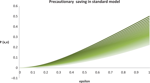
Precautionary Saving in standard model (ωλ=1) : Darker (higher from below) lines represent the savings when the cash on hand (x) is lower.

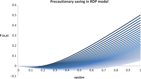
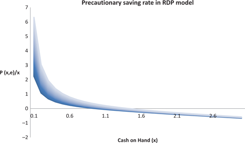
5.2 RDP Precautionary Saving

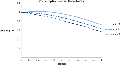
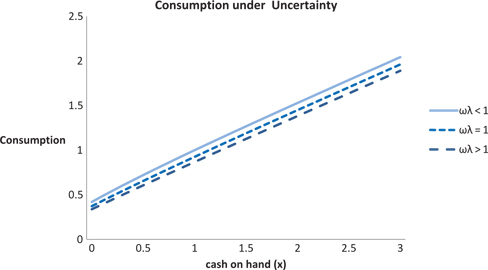
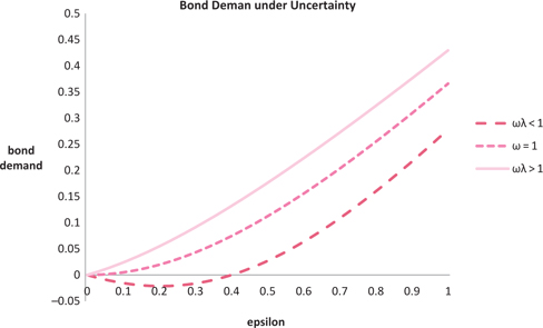
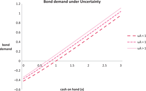
In the reference-dependence model, the consumption and saving profiles are affected by the gain-loss parameters. The loss aversion arises here with respect to bad outcomes due to uncertainty. Thus, as explained by eq. [15], high loss aversion (ωλ>1) implies that people save more than in the standard uncertainty model (ωλ=1). Likewise, low loss aversion (ωλ<1) implies that people save less than in the standard model. The closed form state-independent RDP consumption and saving functions are

[28]c0RDP=3(1+x)4+εη(ωλ−1)2−12K(x,ε,ηλω)

[29]b1RDP=x−34−εη(ωλ−1)2+12K(x,ε,ηλω)

[30]c1RDP=1+x4∓εη(ωλ−1)2+12K(x,ε,ηλω)

[31]K(x,ε,ηωλ)={3(1+x)/2+εη(ωλ−1)}2−2[1+2x+x2−ε2]

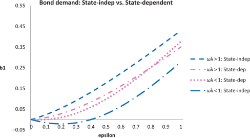
The following (Figures 2, 3, 4, 5) show c0 and b1 as functions of x or ε for different values of ε or x. Each figure demonstrates either the consumption or the saving behavior of the reference-dependent consumers with three different specifications of the loss aversion parameter (ωλ=><1). When ωλ=1, this represents the standard model. Figure 3 displays the first-period consumption for the three different models. In the figure, all the models predict higher consumption as the DMs have more cash on hand. But given the cash on hand, the DM with the least loss aversion would consume more in the first period by saving less for the future. Figure 5 suggests the same reasoning with respect to saving because saving is defined by b1=y0−c0, and current consumption and saving move in opposite directions. Figures 2 and 4 jointly show that if the uncertainty level is not severe, the DM with low loss aversion (ωλ<1) may want to overconsume (c0>1) even by borrowing or dissaving (b1<0). Unlike those who have high loss aversion, these consumers have a relatively low feeling of loss when a low outcome is realized. Because the loss is not more painful than the gain is pleasant, their overall utilities are not lowered much even when the bad outcome happens. Thus, they have little incentive to save to compensate for their feeling of loss in a bad situation and are sometimes tempted to consume more by borrowing. The precautionary saving is

[32]PRDP(x;ε)=−(1+x)4−εη(ωλ−1)2+12K(x,ε,η,ωλ)

The next two figures (Figures 6 and 7) show PRDP(x;ε) and PRDP/x (for x>0) as functions of x or ε.Figure 6 describes that given ε, the precautionary saving motive will be lowered if the consumer has a high level of cash on hand. However, given a level of cash on hand, higher income uncertainty increases the precautionary saving motive. But with DM who has a low loss aversion parameter, the precautionary saving can be negative (borrowing) under minor income shocks. When either ωλ=1 or η=0, the RDP precautionary saving function collapses to the standard saving function under uncertainty above. Now let us set x=1 to get the consumption and saving profile of the DM with RDP at partial equilibrium:

[33]c0RDP=32+εη(ωλ−1)2−121+2ε2+6εη(ωλ−1)+ε2η2(ωλ−1)2

[34]b1RDP=−12−εη(ωλ−1)2+121+2ε2+6εη(ωλ−1)+ε2η2(ωλ−1)2

[35]c1RDP=12∓εη(ωλ−1)2+121+2ε2+6εη(ωλ−1)+ε2η2(ωλ−1)2

Figure 2:

RDP plots of c0 when x=1. The loss aversion parameters are ωλ=0.8,ωλ=1, and ωλ=1.2.

Figure 3:

RDP plots of c0 when ε=0.4. The loss aversion parameters are ωλ=0.8,ωλ=1, and ωλ=1.2.

Figure 4:

RDP plots of b1 when x=1. The loss aversion parameters are ωλ=0.8,ωλ=1, and ωλ=1.2. When ωλ<1, the bond demand can be negative.

Figure 5:

RDP plots of b1 when ε=0.4. The loss aversion parameters are ωλ=0.8,ωλ=1, and ωλ=1.2. Each bond demand cuts b1=0 at x≤1.

Figure 6:

RDP(ωλ=0.8) Precautionary Saving: the darker (higher from below) lines are from lower cash on hand (x).

Figure 7:

RDP(ωλ=0.8) Precautionary saving rate: the darker (closer to the origin) lines are from lower epsilon (ε).

First, let us examine the bond demand. If ωλ=1, i.e. the standard model, the bond demand is b1=12[1+2ε2−1]>0 and the value of this function increases as ε increases. How about the case when ωλ>1? When ωλ>1, it is true that a high ε decreases the second term, but increases the third term. Because 6εη(ωλ−1)>0, the bond demand increases unambiguously more in the reference-dependence model than in the standard model. This implies that given a value of uncertainty parameter ε, the DM, with loss aversion to bad situation, saves more than the DM without this feeling. If, however, ωλ<1, the overall effect is ambiguous depending on the magnitude of ε and ωλ. Second, let us look at the first period consumption c0RDP with respect to ε. If ωλ=1, then a high ε decreases current consumption. If ωλ>1, then a high ε increases the second term but decreases the third term. By the same argument as in the bond demand case, current consumption decreases unambiguously more in the reference-dependent utility model than in the standard model. If ωλ<1, then for a given value of η, a high ε induces lower current consumption c0 when ε>6/(1−ωλ) but higher current consumption c0 when ε<6/(1−ωλ). ^[31] This suggests that for the case of typical income uncertainty without huge fluctuation, the effect is positive when ωλ<1. Under modest income uncertainty, the RDP effect on consumption is positive for this case. That is, those who care less about the pain from future loss may deviate from typical saving for more present consumption.

5.3 RDP-Dep Precautionary Saving

In the example of the two-period consumption-saving model, in which the consumption and reference points are positively related, the state-dependent RDP maximization problem is given by

[36]Maxlnc0+β12lnc1h+12lnc1l

+βη12lnc1h−lnc1l+ωλ12lnc1l−lnc1h

subjectto

c0+b1=y0

c1=y˜1+Rb1

Unlike the state-independent case, the gain or loss utility arises with p=1/2 instead of p=1/4. The optimality condition leads to

[37]c0−1=Rβ12c1h−1+12c1l−1+η(ωλ−1)12c1l−1−c1h−1.

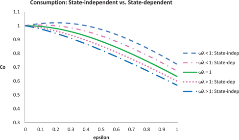
Excepting the third term, this optimality condition is equal to that of the state-independent RDP in previous subsection. Compared to state-independent RDP, for those who have a high loss aversion (ωλ>1), the DM's intention to save more due to loss aversion is slightly weaker with state-dependent RDP. The state-dependent consumption-saving profile is

[38]c0RDP(dep)=3x2+εη(ωλ−1)4−12K(x,ε,ηωλ)

[39]b1RDP(dep)=−x2−εη(ωλ−1)4+12K(x,ε,ηωλ)

[40]c1RDP(dep)=2−x2∓εη(ωλ−1)4+12K(x,ε,ηωλ)

[41]K(x,ε,ηωλ)=x2+3xεη(ωλ−1)+{εη(ωλ−1)/2}2+2ε2.

Likewise, the precautionary saving is obtained from

[42]PRDP(dep)(x;ε)=−x2−εη(ωλ−1)2+12K(x,ε,ηωλ).

However, it is still true that if ωλ=1 or η=0, this indicates the case of the standard model. The consumption and saving at x=1 are

[43]c0RDP=32+εη(ωλ−1)4−12K(x,ε,ηωλ)

[44]b1RDP=−12−εη(ωλ−1)4+12K(x,ε,ηωλ)

[45]c1RDP=12∓εη(ωλ−1)4+12K(x,ε,ηωλ)

[46]K(x,ε,ηωλ)=1+3εη(ωλ−1)+{εη(ωλ−1)/2}2+2ε2.

Figure 8 displays RDP consumption when x=1 for both state-independent and state-dependent reference specifications. As seen in the figure, a state-independent model implies lower consumption in the first period due to stronger precautionary saving motivation. ^[32]Figure 9 displays RDP bond demands when x=1 for both state-independent and state-dependent models. From the figure, it is clear that state-dependent RDP model generates less savings or smaller over-consumption intensity than in the state-independent RDP world.

Figure 8:

RDP plots of c0 when x=1 for both state-independent and state-dependent specifications. The loss aversion parameters are ωλ=0.8,ωλ=1, and ωλ=1.2.

Figure 9:

RDP plots of b1 when x=1 for both state-independent and state-dependent specifications. The loss aversion parameters are ωλ=0.8 and ωλ=1.2.

6 General Equilibrium

In this section, we analyze equilibrium savings related to interest rates in a general equilibrium model, in which the economy is populated by two types of agents who are different in their degrees of loss aversion, but identical otherwise. Though it is possible to construct a general equilibrium model between loss-averse agents and standard agents {ωAλ>1 and ωBλ=1}, it is more useful to assume that {ωAλ>1 and ωBλ<1} because in an economy with two types of identical agents, one type of agents must save (lend) while the other must borrow to clear the market. The first specification may not generate this structure. Unlike in the partial equilibrium case, the bond price or the interest rate is not fixed in general equilibrium, and it is determined in the market by the term that the net supply of bonds equals zero: bond prices clear the market at equilibrium.

6.1 State-Independent RDP

From eq. [15], we know that each type of DM meets one of the following optimality condition:

[47]c0−1=Rβ12c1h−1+12c1l−1+η(ωAλ−1)1212c1l−1−c1h−1

[48]c0−1=Rβ12c1h−1+12c1l−1−η(1−ωBλ)1212(c1l−1−c1h−1)

How can we compare the two? Because ωAλ>1 and ωBλ<1 it is expected that

[49]−η(1−ωBλ)1212(c1l−1−c1h−1)<η(ωAλ−1)1212(c1l−1−c1h−1)

This implies that the three gain-loss marginal utilities satisfy: MUG−L(c1ωλ<1)<MUG−L(c1ωλ=1)<MUG−L(c1ωλ>1). Thus, the DM with ωBλ<1 would not save more than the DM with ωAλ>1 would save. To derive a general equilibrium result for the different types of agents, we need a price to clear the saving/borrowing market. Therefore, it is necessary to determine the bond demand as a function of interest rates. For simplicity we keep assuming β=1/R. Under the assumption of y0=1, together with y1h=1+ε and y1l=1−ε, the first order condition implies

[50]4[1+R+ε−Rc0)][1+R−ε−Rc0]c0

=[1+ε+R−Rc0][2−4(1−ωλ)]+[1−ε+R−Rc0][2+4(1−ωλ)]

Solving the equation brings consumption c0 as a function of the interest rate and thus bond demand is obtained by b1(R)=y0−c0(R). The bond demand of the DM(A) who is loss averse (ωAλ>1) is

(51)b1A=−(1+R)−2εη(ωAλ−1)2R(R+1)

+[(2R+1)(1+R)+2εη(ωAλ−1)]2−4(R+1)R[(1+R)2−ε2]2R(R+1)

while the bond demand of the DM(B) who is tolerant to loss (ωBλ<1) is

[52]b1B=−(1+R)+2εη(1−ωBλ)2R(R+1)

+[(2R+1)(1+R)−2εη(1−ωBλ)]2−4(R+1)R[(1+R)2−ε2]2R(R+1)

Now let us introduce a market clearing condition for the economy. Assume that there are only two types of agents in the economy and that their intensity of loss aversion/tolerance is symmetric, i.e. ωAλ−1=1−ωBλ. Assume further that the portion of those who are loss averse (type A) is θ. Initially let us set θ=1/2.Figure 10 shows the bond demand by the two different DMs. The uncertainty specification is ε=0.2. With an equal distribution of the two types of agents, the bond market yields positive net savings as seen in the figure and therefore the market is not in equilibrium. Under the assumption of θ=1/2, together with the symmetric intensity level of loss aversion in the simple model, it is found that positive net savings are persistent ^[33] even with a very low uncertainty level. ^[34]Figure 11 summarizes the result when the economy is equally populated by both types of agents.

Figure 10:

The state-independent bond demand with θ=1/2: the two agents are represented by λωA=1.2 and λωB=0.8. The uncertainty is given by ε=0.2.

Figure 11:

The state-independent net saving of the economy with θ=1/2: the two agents are represented by λωA=1.2 and λωB=0.8.

This implies that the economy should have more of the savers to lower the interest rate to meet the borrowers. In fact, a higher θ about 2/3, namely,θ=0.659646 induces zero net savings for the uncertainty level: to clear the bond market, it should be satisfied that

[53]θb1A+(1−θ)b1B=0

where 0<θ<1. Figure 12 shows the general equilibrium result for two different DMs with asymmetric intensity parameters, ωAλ=2 and ωBλ=0.2. The uncertainty specification is ε=0.2, and θ is adjusted accordingly to set an equilibrium for each level of the gross interest rates.

Figure 12:

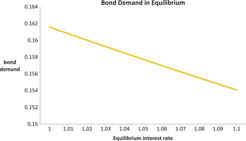
The state-independent equilibrium bond demand: the two agents are represented by λωA=2 and λωB=0.2. The uncertainty is given by ε=0.2.

6.2 State-dependent RDP and Comparison

Following the similar steps as those in the state-independent RDP, the optimality condition for the two types of agents in the state-dependent model is given by:

The bond demand of the DM(A) who is loss averse (ωAλ>1) is

while the bond demand of the DM(B) who is tolerant of loss (ωBλ<1) is

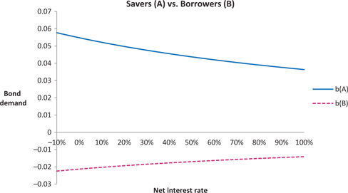
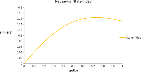
Figure 13 explains the saving and borrowing behaviors when the economy has an equal population of the two types of agents with both state-independent and state-dependent reference dependences. From the figure, it is clear that both borrowing and saving amounts are smaller for all levels of interest rates with the state-dependent model. Figure 14 demonstrates the variation in net savings corresponding to the uncertainty level. From this we may infer that for all levels of income uncertainty, 0<ε<1, we may achieve equilibrium easily in a state-dependent world. Moreover, in a state-dependent world, a minor adjustment of θ from 1/2 would cause an equilibrium point to be achieved, which in fact is not expected in the state-independent world.

Figure 13:

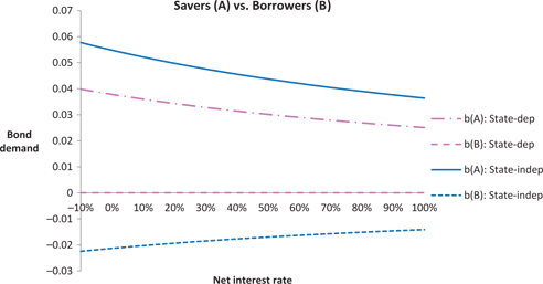
The state-independent and state-dependent bond demands with θ=1/2: the two agents are represented by λωA=1.2 and λωB=0.8. The uncertainty is given by ε=0.2.

Figure 14:

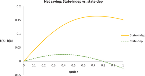
The state-independent and state-dependent net savings of the economy with θ=1/2: the two agents are represented by λωA=1.2 and λωB=0.8.

7 Conclusion

In this paper, we study a model of reference-dependent preferences with endogenous reference expectations under the two schemes of state-independent and state-dependent stochastic references points. A key issue in reference-dependent utility models is the reference point, because as Pesendorfer (2006) claims, a reference point can be anything and may be selected arbitrarily by researchers. Often the reference point is assumed to be a current status, such as current consumption, position, or endowment. In this paper, we build a tractable, intertemporal choice model following two recent developments regarding expectation-based reference points: state-independent reference expectations, which originated in disappointment theory, and state-dependent reference expectations, which are based on regret theory.

We build the model according to the novel notion that some individuals might be loss-tolerant. Because of this assumption, we can provide a richer analysis that helps us better understand the consumption and precautionary saving behaviors of different types of consumers. Moreover, the model we develop has many merits in terms of economic modeling, in that it departs from typical aspects of reference-dependence, such as habit formation; adapts forward looking expectations; and uses realistic preference specifications.

In the two-period consumption-saving model, we derive analytic solutions to show that, when loss aversion is high, the decision maker saves more than the standard model predicts and thus consumes less in the current period. However, when the loss aversion is low, the overall result is ambiguous, although the decision maker may even want to borrow to consume more for the current period if he faces mild uncertainty relative to the intensity of his loss aversion. Given the same intensity of loss aversion, we find that the state-dependent model generates a smaller deviation than the standard one for both consumption and precautionary saving. Consequently, it is implied that for positively related consumption and its reference points, the state-independent model tends to exaggerate the true outcome of gain-loss feeling and vice versa. In both of the models, the meaning of precautionary saving can be defined in a different way from the standard model under uncertainty, although the size of this effect depends on whether it is state-dependent or not. Throughout this paper, we show that precautionary saving behavior is closely related to the degree of loss aversion, by which the decision makers may deviate for more or less consumption (and thus less or more saving) than what the standard uncertainty model predicts. Finally, from the general equilibrium exercise, we find that at a given uncertainty level, both borrowings and savings are smaller for all levels of interest rates with the state-dependent model. Also for all levels of income uncertainty, the state-dependent model agrees more with the even distribution of borrowers and savers.

References

Aizenman, J. 1998. “Buffer Stocks and Precautionary Savings with Loss Aversion.” Journal of International Money and Finance 17:931–47.10.1016/S0261-5606(98)00035-7Search in Google Scholar
Andersen, S., G. Harrison, M. Lau, and E. Rutström. 2008. “Eliciting Risk and Time Preferences.” Econometrica 76:583–618.10.1111/j.1468-0262.2008.00848.xSearch in Google Scholar
Bowman, D., D. Minehart, and M. Rabin. 1999. “Loss Aversion in a Consumption-Savings Model.” Journal of Economic Behavior and Organization 38:155–78.10.1016/S0167-2681(99)00004-9Search in Google Scholar
Carroll, C. D. 1997. “Buffer-Stock Saving and the Life-Cycle/Permanent Income Hypothesis.” Quarterly Journal of Economics 112:1–55.10.3386/w5788Search in Google Scholar
Chetty, R., and A. Szeidl. 2010. “Consumption Commitments: A Foundation for Reference-Dependent Preferences and Habit Formation.” Working Paper.Search in Google Scholar
Cillo, A., and P. Delquie. 2006. “Disappointment Without Prior Expectations: A Unifying Perspective on Decision Under Risk.” Journal of Risk and Uncertainty 33:197–215.10.1007/s11166-006-0499-4Search in Google Scholar
Deaton, A. 1991. “Saving and Liquidity Constraints.” Econometrica 59:1221–48.10.3386/w3196Search in Google Scholar
Feigenbaum, J. 2008. “Information Shocks and Precautionary Saving.” Journal of Economic Dynamics and Control 32:3917–38.10.1016/j.jedc.2008.04.008Search in Google Scholar
Feigenbaum, J. 2009. “Precautionary Saving Unfettered.” Working Paper, University of Pittsburgh.Search in Google Scholar
Freeman, D. 2013. “Revealed Preference Foundations of Expectations-Based Reference-Dependence.” Working paper.Search in Google Scholar
Giorgi, E., and T. Posty. 2011. “Loss Aversion with a State-Dependent Reference Point.” Management Science 57:1094–110.10.1287/mnsc.1110.1338Search in Google Scholar
Gourinchas, P., and J. A. Parker. 2002. “Consumption Over the Life Cycle.” Econometrica 70:47–89.10.3386/w7271Search in Google Scholar
Gul, F. 1991. “A Theory of Disappointment Aversion.” Econometrica 59:667–86.10.2307/2938223Search in Google Scholar
Halevy, Y., and V. Felkamp. 2005. “A Baysian Approach to Uncertainty Aversion.” Review of Economic Studies 72:449–66.10.1111/j.1467-937X.2005.00339.xSearch in Google Scholar
Kahneman, D., and A. Tversky. 1979. “Prospect Theory: An Analysis of Decision Under Risk.” Econometrica 47:263–91.10.21236/ADA045771Search in Google Scholar
Kobberling, V., and P. Wakker. 2005. “An Index of Loss Aversion.” Journal of Economic Theory 122:119–31.10.1016/j.jet.2004.03.009Search in Google Scholar
Krähmer, D., and R. Stone. 2013. “Anticipated Regret as an Explanation of Uncertainty Aversion.” Economic Theory 52:709–28.10.1007/s00199-011-0661-3Search in Google Scholar
Köszegi, B., and M. Rabin. 2006. “A Model of Reference-Dependent Preferences.” Quarterly Journal of Economics 121:1133–165.Search in Google Scholar
Köszegi, B., and M. Rabin. 2007. “Reference-Dependent Risk Attitudes.” American Economic Review 97:1047–73.10.1257/aer.97.4.1047Search in Google Scholar
Köszegi, B., and M. Rabin. 2009. “Reference-Dependent Consumption Plans.” American Economic Review 99:909–36.10.1257/aer.99.3.909Search in Google Scholar
Ludvigson, S. C., and A. Michaelides. 2001. “Does Buffer-Stock Saving Explain the Smoothness and Excess Sensitivity of Consumption?” American Economic Review 91:631–47.10.1257/aer.91.3.631Search in Google Scholar
Pagel, M. 2013. “Expectations-Based Reference-Dependent Life-Cycle Consumption.” Working Paper.10.2139/ssrn.2268254Search in Google Scholar
Park, H. 2015. “Bounded Rationality and Lifecycle Consumption.” Working paper.Search in Google Scholar
Pasquariello, P. 2014. “Prospect Theory and Market Quality.” Journal of Economic Theory 149:276–310.10.1016/j.jet.2013.09.010Search in Google Scholar
Pesendorfer, W. 2006. “Behavioral Economics Comes of Age: A Review Essay on ‘Advances in Behavioral Economics’”. Journal of Economic Literature 44:712–21.10.1257/jel.44.3.712Search in Google Scholar
Rabin, M. 2000. “Risk Aversion and Expected-Utility Theory: A Calibration Theorem.” Econometrica 68:1281–92.10.1142/9789814417358_0013Search in Google Scholar
Siegmann, A. 2002. “Optimal Saving Rules for Loss-Averse Agents Under Uncertainty.” Economics Letters 77:27–34.10.1016/S0165-1765(02)00113-1Search in Google Scholar
Sugden, R. 2003. “Reference-Dependent Subjective Expected Utility.” Journal of Economic Theory 111:172–91.10.1016/S0022-0531(03)00082-6Search in Google Scholar
Tversky, A., and D. Kahneman. 1992. “Advances in prospect theory: Cumulative representation of uncertainty.” Journal of Risk and Uncertainty 5:297–323.10.1007/BF00122574Search in Google Scholar
©2016 by De Gruyter
Articles in the same Issue
- Frontmatter
- Research Articles
- Currency Exchange in an Open-Economy Random Search Model
- Relative Concerns on Visible Consumption: A Source of Economic Distortions
- Workplace Deviance and Recession
- Strategic Delay in Global Games
- Assortative Outsourcing with Exit
- On the Impossibility of Fair Risk Allocation
- Price and Inventory Dynamics in an Oligopoly Industry: A Framework for Commodity Markets
- The Dynamics of Incentives, Productivity, and Operational Risk
- Dynamic Contests With Bankruptcy: The Despair Effect
- Welfare-Improving Effect of a Small Number of Followers in a Stackelberg Model
- The Predominant Role of Signal Precision in Experimental Beauty Contests