The Predominant Role of Signal Precision in Experimental Beauty Contests

Romain Baeriswyl; Camille Cornand

doi:10.1515/bejte-2015-0002

Artikel Öffentlich zugänglich

The Predominant Role of Signal Precision in Experimental Beauty Contests

Romain Baeriswyl und Camille Cornand

Veröffentlicht/Copyright: 3. Dezember 2015

Veröffentlicht von

Veröffentlichen auch Sie bei De Gruyter Brill

Manuskript einreichen Informationen für Autor*innen Erkunden Sie dieses Fachgebiet

Aus der Zeitschrift The B.E. Journal of Theoretical Economics Band 16 Heft 1

Abstract

The weight assigned to public information in Keynesian beauty contests depends on both the precision of signals and the degree of strategic complementarities. This experimental study shows that the response of subjects to changes in signal precision and the degree of strategic complementarities is qualitatively consistent with theoretical predictions, though quantitatively weaker. The weaker response of subjects to changes in the precision of signals, however, mainly drives the weight observed in the experiment, qualifying the role of strategic complementarities and overreaction in experimental beauty contests.

Keywords: heterogeneous information; beauty contest; experiment; public information

JEL classification: C92; D82; D84; E58

1 Introduction

In coordination games under heterogeneous information, public information plays a double role. While public information conveys information about economic fundamentals, it also conveys strategic information because it constitutes common knowledge among all market participants. Fundamental uncertainty is driven by the precision of signals, strategic uncertainty by the degree of strategic complementarities. The weight assigned to public information in equilibrium, thus, depends on both the precision of signals and the degree of strategic complementarities. As shown by Morris and Shin (2002), the coordination motive leads agents to overreact to public information in the sense that the equilibrium weight assigned to it is larger than can be justified by its information about fundamentals.

Several studies have identified the occurrence of overreaction in laboratory experiments. ^[1] For instance, the experimental analysis by Cornand and Heinemann (2014) measures subjects’ overreaction to public information when varying the degree of strategic complementarities. However, while the role of the precision of the public signal is as essential as strategic complementarities for the determination of equilibrium weight, it has hardly been studied. This paper fills this gap.

We run an experiment built on the beauty contest game of Morris and Shin (2002). In this game, agents have to choose actions that are as close as possible both to a fundamental and to the actions of others. To decide on their actions, agents receive both a public signal and a private signal about the fundamental. The equilibrium weight assigned to public information increases with both its precision and the degree of strategic complementarities. We test predictions of this beauty contest game when varying the precision of public information and the degree of strategic complementarities.

In line with theory, the weight assigned to public information increases with its precision both in the first-order expectation of the fundamental and in the beauty contest action. However, the effect of precision is weaker than theoretically predicted: subjects underweight precise public signals and overweight imprecise public signals both in the first-order expectation of the fundamental and in the beauty contest action.

The experiment also exhibits overreaction in the sense of Morris and Shin (2002), but only when the weight assigned to the public signal in the beauty contest is compared to the weight in the first-order expectation observed in the experiment. The overreaction in the beauty contest is nevertheless weaker than theoretically predicted and can be explained with limited levels of reasoning, which is consistent with Nagel (1995) or Cornand and Heinemann (2014).

By contrast, comparing the weight in the experimental beauty contest with the theoretical weight in the first-order expectation does not systematically show overreaction, because the underweighting of precise public information in the first-order expectation may dominate the overreaction due to strategic complementarities, such that the weight observed in the beauty contest is lower than the theoretical weight in the first-order expectation. Respectively, because subjects overweight imprecise public information, the weight assigned to it both in the first-order expectation and in the beauty contest action is higher than the theoretical weight in the beauty contest action. This suggests that the issue of overweighting/underweighting imprecise/precise information matters more than overreaction to public information. Fundamental uncertainty may dominate strategic uncertainty in the beauty contest.

This paper contributes to a growing experimental literature related to the effects of public vs. private information in games with strategic complementarities. ^[2]Cornand (2006) and Cornand and Heinemann (2014) render account for overreaction to public signals. Baeriswyl and Cornand (2014) test the effectiveness of two communication strategies – partial publicity consisting of the disclosure of transparent information as a semi-public signal to a fraction of market participants only and partial transparency consisting of the disclosure of ambiguous public information to all market participants – to reduce market overreaction. Shapiro, Shi, and Zillante (2014) show that the predictive power of the level-k reasoning approach is related to the strength of the coordination motive and the symmetry of information. None of these papers focuses on the role of information precision. To our knowledge, in the beauty contest game proposed by Morris and Shin (2002), Dale and Morgan (2012) are the first to analyze what impact the precision of the signals has. They show that subjects place an inefficiently high weight on a public signal of low accuracy, which is in line with our results. However, they do not elicit beliefs on the fundamental, so that they cannot disentangle the specific effect of precision on the first-order expectation and the beauty contest. ^[3]

The rest of the paper is structured as follows. Section 2 presents the theoretical framework and Section 3 the experiment. Results are stated in Section 4. Section 5 discusses the results in terms of policy implications and concludes.

2 The Theoretical Model

The spirit of the Keynesian beauty contest is characterized by strategic complementarities in agents’ decision rules: each agent takes its decision not only according to its expectation of economic fundamentals but also according to its expectation of other agents’ decisions. The utility function for agent i is given by:

ui(ai,θ)≡−(1−r)(ai−θ)2−r(ai−a−i)2,

where θ is the fundamental, ai is the action taken by agent i, a−i is the average action taken by other agents −i, and r is a constant. Maximizing utility yields the optimal action of agent i:

ai=(1−r)Ei(θ)+rEi(a−i).

The parameter r is the weight assigned to the strategic component which drives the strength of the coordination motive in the decision rule. Assuming 0≤r<1 implies that decisions are strategic complements: agents tend to align their decisions with those of others. ^[4] Following the insight of Morris and Shin (2002) (henceforth MS), the optimal action in the Keynesian beauty contest is derived under imperfect, heterogenous information.

2.1 Information Structure

Each agent i receives a private signal xi and a public signal y. These signals deviate from the fundamental θ by some error terms with uniform distribution. Whereas the private signal xi=θ+εi with εi∼U[−με+με] is different for each agent i, the public signal y=θ+η with η∼U[−μη+μη] is the same for all agents and is common knowledge among them. Noise terms εi of distinct agents and the noise η of the public signal are independent and their distribution is treated as exogenously given.

2.2 Equilibrium

To derive the perfect Bayesian equilibrium action of agents, we substitute successively the expected average action of other participants with higher-order expectations about the fundamental:

ai=Ei(1−r)θ+ra−i

=Ei[(1−r)θ+r[E¯−i[(1−r)θ+r[E¯−i[(1−r)θ+…]]]]]

[1]=(1−r)∑k=0∞rkEi[E¯−ik(θ)],

where k is the degree of higher-order iteration, and E¯−i(.)=∫−iEi(.)d(−i) is the average expectation operator of other agents. We use the following notation of higher-order expectations: E¯−i0(x)=x, E¯−i1(x)=E¯−i(x), E¯−i2(x)=E¯−iE¯−i(x), and so on.

With error terms uniformly distributed, the first-order expectation of agent i with regard to the fundamental θ conditional on his private and public information corresponds to the middle of the intersection of the intervals [xi−με,xi+με] and [y−μη,y+μη], and yields

E(θ|xi,y)=max{xi−με;y−μη}+min{xi+με;y+μη}2

[2]=(1−fi)⋅xi+fi⋅y.

The weight assigned to the public signal y in the first-order expectation, fi, is dependent on the signal draw.

As derived in Appendix A, the average first-order expectation of other agents with regard to the fundamental θ is written as

E¯−i(θ)=(1−f)⋅x¯−i+f⋅y,

where f represents the average weight assigned to y by other agents, where each agent estimates θ according to (2), and x¯−i=∫−ix−i d(−i).

Using Ei(xˉ−i)=Ei(θ), the second and higher-order expectations yield

EiE¯−i(θ)=(1−f)(1−fi)⋅xi+(1−(1−f)(1−fi))⋅y,

EiE¯−ik(θ)=(1−f)k(1−fi)⋅xi+(1−(1−f)k(1−fi))⋅y,

and plugging higher-order expectations of the fundamental into (1), the individual action becomes

ai=(1−r)∑k=0∞rkE[E¯−ik(θ)]

=(1−r)∑k=0∞rk(1−f)k(1−fi)⋅xi+1−(1−f)k(1−fi)⋅y

=(1−r)(1−fi)1−r(1−f)⏟1−wixi+(1−r)fi+rf1−r(1−f)⏟wiy.

The expected average action is

E(a−i)=(1−r)(1−f)1−r(1−f)⏟1−wθ+f1−r(1−f)⏟wy.

The overreaction in the sense of MS is characterized by the fact that the weight assigned to the public signal y in the optimal action is larger than in the first-order expectation: w=f/(1−r(1−f))>f.

3 The Experiment

To analyze the role of the precision of signals in the coordination game, we run an experiment with three treatments, each corresponding to a different degree of relative precision of the private and public signals.

3.1 Experimental Procedure

We conducted 6 sessions with a total of 108 participants. Sessions were run at the GATE lab in Lyon, France. Participants were mainly students from Lyon University, the engineering school, Ecole Centrale Lyon, and EM Lyon business school. In each session, the 18 participants were separated into three independent groups of 6 participants each. Each participant could only take part in one session. Each session consisted of three stages, composed of 10 periods each (thus a total of 30 periods per session). Each stage corresponded to a different treatment. Participants played within the same group throughout the whole length of the experiment and did not know the identity of the other participants in their group. Subjects were seated at PCs in a random order. Instructions were then read aloud and questions answered in private. Throughout the sessions, participants were not allowed to communicate with one another and could not see each others’ screens. Before starting the experiment, participants were required to answer a few questions to ascertain their understanding of the rules. The experiment started after all participants had given the correct answers to these questions. Examples of instructions, questionnaire and screens are given in Appendices B, C, and D.

The program was written using z-Tree experimental software (Fischbacher (2007)) and participants were recruited via ORSEE.

3.2 Treatment Parameters and Theoretical Predictions

In every period and for each group, a fundamental state θ is drawn randomly using a uniform distribution from the interval [50,950]. ^[5] In every period of the experiment, each subject has to make two decisions:

Each subject forms his best expectation ei about the fundamental θ (decision 1). The payoff function in ECU (experimental currency units) for subject i related to his estimation is given by

u(ei,θ)=200−(ei−θ)2.

Each subject decides on an action ai in the beauty contest (decision 2). The payoff function in ECU for subject i is given by

u(ai,a−i,θ)=400−1.5(ai−θ)2−8.5(ai−a−i)2,

in sessions 1 to 4 and by

u(ai,a−i,θ)=350−(ai−θ)2−(ai−a−i)2,

in sessions 5 and 6, where a−i is the average action of other subjects of the same group.

To make their decisions, subjects receive two signals on the fundamental θ and are forced to choose a weighted average of the signals they get as their decisions. ^[6]

After each period, subjects were informed about the true state, their partner’s decision and their payoff. Information about past periods from the same stage (including signals and their own decisions) was displayed during the decision phase on the lower part of the screen. At the end of each session, the ECU earned were summed up and converted into euros. 1000 ECU were converted to 2 euros. ^[7]

The choice of parameters for the experiment is summarized in Table 1. Column tf shows the average optimal weight assigned to the public signal in decision 1 (the first-order expectation of the fundamental θ, as derived in Appendix A) and column tw shows the average optimal equilibrium weight in decision 2 (the beauty contest).

Table 1:

Experiment parameters, average optimal weight on y in decisions 1 (tf) and 2 (tw).

Sessions	Groups	Players	Stage	Periods	r	με	μη	tf	tw
1–2	1–6	6	1	10	0.85	10	10	0.50	0.87
			2	10	0.85	10	5	0.91	0.98
			3	10	0.85	10	20	0.09	0.39
3–4	7–12	6	1	10	0.85	10	10	0.50	0.87
			2	10	0.85	10	20	0.09	0.39
			3	10	0.85	10	5	0.91	0.98
5–6	13–18	6	1	10	0.5	10	10	0.50	0.67
			2	10	0.5	10	5	0.91	0.95
			3	10	0.5	10	20	0.09	0.16

Each subject receives both a public and a private signal as described in Section 2.1. The private signal received by each subject is distributed as xi∼U[θ−10,θ+10]. The distribution of the public signal differs, depending on the treatment. As reported in Table 1, the order of play is different in sessions 1, 2, 5, and 6 from that in sessions 3 and 4. In sessions 1, 2, 5, and 6, the public signal is drawn from y∼U[θ−5,θ+5] in stage 2 and from y∼U[θ−20,θ+20] in stage 3. In sessions 3 and 4, the public signal is drawn from y∈[θ−20,θ+20] in stage 2 and from y∼U[θ−5,θ+5] in stage 3.

4 The Results

The observed average weight assigned in the experiment to the public signal in decision 1 (of) is reported in Table 2, while the observed average weight assigned to the public signal in decision 2 (ow) is reported in Table 3. ^[8]tfcond and twcond denote the theoretical weight conditional on the realization of signals in the experiment. Respectively, tfuncond and twuncond denote the theoretical weight unconditional on the realization of signals. Figure 1 compares the observed average weight assigned to the public signal in decisions 1 (of) and 2 (ow) to their theoretical unconditional value for each treatment over 10 periods. ^[9]

Figure 1:

Average weight assigned to the public signal in decision 1 f (first-order expectation) and in decision 2 w (beauty contest).

First, we analyze the weight on the public signal in the stated first-order expectation. We then compare weights in the first-order expectation to that in the beauty contest to measure overreaction, and discuss the effect of information precision and of the degree of strategic complementarities on the beauty contest. Statistical tests are based on Wilcoxon rank sum tests when comparing observed data to theoretical predictions and on Wilcoxon matched-pairs signed-rank tests for between treatment tests. The fact that we cannot detect order effects ^[10] allows us to pool together data from groups 1 to 12 for the remaining analysis.

Table 2:

Average weight on y in the expectation of the fundamental (decision 1).

Sessions	Groups	μη=10		μη=5		μη=20
		of	tfcond	of	tfcond	of	tfcond
1	1	0.54	0.50	0.77	0.90	0.33	0.12
1	2	0.46	0.50	0.65	0.89	0.31	0.09
1	3	0.48	0.50	0.76	0.89	0.30	0.11
2	4	0.48	0.50	0.70	0.90	0.41	0.07
2	5	0.53	0.50	0.73	0.89	0.44	0.07
2	6	0.53	0.50	0.71	0.87	0.30	0.07
3	7	0.52	0.50	0.64	0.89	0.43	0.09
3	8	0.51	0.50	0.81	0.90	0.35	0.18
3	9	0.51	0.50	0.71	0.90	0.36	0.08
4	10	0.45	0.50	0.83	0.90	0.32	0.12
4	11	0.51	0.50	0.79	0.90	0.36	0.08
4	12	0.51	0.50	0.81	0.89	0.37	0.14
5	13	0.52	0.50	0.77	0.91	0.34	0.11
5	14	0.54	0.50	0.72	0.90	0.37	0.08
5	15	0.56	0.50	0.59	0.91	0.39	0.12
6	16	0.49	0.50	0.78	0.89	0.41	0.11
6	17	0.48	0.50	0.61	0.91	0.32	0.08
6	18	0.50	0.50	0.62	0.88	0.40	0.10
Average	1–18	0.51	0.50	0.72	0.90	0.36	0.10
tfuncond	13–18	0.50		0.91		0.09

Table 3:

Average weight on y in the beauty contest (decision 2).

Sessions	Groups	μη=10		μη=5		μη=20
		ow	tw_cond	ow	tw_cond	ow	tw_cond
1	1	0.73	0.87	0.82	0.98	0.53	0.42
1	2	0.70	0.87	0.83	0.98	0.61	0.40
1	3	0.88	0.87	0.96	0.98	0.67	0.41
2	4	0.63	0.87	0.81	0.98	0.58	0.38
2	5	0.81	0.87	0.96	0.98	0.80	0.38
2	6	0.80	0.87	0.87	0.98	0.78	0.38
3	7	0.70	0.87	0.73	0.98	0.61	0.40
3	8	0.82	0.87	0.86	0.98	0.58	0.46
3	9	0.76	0.87	0.84	0.98	0.70	0.39
4	10	0.74	0.87	0.91	0.98	0.48	0.42
4	11	0.78	0.87	0.86	0.98	0.51	0.39
4	12	0.65	0.87	0.83	0.98	0.45	0.43
Average	1–12	0.75	0.87	0.86	0.98	0.61	0.41
twuncond	1–12	0.87		0.99		0.39
5	13	0.67	0.67	0.79	0.95	0.44	0.18
5	14	0.72	0.67	0.81	0.95	0.50	0.15
5	15	0.58	0.67	0.66	0.95	0.43	0.19
6	16	0.65	0.67	0.76	0.94	0.45	0.18
6	17	0.67	0.67	0.72	0.95	0.50	0.16
6	18	0.70	0.67	0.75	0.94	0.55	0.17
Average	13–18	0.66	0.67	0.75	0.95	0.48	0.17
twuncond	13–18	0.67		0.95		0.16

4.1 Effect of Information Precision on the First-Order Expectation

We analyze the formation of the first-order expectation where beliefs are stated directly in decision 1, the first-order expectation of the fundamental. We compare the observed weight (of) in each treatment to its theoretical prediction (tfcond in Table 2) before analyzing the impact of the precision of the public signal.

4.1.1 Observed vs. Theoretical First-Order Expectation

The weight of that subjects give to the public signal does not significantly differ from the theoretical prediction when both public and private signals have the same precision, i.e. when μη=10 (p=0.127). By contrast, when the public signal and the private signal are not of equal precision, the observed weight significantly differs from theoretical predictions, although subjects tend to give a higher weight to the signal that is more precise. The effect of the precision of the public signal is less pronounced in the first-order expectation than theoretically predicted. This is consistent with the findings of Ackert, Church, and Gillette (2004). ^[11]

The observed weight assigned to the public signal of is significantly below its theoretical value in treatment μη=5 (p=0.000) and significantly above its theoretical value in treatment μη=20 (p=0.000). Nevertheless, the weight of given to the public signal increases with its precision: we can reject the equality of weights between treatments μη=10 and μη=5 (p=0.000), between treatments μη=10 and μη=20 (p=0.000), and between treatments μη=5 and μη=20 (p=0.000).

4.1.2 Asymmetric Effect of Information Precision

The theoretical weights assigned to the public signal in the treatments μη=5 (0.91) and μη=20 (0.09) are symmetrically spread around the weight in treatment μη=10 (0.5), as reported in Table 2. However, subjects do not respond symmetrically to an increase or a decrease in the precision of the public signal in forming their expectation about the fundamental. The difference between treatments μη=10 and μη=5 is significantly larger in absolute value than the difference between treatments μη=10 and μη=20. Subjects tend to increase the weight given to the public signal to a greater extent when it is more precise than they reduce the weight when the public signal is less precise.

Table 4 (columns 2 and 3) computes the ratios of the difference between the observed weights in two treatments (ofμη=10−ofμη=5, for instance) to the difference between the theoretical weights in the same treatments (tfμη=10−tfμη=5). A positive ratio means that the weight increases with the precision of the public signal. A ratio lower than 1 indicates that the effect of increasing or decreasing the precision of the public signal is weaker than predicted by theory. Ratios for the treatments μη=5 vs. μη=10 are significantly larger than for the treatments μη=20 vs. μη=10 (p=0.6312), meaning that subjects underweight the public signal less when it is more precise than they overweight it when it is less precise than the private signal. ^[12]

Table 4:

Differences between observed weight for treatments μη=10 and μη=5 and for treatments μη=10 and μη=20 normalized by their respective theoretical values tf and tw.

Gr.	of(10)−of(5)tf(10)−tf(5)	of(10)−of(20)tf(10)−tf(20)	ow(10)−ow(5)tw(10)−tw(5)	ow(10)−ow(20)tw(10)−tw(20)	ow(10)−ow(5)tw\|of(10)−tw\|of(5)	ow(10)−ow(20)tw\|of(10)−tw\|of(20)
1	0.58	0.55	0.80	0.45	1.26	1.66
2	0.49	0.37	1.10	0.19	1.67	0.87
3	0.71	0.47	0.73	0.44	0.87	1.65
4	0.53	0.17	1.59	0.10	2.37	1.22
5	0.52	0.21	1.33	0.02	2.28	0.19
6	0.47	0.54	0.70	0.03	1.32	0.11
7	0.30	0.22	0.30	0.19	0.78	2.03
8	0.73	0.50	0.32	0.57	0.41	2.58
9	0.48	0.37	0.68	0.13	1.19	0.75
10	0.95	0.36	1.50	0.59	1.38	2.88
11	0.70	0.36	0.69	0.57	0.88	3.16
12	0.76	0.38	1.54	0.45	1.90	2.64
13	0.62	0.44	0.40	0.47	0.61	1.36
14	0.46	0.40	0.32	0.43	0.65	1.35
15	0.08	0.43	0.30	0.30	3.14	0.95
16	0.73	0.21	0.39	0.41	0.50	2.55
17	0.33	0.38	0.19	0.32	0.47	1.01
18	0.32	0.27	0.20	0.31	0.54	1.48
Av.	0.54	0.37	0.73	0.33	1.24	1.58

Result 1 – When subjects form expectations of some fundamental value, they place more weight on more precise signals. The effect of precision is, however, less pronounced than theoretically predicted. Moreover, subjects underweight precise public information less than they overweight imprecise public information.

4.2 Overreaction

Following the literature in the vein of Morris and Shin (2002), overreaction consists in the fact that the equilibrium weight assigned to the public signal in the beauty contest (w) is larger than in the first-order expectation of the fundamental (f). In an experiment, overreaction can be assessed against either the theoretical weight or the observed weight assigned to the public signal in the first-order expectation. First, we discuss overreaction in observed weight ow against the theoretical weight tw and then against the observed weight of. We show that systematic overreaction is obtained only against the observed weight of in the first-order expectation and not against the theoretical weight tf in the first-order expectation. Second, we relate this observation to a model of cognitive hierarchy. Overreaction is typically weaker than predicted and can be related to limited levels of reasoning only if level-1 is the observed (subjective) first-order expectation and not the theoretical first-order expectation.

4.2.1 Overreaction to Theoretical vs. Observed Weight in the First-Order Expectation

The observed weight assigned to the public signal in the beauty contest is significantly higher than the theoretical weight in the first-order expectation of the fundamental in treatments μη=10 (p=0.000 for groups 1–12, p=0.001 for groups 13–18) and μη=20 (p=0.000 for groups 1–12, p=0.003 for groups 13–18). By contrast, subjects underreact in treatment μη=5, in the sense that the weight placed on y in the beauty contest is systematically below the theoretical weight in the first-order expectation of the fundamental (p=0.041 for groups 1–12, p=0.005 for groups 13–18). In short, subjects overreact to a public signal when it is as precise as or less precise than the private signal, while they underreact to it when it is more precise.

However, compared to the observed weight in the first-order expectation, there is overreaction for each level of precision. The observed weight in the beauty contest ow is significantly higher than the observed weight in the first-order expectation of in treatment μη=10 (p=0.003 for groups 1–12, p=0.036 for groups 13–18), in treatment μη=5 (p=0.003 for groups 1–12, p=0.074 for groups 13–18), and in treatment μη=20 (p=0.003 for groups 1–12, p=0.036 for groups 13–18).

4.2.2 Limited Levels of Reasoning Analysis

Can limited levels of reasoning explain observed overreaction? Starting from the definition of level-1, actions for higher levels of reasoning can be calculated as follows. ^[13] Suppose that the players −i (all players except i) attach weight ρk to the public signal. The best response of player i to such behavior is

aik+1=(1−rρk)Ei(θ)+rρky

=(1−rρk)[(1−fi)xi+fiy]+rρky

=xi[(1−rρk)(1−fi)]+y[(1−rρk)fi+rρk]⏟ρk+1.

Hence the weight on the public signal for the next level of reasoning is

ρk+1=fi+ρkr(1−fi).

While level-1 reasoning corresponds to the first-order expectation of the fundamental, the infinite level of reasoning corresponds to the equilibrium action in the beauty contest.

First, we compare the observed weight in the beauty contest (ow) to the theoretical weight in the first-order expectation (tf). Table 5 presents the theoretical weights for limited levels of reasoning when level-1 is the theoretical weight in the first-order expectation. In treatment μη=10, the observed weight is not significantly different from level-2 reasoning when r=0.85, and from level-3 to level-∞ when r=0.5. The level-2 reasoning observed when r=0.85 is consistent with the result of Nagel (1995), Baeriswyl and Cornand (2014), and Cornand and Heinemann (2014). In treatment μη=5, the observed weight does not correspond to any level of reasoning because it is lower than the theoretical weight in level-1 reasoning. In treatment μη=20, the observed weight does not correspond to any level of reasoning because it is higher than the theoretical weight in level-∞ reasoning. So limited levels of reasoning cannot explain observed decision 2 if level-1 is the theoretical first-order expectation.

Table 5:

Theoretical values of weights put on y for different levels of reasoning and starting with level-1 as the theoretical weight on y in the first-order expectation of the fundamental.

Treatment	μη=5		μη=10		μη=20
Groups	1–12	13–18	1–12	13–18	1–12	13–18
Theoretical	0.91	0.91	0.50	0.50	0.09	0.09
level-1	(0.043)	(0.005)	(0.000)	(0.005)	(0.000)	(0.005)
	rejected	rejected	rejected	rejected	rejected	rejected
Level-2	0.98	0.95	0.71	0.62	0.16	0.13
(p-value)	(0.000)	(0.005)	(0.139)	(0.040)	(0.000)	(0.005)
	rejected	rejected	accepted	rejected	rejected	rejected
Level-3	0.98	0.95	0.80	0.66	0.21	0.15
(p-value)	(0.000)	(0.005)	(0.026)	(0.305)	(0.000)	(0.005)
	rejected	rejected	rejected	accepted	rejected	rejected
Level-4	0.98	0.95	0.84	0.66	0.25	0.16
(p-value)	(0.000)	(0.005)	(0.000)	(0.305)	(0.000)	(0.005)
	rejected	rejected	rejected	accepted	rejected	rejected
Level-5	0.98	0.95	0.86	0.67	0.29	0.16
(p-value)	(0.000)	(0.005)	(0.000)	(0.305)	(0.000)	(0.005)
	rejected	rejected	rejected	accepted	rejected	rejected
Level-6	0.98	0.95	0.86	0.67	0.31	0.16
(p-value)	(0.000)	(0.005)	(0.000)	(0.305)	(0.000)	(0.005)
	rejected	rejected	rejected	accepted	rejected	rejected
Level-∞	0.98	0.95	0.87	0.67	0.39	0.16
(p-value)	(0.000)	(0.005)	(0.000)	(0.305)	(0.000)	(0.005)
	rejected	rejected	rejected	accepted	rejected	rejected
Obs. weight	0.86	0.75	0.75	0.66	0.61	0.48

Second, we compare the observed weight in the beauty contest (ow) to the observed weight in the first-order expectation (of). Table 6 presents the values for limited levels of reasoning when level-1 is defined as the observed weight of rather than the theoretical weight tf. Limited levels of reasoning can explain the experimental beauty contest if level-1 is the observed, rather than theoretical, first-order expectation. The overreaction is not as strong as predicted by the infinite level of reasoning, except for μη=10 groups 13–18 where equality cannot be rejected (see also Figure 1). Subjects generally reach a level of reasoning between 1 and 4, depending on the treatment. While Cornand and Heinemann (2014) only consider the case where both signals have the same precision, so that subjective first-order expectations are unbiased, our result suggests that limited level of reasoning should apply to the subjective, rather than theoretical, first-order expectations. ^[14]

Table 6:

Theoretical values of weights put on y for different levels of reasoning and starting with level-1 as the observed weight on y in decision 1.

Treatment	μη=5		μη=10		μη=20
Groups	1–12	13–18	1–12	13–18	1–12	13–18
Observed	0.74	0.68	0.50	0.51	0.36	0.37
level-1	(0.001)	(0.066)	(0.000)	(0.005)	(0.000)	(0.005)
	rejected	accepted	rejected	rejected	rejected	rejected
Level-2	0.90	0.79	0.71	0.63	0.56	0.49
(p-value)	(0.040)	(0.174)	(0.174)	(0.066)	(0.174)	(0.936)
	rejected	accepted	accepted	accepted	accepted	accepted
Level-3	0.94	0.81	0.80	0.66	0.66	0.52
(p-value)	(0.006)	(0.020)	(0.040)	(0.379)	(0.174)	(0.066)
	rejected	rejected	rejected	accepted	accepted	accepted
Level-4	0.95	0.81	0.84	0.67	0.72	0.53
(p-value)	(0.006)	(0.020)	(0.001)	(0.936)	(0.006)	(0.066)
	rejected	rejected	rejected	accepted	rejected	accepted
Level-5	0.95	0.81	0.86	0.67	0.75	0.54
(p-value)	(0.006)	(0.020)	(0.001)	(0.936)	(0.006)	(0.020)
	rejected	rejected	rejected	accepted	rejected	rejected
Level-6	0.95	0.81	0.86	0.67	0.77	0.54
(p-value)	(0.006)	(0.020)	(0.001)	(0.936)	(0.006)	(0.020)
	rejected	rejected	rejected	accepted	rejected	rejected
Level-∞	0.95	0.81	0.87	0.67	0.79	0.54
(p-value)	(0.006)	(0.020)	(0.001)	(0.936)	(0.001)	(0.020)
	rejected	rejected	rejected	accepted	rejected	rejected
Obs. weight	0.86	0.75	0.75	0.66	0.61	0.48

Result 2 – Compared to the theoretical weight, there is no systematic overreaction because the overweighting or underweighting on the public signal in the observed first-order expectation may dominate the overreaction to observed first-order expectation. Compared to the weight observed in the first-order expectation, subjects overreact to public information in the beauty contest decision. The overreaction to the observed first-order expectation is, however, weaker than theoretically predicted.

In the beauty contest game, subjects attribute a weight to the public signal that takes strategic complementarities into account. Hence, they choose actions that deviate from their stated first-order expectations towards the public signal. However, this deviation is smaller than predicted by equilibrium theory and can be better explained by limited levels of reasoning.

When the public signal is less precise than the private signal, subjects’ overweighting on the public signal in stating first-order expectations may compensate the weaker overreaction due to strategic complementarities, so that the observed weight in the beauty contest exceeds the theoretical one. As explained above, Cornand and Heinemann (2014) already showed that subjects’ overreaction is not as strong as equilibrium theory predicts and that limited levels of reasoning may better explain observed weights in a beauty contest with equally precise private and public signals. The authors concluded that transparency cannot have negative welfare effects, because level-2 reasoning starting from the theoretical first-order expectations leads to weights such that transparency cannot be harmful. In the present paper, we emphasize that one needs to apply limited levels of reasoning starting from subjective (possibly biased) first-order expectations. The biased first-order expectation may thus drive the weight in the beauty contest. Such a result re-establishes the concerns against transparency when public information is of poor quality.

4.3 Effect of Information Precision on the Beauty Contest

We compare the observed weight in the beauty contest (ow) in each treatment to its theoretical prediction (tw) and analyze the impact of a change in the precision of the public signal.

4.3.1 Observed vs. Theoretical Beauty Contest

As in the first-order expectation, the precision of the public signal has a clear effect on the weight assigned to it in the beauty contest. The weight assigned to the public signal increases with its precision. The observed weight assigned to the public signal by groups 1–12 (respectively 13–18) in treatment μη=10 is significantly below the observed weight in treatment μη=5 (p=0.002, respectively p=0.036) and significantly above the observed weight in treatment μη=20 (p=0.002, respectively p=0.036).

However, the effect of the precision of the public signal is less pronounced in the beauty contest than theoretically predicted. This can be illustrated with the ratio of the difference between the observed weights in two treatments (owμη=10−owμη=5, for instance) to the difference between the theoretical weights in the same treatments (twμη=10−twμη=5), as shown on Table 4 (columns 4 and 5). A positive ratio means that the weight increases with the precision of the public signal. A ratio lower than 1 indicates that the effect of increasing or decreasing the precision of the public signal is weaker than predicted by theory. This result is consistent with Dale and Morgan (2012) who find that subjects overreact more to less precise public signals. ^[15] They attribute this stronger overreaction to an “endpoint aversion” effect: subjects seem to dislike endpoints or near endpoints from choice sets. In our experiment, however, subjects often play extreme values of the interval set, as can be seen in Appendix G.

4.3.2 Asymmetric Effect of Information Precision

As in the first-order expectation, subjects respond asymmetrically to an increase in the precision of the public signal and to a decrease in the precision of the public signal in their beauty contest decision (ow). ^[16] Ratios for the treatments μη=10 vs. μη=5 in column 4 of Table 4 are significantly larger than for the treatments μη=10 vs. μη=20 in column 5 (p=0.0164), indicating that subjects underweight the public signal less when it is more precise than they overweight it when it is less precise than the private signal. ^[17]

When we account for the asymmetric effect of information precision observed in the first-order expectation (as stated in Result 1), there is no asymmetry in the way the precision influences the weight in the beauty contest ow. This is shown by computing the ratio of the difference between the observed weights in two treatments (owμη=10−owμη=5, for instance) to the difference between the theoretical weight conditional on the observed first-order expectation (tw|ofμ=10−tw|ofμ=5), as done in Table 4 (columns 6 and 7). Ratios comparing treatments owμη=10 vs. owμη=5 are not significantly different from those comparing treatment owμη=10 vs. owμη=20 (p=0.338). This corroborates the analysis of Section 4.2.2, which shows that limited levels of reasoning explain the behavior in the beauty contest for all precision levels of the public signal when applied to the observed first-order expectation of the fundamental.

Result 3 – The weight on the public signal in the beauty contest increases with its precision. The effect of precision is, however, less pronounced than theoretically predicted. Once accounting for the asymmetry in the observed weight given to the public signal in the first-order expectation, there is no asymmetric response in the weight given to the public signal in the beauty contest decision.

4.4 Effect of the Degree of Strategic Complementarities

In line with theory and with the findings of Cornand and Heinemann (2014), the reaction to public information is reinforced with a stronger degree of strategic complementarities. As can be seen on Figure 2 (panel 3), a change in r has a significant effect in the beauty contest: the observed weight assigned to the public signal for groups 1–6 is significantly greater than that observed for groups 13–18 for treatments μη=5, μη=10 and μη=20 (p=0.077, p=0.006 and p=0.008, respectively).

Result 4 – In line with theory, as the degree of strategic complementarities increases, the weight given to the public signal in the beauty contest decision increases.

5 Discussion and Conclusion

In the Keynesian beauty contest, the equilibrium response to public disclosure depends on both the precision of signals and the degree of strategic complementarities. While economic writing has mainly focused on the role of strategic complementarities, this paper emphasizes the relevance of signal precision to subjects’ behavior in experimental beauty contests. Theoretical analysis shows that strategic complementarities induce agents to overreact to public information, calling into question the desirability of disclosing public information, especially when it is not very accurate. Experimental studies have confirmed the theoretical prediction, although the observed overreaction to public information is typically weaker than theoretically predicted.

Focusing on fundamental uncertainty, our experiment shows that the response to public information is mainly driven by the signal precision, rather than by strategic complementarities. This indicates that the response may deviate from the social optimum not solely because of the overreaction due to strategic complementarities, but also because subjects tend to overweight imprecise information and underweight precise information in their first-order expectation of the fundamental. Of course, effects of both strategic and fundamental uncertainty have to be accounted for in combination. When public information is precise, overreaction can be beneficial as it may help reduce the underweighting associated with the error in stating the first-order expectation. However, when public information is poorly accurate, overreaction can be detrimental as it may exacerbate the overweighting in the stated first-order expectation.

While a welfare analysis is beyond the scope of this paper, the fact that subjects take the signal precision into account imperfectly could cause the policy prescription derived from coordination games with heterogeneous information to be reconsidered. For instance, Morris and Shin (2002) show that reducing the precision of public signals may improve welfare, as it mitigates strategic overreaction. This result, however, relies on the assumption that agents take the signal precision into account correctly. But as soon as subjects overweight imprecise signals in the first-order expectation of the fundamental, reducing the precision of public signals in order to mitigate strategic overreaction may not help to align subjects’ responses to the social optimum. By contrast, when public information is inaccurate, it may be better not to disclose it at all since agents overweight inaccurate signals, even in the absence of strategic complementarities. This qualifies the role of strategic complementarities in experimental beauty contests and highlights that of fundamental uncertainty.

Funding statement: Funding: We are grateful to the ANR-DFG joint grant for financial support (ANR-12-FRAL-0013-01). This research was performed within the framework of the LABEX CORTEX (ANR-11-LABX-0042) of Université de Lyon, within the program “Investissements d’Avenir” (ANR-11-IDEX-007) operated by the French National Research Agency (ANR).

Acknowledgment

The views expressed in this paper are those of the authors and do not necessarily reflect those of the Swiss National Bank. We acknowledge insightful comments from participants at the 2014 HEIDI and EMP workshops in Lyon, Paris Dauphine seminar “Décision, Interaction et Marchés”, and the 2015 Paris ASFEE conference. All eventual remaining errors are our own.

Appendix

A ATheoretical average weight

This appendix derives the theoretical average weight assigned to the public signal y. The conditional first-order expectation of θ

E(θ|xi,y)=max{xi−με;y−μη}+min{xi+με;y+μη}2

is expressed as a weighted sum of both signals

E(θ|xi,y)=(1−fi)⋅xi+fi⋅y.

For μη>με and with Δ=y−xi, the weight fi takes the following values

fi={y+μη+xi−με2−xiy−xi=Δ+μη−με2Δif Δ∈[−μη−με;−μη+με]xi+με+xi−με2−xiy−xi=0if Δ∈[−μη+με; μη−με]y−μη+xi+με2−xiy−xi=Δ−μη+με2Δif Δ∈[μη−με; μη+με]

and the related probabilities are

Pr(fi)={μη+με+Δ4μημεif Δ∈[−μη−με;−μη+με]12μηif Δ∈[−μη+με; μη−με]μη+με−Δ4μημεif Δ∈[μη−με; μη+με]

The average weight assigned to y yields

fμη>με=∫Δ=−μη−με−μη+μεΔ+μη−με2Δμη+με+Δ4μημεdΔ+∫Δ=μη−μεμη+μεΔ−μη+με2Δμη+με−Δ4μημεdΔ.

Similarly, for μη<με, the average weight is

fμη<με=1−∫Δ=−μη−μεμη−μεΔ−μη+με2Δμη+με+Δ4μημεdΔ+∫Δ=−μη+μεμη+μεΔ+μη−με2Δμη+με−Δ4μημεdΔ.

B BInstructions

Instructions to participants varied according to the treatments. We present the instructions for a treatment with μη=10 in stage 1, μη=5 in stage 2 and μη=20 in stage 3. For the other treatments, instructions were adapted accordingly and are available upon request. ^[18]

General information

Thank you for participating in an experiment in which you can earn money. This will be paid to you in cash at the end of the experiment.

We ask you not to communicate from now on. If you have a question, please raise your hand and the instructor will come to you.

You are a group of 18 people in total taking part in this experiment, and you are divided up into three groups of 6 people each. These three groups are totally independent of one another, and will not interact with each other throughout the experiment. Each participant interacts only with other members of his group and not with the members of the other groups. These instructions describe the rules of the game for a group of 6 participants.

The rules are the same for all participants. The experiment consists of 3 stages, and each stage is made up of 10 periods. In each of the 30 periods you are asked to make two decisions. Your payoff depends on the decisions you make throughout the experiment. The stages differ from one another in terms of the hints (indicative values) that are given to you for making your decisions.

Section A describes how your payoff is calculated at each stage. Sections B, C and D describe the indicative values you have at stages 1, 2 and 3 respectively.

A – Rule that determines your payoff in each of the 30 periods (3 stages of 10 periods)
Z is an unknown positive number. This unknown positive number is different in each period but identical for all participants (of the same group).

In each period, you are asked to make two decisions. Your payoff in ECU (Experimental Currency Unit) in each period is composed of the payoff associated with your decision 1 and the payoff associated with your decision 2.

Decision 1 On the one hand, your payoff in ECU (Experimental Currency Unit) associated with your decision 1 is given by the formula:

200−(your decision1−Z)2

This formula indicates that your payoff increases, the closer your decision 1 approaches the unknown number Z.

Decision 2 On the other hand, your payoff in ECU associated with your decision 2 is given by the formula:

400−1,5(your decision 2−Z)2−8,5(your decision 2−average decisionof other participants)2.

This formula indicates that your payoff increases, the closer your decision 2 approaches, on the one hand, the unknown number Z and, on the other, the average decision of the other participants.

To maximize your payoff you have to make a decision 2 that is

– as close as possible to the unknown number Z and – as close as possible to the decision 2 of the other participants.

Note, however that it is more important to be close to the average decision 2 of the other participants than to the unknown number Z.

No participant knows the true value of Z when making his decisions. However, each participant receives some hints about the unknown number Z, as explained in Sections B, C and D.

B – Your hints on Z during stage 1 (10 periods)

In each period of the first stage, you receive two hints (numbers) about the unknown number Z for making your decision. These hints contain unknown errors.

Private hint X drawn from the interval[Z−10,Z+10] In each period, each participant receives a private hint X about the unknown number Z. The private hints are selected randomly from the error interval [Z−10,Z+10]. All the numbers of this interval have the same probability of being drawn. Your private hint and the private hint of all other participants are selected independently from one another over the same interval, so that in general each participant receives a private hint that is different from that of the other participants.
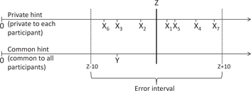
Public hint Y drawn from the interval[Z−10,Z+10] In addition to this private hint X, in each period, you and the other members of your group receive a public hint Y about the unknown number Z. This public hint is also randomly selected over the interval [Z−10,Z+10]. The probability of being selected is the same for any number within this interval. This public hint Y is the same for all participants.

Distinction between private hint X and public hint Y Note that at the first stage, your private hint X and the public hint Y have the same precision: each is drawn from the same error interval. The sole distinction between the two hints is that each participant sees a private hint X that is different from that of the other participants whereas all the participants see the same public hint Y.

How to make a decision? As you do not know the errors associated with your hints, it is natural to choose, as a decision, a number that is between your private hint X and the public hint Y. To make your decisions, you are asked to select two numbers, by clicking on a scale that is defined between your private hint X and the public hint Y. You thus have to choose how to combine your two hints in order to maximize the payoff associated with your decision 1 and your decision 2.

Once you have chosen each of your decisions 1 and 2, click on the Validate button. Once all the participants have done the same, a period ends and you are told the result of the period. Then a new period starts.

As soon as the 10 periods of the first stage are over, the second stage of the experiment begins.

C – Your hints about Z during stage 2 (10 periods)

The second stage is different from the first in that the precision of the public hint increases: it is twice as informative as the private hint about the unknown number Z.

Private hint X drawn from the interval [Z−10, Z+10] In each period, each participant receives a private hint X about the unknown number Z. The private hints are selected randomly from the error interval [Z−10, Z+10]. The probability of being selected is the same for all numbers within this interval. Your private hint and the private hint of all other participants are selected independently from one another from the same interval, so that in general each participant receives a private hint that is different from that of the other participants.
Public hint Y drawn from the interval [Z−5, Z+5] In addition to this private hint X, in each period, you receive a public hint Y about the unknown number Z. This public hint is randomly selected from the interval [Z−5, Z+5]. The probability of being selected is the same for all numbers within this interval. This public hint is the same for all participants.

In each period, as in stage 1, you have to make two decisions. The only difference from the first stage is that the public hint is twice as precise as the private hint.

As soon as the 10 periods of the second stage are over, the third stage of the experiment begins.

D – Your hints about Z during stage 3 (10 periods)

In each period of the third stage, you will receive two hints about Z for making your decisions. This time, the public hint will be less precise: it will be two times less precise than your private hint about the unknown number Z.

Private hint X drawn from the interval [Z−10, Z+10] In each period, each participant receives a private hint X about the unknown number Z. The private hints are selected randomly from the error interval [Z−10, Z+10]. The probability of being selected is the same for all numbers within this interval. Your private hint and the private hint of all other participants are selected independently from one another over the same interval, so that in general each participant receives a private hint that is different from that of the other participants.
Public hint Y drawn from the interval [Z−20, Z+20] In addition to this private hint X, in each period, you receive a public hint Y about the unknown number Z. This public hint is randomly selected from the interval [Z−20, Z+20]. The probability of being selected is the same for all numbers within this interval. This public hint is the same for all participants.

In each period, as in stages 1 and 2, you have to make two decisions. The only difference to the first stage is that the public hint is two times less precise than the private hint.

As soon as the 10 periods of the third stage are over, the experiment ends.

You will be told about each change in stage.

Questionnaires

At the beginning of the experiment, you are asked to fill in an understanding questionnaire on the computer; when all the participants have responded properly, the experiment can begins. At the end of the experiment, you are asked to fill in a personal computer survey. All information will remain confidential.

Payoffs At the end of the experiment, the ECUs you have obtained are converted into euros and paid in cash. 700 ECUs correspond to 1 euros.

Thanks for taking part in the experiment!

C Understanding questionnaire

The training questionnaire varied according to the treatments. Each of the 10 following questions had to be answered by right or wrong, yes or no or multiple choices.

During each period of the three stages of the experiment, you always interact with the same participants.
At each period of the three stages, all the participants of the same group receive the same private hint X.
At each period of the three stages, all the participants receive the same public hint Y.
Is it rational to make a decision outside the interval defined by your two hints?
Your payoff associated with decision 1 does not depend on the average decision 1 of the other members of your group.
To maximize your payoff associated with your decision 2, it is more important that your decision 2 is closer to the unknown number Z than the average decision 2 of the other members of your group.
Suppose the value of Z is equal to 143 and the average decision 2 of the other participants of your group is equal to 133, what will be your payoff in ECU if your decision 2 is equal to 138: 150? 300? 350?
Generally the private hint X is as informative on the average decision 2 of the other participants as the public hint Y.
The difference between stages 1 and 2 is that the public hint Y is more precise than the private hint X on the unknown number Z.
The difference between decision 1 and decision 2 is that the payoff associated with decision 1 is independent from the decision 1 of the other participants whereas the payoff associated with decision 2 depends on the decision 2 of the other participants.

D DExample of decision and feedback screens

E EResults for the decisions in the first period for each group

In each experimental session, subjects were matched into groups of 6 participants. After each period, the feedback screen displayed the history of previous choices. Such a structure may raise the concern that subjects treat the successive games as a repeated game, since they may learn to coordinate with the other participants of their group over periods. To check whether learning issues mattered, we consider in this appendix the weight put on the public signal in the decisions of the first period for each group, instead of the average weight over all periods.

Table 7 presents the first period weight on y in the expectation of the fundamental (decision 1), and Table 8 the first period weight on y in the beauty contest (decision 2).

Table 9 compares the p-values of the statistical tests for the weight on the public signal in decision 1 in the first period and over all periods. Table 10 do the same for the weight in decision 2. The values computed over all periods correspond to the values presented in the text. This appendix shows that statistical results for both the first period and over all periods are very similar.

Table 7:

First period weight on y in the expectation of the fundamental (decision 1).

Sessions	Groups	μη=0		μη=5		μη=20
		ofobs	tfcond	ofobs	tfcond	ofobs	tfcond
1	1	0.45	0.50	0.78	0.90	0.27	0.12
1	2	0.41	0.50	0.77	0.89	0.28	0.09
1	3	0.42	0.50	0.63	0.89	0.27	0.11
2	4	0.58	0.50	0.63	0.90	0.56	0.07
2	5	0.50	0.50	0.68	0.89	0.49	0.07
2	6	0.62	0.50	0.71	0.87	0.28	0.07
3	7	0.50	0.50	0.72	0.89	0.48	0.09
3	8	0.67	0.50	0.83	0.90	0.39	0.18
3	9	0.50	0.50	0.72	0.90	0.31	0.08
4	10	0.38	0.50	0.72	0.90	0.57	0.12
4	11	0.44	0.50	0.72	0.90	0.37	0.08
4	12	0.57	0.50	0.62	0.89	0.34	0.14
5	13	0.45	0.50	0.83	0.91	0.48	0.11
5	14	0.52	0.50	0.72	0.90	0.32	0.08
5	15	0.62	0.50	0.56	0.91	0.37	0.12
6	16	0.48	0.50	0.76	0.89	0.38	0.11
6	17	0.57	0.50	0.62	0.91	0.41	0.08
6	18	0.57	0.50	0.71	0.88	0.31	0.10
Average	1–18	0.51	0.50	0.71	0.90	0.38	0.10
tfuncond	13–18	0.50		0.91		0.09

Table 8:

First period weight on y in the beauty contest (decision 2).

Sessions	Groups	μη=10		μη=5		μη=20
		owobs	twcond	owobs	twcond	owobs	twcond
1	1	0.73	0.87	0.81	0.98	0.55	0.42
1	2	0.70	0.87	0.77	0.98	0.53	0.40
1	3	0.85	0.87	0.93	0.98	0.84	0.41
2	4	0.62	0.87	0.82	0.98	0.56	0.38
2	5	0.76	0.87	0.94	0.98	0.80	0.38
2	6	0.73	0.87	0.88	0.98	0.78	0.38
3	7	0.65	0.87	0.83	0.98	0.55	0.40
3	8	0.82	0.87	0.88	0.98	0.82	0.46
3	9	0.68	0.87	0.88	0.98	0.57	0.39
4	10	0.77	0.87	0.78	0.98	0.62	0.42
4	11	0.65	0.87	0.85	0.98	0.62	0.39
4	12	0.63	0.87	0.73	0.98	0.45	0.43
Average	1–12	0.72	0.87	0.84	0.98	0.64	0.41
twuncond	1–12	0.87		0.99		0.39
5	13	0.74	0.67	0.81	0.95	0.53	0.18
5	14	0.73	0.67	0.75	0.95	0.57	0.15
5	15	0.57	0.67	0.65	0.95	0.46	0.19
6	16	0.68	0.67	0.78	0.94	0.40	0.18
6	17	0.73	0.67	0.75	0.95	0.45	0.16
6	18	0.70	0.67	0.81	0.94	0.50	0.17
Average	13–18	0.69	0.67	0.76	0.95	0.48	0.17
twuncond	13–18	0.67		0.95		0.16

Table 9:

Test results for decision 1.

Hypothesis	Test	1st period	All periods
Treatment order	Wilcoxon rank sum test
Obs. weight is not	G1–6 vs. 7–12, μη=10	p=0.8089	p=0.6859
influenced by	G1–6 vs. 7–12, μη=5	p=0.4624	p=0.1481
treatment order	G1–6 vs. 7–12, μη=20	p=0.1720	p=0.2963
Deviation from theory	Wilcoxon rank sum test
Obs. weight is not	G1–18 vs. theory, μη=10	p=0.7638	p=0.1270
different from	G1–18 vs. theory, μη=5	p=0.0000	p=0.0000
theoretical weight	G1–18 vs. theory, μη=20	p=0.0000	p=0.0000
Signal precision	Wilcoxon matched-pairs signed-rank test
Obs. weight is not	G1–18, μη=10 vs. 5	p=0.0004	p=0.0002
influenced by	G1–18, μη=10 vs. 20	p=0.0023	p=0.0002
precision	G1–18, μη=5 vs. 20	p=0.0002	p=0.0002
Strategic complement.	Wilcoxon rank sum test
Obs. weight is not	G1–6 vs. 13–18, μη=10	p=0.3760	p=0.4184
influenced by degree	G1–6 vs. 13–18, μη=5	p=1.0000	p=0.6304
of strategic complement.	G1–6 vs. 13–18, μη=20	p=0.2963	p=0.3350

Table 10:

Test results for decision 2.

Hypothesis	Test	1st period	All periods
Treatment order	Wilcoxon rank sum test
Obs. weight is not	G1–6 vs. 7–12, μη=10	p=0.5738	p=0.8726
influenced by	G1–6 vs. 7–12, μη=5	p=0.5725	p=0.7475
treatment order	G1–6 vs. 7–12, μη=20	p=0.7479	p=0.1269
Deviation from theory	Wilcoxon rank sum test
Obs. weight is not	G1–12 vs. theory, μη=10	p=0.0000	p=0.0002
different from	G1–12 vs. theory, μη=5	p=0.0000	p=0.000
theoretical weight	G1–12 vs. theory, μη=20	p=0.0000	p=0.0000
	G13–18 vs. theory, μη=10	p=0.0489	p=0.9241
	G13–18 vs. theory, μη=5	p=0.0029	p=0.0025
	G13–18 vs. theory, μη=20	p=0.0051	p=0.0049
Overreaction to theory	Wilcoxon rank sum test
Obs. weight is not	G1–12, μη=10	p=0.0000	p=0.0000
different from	G1–12, μη=5	p=0.1935	p=0.0406
theoretical weight in	G1–12, μη=20	p=0.0000	p=0.0000
1st order expectation	G13–18, μη=10	p=0.0015	p=0.0015
	G13–18, μη=5	p=0.0049	p=0.0048
	G13–18, μη=20	p=0.0028	p=0.0029
Overreaction to obs.	Wilcoxon matched-pairs signed-rank test
Obs. weight is not	G1–12, μη=10	p=0.0025	p=0.0025
different from	G1–12, μη=5	p=0.0038	p=0.0025
obs. weight in	G1–12, μη=20	p=0.0038	p=0.0025
1st order expectation	G13–18, μη=10	p=0.0591	p=0.0360
	G13–18, μη=5	p=0.0935	p=0.0739
	G13–18, μη=20	p=0.0360	p=0.0360
Signal precision	Wilcoxon matched-pairs signed-rank test
Obs. weight is not	G1–12, μη=10 vs. 5	p=0.0025	p=0.0025
influenced by	G1–12, μη=10 vs. 20	p=0.0234	p=0.0025
precision	G1–12, μη=5 vs. 20	p=0.0025	p=0.0025
	G13–18, μη=10 vs. 5	p=0.0355	p=0.0360
	G13–18, μη=10 vs. 20	p=0.0360	p=0.0360
	G13–18, μη=5 vs. 20	p=0.0360	p=0.0360
Strategic complement.	Wilcoxon rank sum test
Obs. weight is not	G1–6 vs. 13–18, μη=10	p=0.4142	p=0.0771
influenced by degree	G1–6 vs. 13–18, μη=5	p=0.0292	p=0.0063
of strategic complement.	G1–6 vs. 13–18, μη=20	p=0.0247	p=0.0081

F Comparison between decisions 1 and 2 and between weights in decisions 2 when r=0.5 and r=0.85

Figure 2:

Average weight assigned to the public signal in decision 1 f (first-order expectation) and in decision 2 w (beauty contest).

G Relative frequency of weights on the public signal in decisions 1 and 2

Figure 3:

Relative frequency of weight assigned to the public signal in decision 1 (first-order expectation); dashed line: uncond. optimal weight; solid line: observed average.

Figure 4:

Relative frequency of weight assigned to the public signal in decision 2 (the action); dashed line: uncond. optimal weight; solid line: observed average.

Figure 5:

Relative frequency of weight assigned to the public signal in decision 2 (the action); dashed line: uncond. optimal weight; solid line: observed average.

H Payoff incentives

Figure 6 represents the expected payoff as a function of deviation from the optimal weight conditional on signals. It shows that deviating from the optimal weight is more costly when μη=20 than when μη=5. According to payoff incentives, one would expect subjects to deviate less from optimal weight with a less precise signal than with a more precise one. The opposite is observed, as described in Sections 4.1.2 and 4.3.2. The observed first-order expectation of the fundamental deviates more from the theory when the public signal is less precise.

Figure 6:

Expected payoff as function of deviation from optimal weight.

References

Ackert, L., B. Church, and A. Gillette. 2004. “Immediate Disclosure or Secrecy? The Release of Information in Experimental Asset Markets.” Financial Markets, Institutions and Instruments 13 (5):219–43.10.1111/j.0963-8008.2004.00077.xSuche in Google Scholar

Alfarano, S., A. Morone, and E. Camacho. 2011. The role of public and private information in a laboratory financial market. Working Papers Serie AD 2011–06, Instituto Valenciano de Investigaciones Econmicas, S.A. (Ivie).Suche in Google Scholar

Amato, J., S. Morris, and H. S. Shin. 2002. “Communication and Monetary Policy.” Oxford Review of Economic Policy 18 (4):495–503.10.1093/oxrep/18.4.495Suche in Google Scholar

Angeletos, G.-M., and A. Pavan. 2004. “Transparency of Information and Coordination in Economies with Investment Complementarities.” American Economic Review (Papers and Proceedings) 94 (2):91–8.10.3386/w10391Suche in Google Scholar

Baeriswyl, R., and C. Cornand. 2010. “The Signaling Role of Policy Actions.” Journal of Monetary Economics 57 (6):682–95.10.1016/j.jmoneco.2010.06.001Suche in Google Scholar

Baeriswyl, R., and C. Cornand. 2014. “Reducing Overreaction to Central Banks Disclosure: Theory and Experiment.” Journal of the European Economic Association 12 (4):1087–126.10.2139/ssrn.1981979Suche in Google Scholar

Cabrales, A., R. Nagel, and R. Armenter. 2007. “Equilibrium Selection through Incomplete Information in Coordination Games: An Experimental Study.” Experimental Economics 10 (3):221–34.10.1007/s10683-007-9183-zSuche in Google Scholar

Cornand, C. 2006. “Speculative Attack and Informational Structure: An Experimental Study.” Review of International Economics 14:797–817.10.1111/j.1467-9396.2006.00608.xSuche in Google Scholar

Cornand, C., and F. Heinemann. 2014. “Measuring Agents’ Reaction to Private and Public Information in Games with Strategic Complementarities.” Experimental Economics 17 (1):61–77.10.1007/s10683-013-9357-9Suche in Google Scholar

Dale, D. J., and J. Morgan. 2012. “Experiments on the Social Value of Public Information.” Mimeo.Suche in Google Scholar

Fischbacher, U. 2007. “Z-tree: Zurich Toolbox for Ready-Made Economic Experiments.” Experimental Economics 10 (2):171–8.10.1007/s10683-006-9159-4Suche in Google Scholar

Heinemann, F., R. Nagel, and P. Ockenfels. 2004. “The Theory of Global Games on Test: Experimental Analysis of Coordination Games with Public and Private Information.” Econometrica 72 (5):1583–99.10.1111/j.1468-0262.2004.00544.xSuche in Google Scholar

Heinemann, F., R. Nagel, and P. Ockenfels. 2009. “Measuring Strategic Uncertainty in Coordination Games.” Review of Economic Studies 76:181–221.10.1111/j.1467-937X.2008.00512.xSuche in Google Scholar

Hellwig, C., and L. Veldkamp. 2009. “Knowing What Others Know: Coordination Motives in Information Acquisition.” Review of Economic Studies 76:223–51.10.1111/j.1467-937X.2008.00515.xSuche in Google Scholar

Middeldorp, M., and S. Rosenkranz. 2011. “Central Bank Transparency and the Crowding Out of Private Information in an Experimental Asset Market.” Federal Reserve Bank of New York Staff Reports (487).10.2139/ssrn.1782850Suche in Google Scholar

Morris, S., and H. S. Shin. 2002. “Social Value of Public Information.” American Economic Review 92 (5):1521–34.10.1257/000282802762024610Suche in Google Scholar

Nagel, R. 1995. “Unraveling in Guessing Games: An Experimental Study.” American Economic Review 85:1313–26.Suche in Google Scholar

Shapiro, D., X. Shi, and A. Zillante. 2014. “Level-k Reasoning in a Generalized Beauty Contest.” Games and Economic Behavior 86:308–29.10.1016/j.geb.2014.04.002Suche in Google Scholar

Stahl, D. O., and P. W. Wilson. 1994. “Experimental Evidence on Players’ Models of Other Players.” Journal of Economic Behavior and Organization 25:309–27.10.1016/0167-2681(94)90103-1Suche in Google Scholar

Published Online: 2015-12-3

Published in Print: 2016-1-1

Artikel in diesem Heft

https://doi.org/10.1515/bejte-2015-0002

Schlagwörter für diesen Artikel

heterogeneous information; beauty contest; experiment; public information