Estimating Expected Asset Returns with the Present Value Model of Consumption and Fed Forecasts

1 Introduction

In recent years, significant attention has been given to the connection between the macroeconomy and financial markets. One prominent model utilized to establish this link is the present value model of consumption. This model utilizes the idea that the present discounted value of consumption equals the present discounted value of lifetime wealth. An implication of this relationship is that an equilibrium relationship between consumption and wealth provides us with information about agents’ expectations of future movements in consumption and wealth. One of the challenges in empirical implementation of present value model of consumption is that human wealth is unobservable. The conventional approach in the literature is to proxy human wealth with current labor income. Whelan (2008) presented a framework where the assumption about unobservable human wealth is not required. According to that framework, the present value model can be expressed as follows:

In this equation, x _t is excess consumption that represents the logarithm of consumption minus labor income, a _t represents the logarithm of observable household assets, r t a represents the return on these assets, and ρ is a known constant slightly less than one. The model suggests that the logarithmic ratio of excess consumption (consumption exceeding labor income) to observable assets can be expressed as an expected discounted sum of future returns on household assets minus future growth rates of excess consumption. Therefore, an unexpected increase in excess consumption today implies either news of higher future returns or a downward revision in expected future growth rates of excess consumption. Previous studies, including Whelan (2008) and Lettau and Ludvigson (2001), have adopted the approach of using the excess consumption-assets ratio and the consumption-wealth ratio as indicators for future asset returns and future excess consumption growth rates.^[1] Lettau and Ludvigson (2001, 2005 specifically employ the estimated residuals from a cointegrating regression of consumption, labor income, and wealth (cay) as a proxy for expected asset returns. These studies have provided evidence suggesting that households adjust their consumption spending in anticipation of changes in the return on household assets. This has the implication that asset returns can be predicted based on the consumption decision of the households.

In this paper, we present an alternative approach to estimating expected asset growth. We utilize Greenbook^[2] forecasts of excess consumption growth (Δx _t+j ) on the right hand side of the present value model and estimate expected asset growth as a residual. Greenbook forecasts are prepared by the Fed Board Staff and are presented to the Federal Open Market Committee (FOMC) prior to each of their meetings. In particular, our approach yields the following formula for expected asset growth:

This approach offers several advantages. The existing approach in the literature estimates the present discounted value of asset returns and excess consumption growth jointly and attributes most of the variations in this combined series to movements in expected asset return. Our approach of using the Greenbook forecasts of expected excess consumption growth clearly separates these two unobserved variables and estimates expected asset growth as a residual from the above equation. Another key advantage is that our approach gets around the problem of model uncertainty. Currently, there is no consensus on whether the VAR or State Space approach is superior for estimating expected excess consumption growth or asset return. By incorporating Greenbook forecasts, we mitigate this uncertainty. Additionally, our approach addresses the challenge of estimation uncertainty. As shown in this paper, these forecasts exhibit strong predictive capabilities for future excess consumption growth. Leveraging sophisticated models, Greenbook forecasts effectively aggregate information about future movements in excess consumption growth. Numerous studies in the forecasting literature have highlighted the value of these forecasts in providing insights into macroeconomic variables.^[3] By adopting this alternative approach and leveraging Greenbook forecasts, our research contributes to enhancing the understanding and prediction of asset growth with a present value model.

Our findings indicate that when Greenbook forecasts are used as a proxy for expected excess consumption growth in the present value model, the expected asset returns obtained as residuals do not possess informative content about future movements in asset returns. This contrasts with previous literature that has demonstrated the predictive usefulness of present value models for future returns. To explore the possibility that Greenbook forecasts may include measurement errors in household expectations of expected excess consumption growth, we also estimate a model assuming classical measurement error in Greenbook forecasts. Under this framework, the residual from the present value model represents the expected asset return and an error term. However, the results from this analysis are remarkably similar to those obtained without considering measurement error.

2 Data Description

We use data at quarterly frequency and our sample runs from 1978 through 2017. Data on household assets come from the Federal Reserve Board’s Flow of Funds, with durable goods expenses subtracted to measure consumption. The study adopts Whelan (2008) and Lettau and Ludvigson (2001) methodologies for calculating after tax labor income. The data is deflated using the personal consumption expenditure price index.

To proxy expected consumption growth and income growth, we rely on the Greenbook forecasts. These forecasts become publicly available with a delay of five years. Therefore, our sample is limited to data spanning the years 1978–2017. The information regarding Greenbooks can be obtained from the Federal Reserve Bank of Philadelphia.^[4] We specifically utilize 1–4 quarter ahead forecasts for consumption and real disposable income growth.^[5]

Table 1 illustrates the effectiveness of Greenbook forecasts in predicting consumption and income growth across various forecast horizons, demonstrating the Greenbook forecasts’ predictive capability for future trends in both consumption and income growth. The findings are derived from a regression analysis of observed consumption growth and income growth against forecasts at differing horizons. As anticipated, the R ² values are highest for current quarter forecasts and decrease for longer horizons. Nonetheless, the coefficients for the forecasts remain significant at all conventional levels across various horizons. These regression outcomes indicate that Greenbook forecasts are forward-looking and not adversely affected by model and estimation uncertainties. Figure 1 compares the observed levels of excess consumption with forecasts for different horizons. The level forecasts are imputed from the growth forecasts with the past observed level of consumption and after tax labor income.

Figure 1:

Actual excess consumption and Greenbook forecasts at different horizons.

3 Model Specification

3.1 A Present Value Model of Consumption

This section is based on the present value model proposed by Whelan (2008) and Campbell and Shiller (1988) as a baseline model. Whelan (2008) examines a budget constraint that depicts the dynamics of total observable assets that can be expressed as follows:

(3) A t + 1 = R t + 1 a ( A t + Y t − C t )

where A _t is total household assets, R t + 1 a is the gross return on assets, Y _t is labor income and C _t is consumption. Dividing across by A _t and taking logs we get:

(4) Δ a t + 1 = r t + 1 a + log 1 − C t − Y t A t

Define, excess consumption as X _t = C _t − Y _t .

Solving the above equations and rearranging, yields the following expression:

(5) x t − a t ≈ ρ r t + 1 a + κ − Δ x t + 1 + ρ ( x t + 1 − a t + 1 )

Solving forward via repeated substitution and imposing the condition that lim _j→∞ ρ ^−j (x _t+j − a _t+j ) = 0 and taking conditional expectation at time t, we obtain:

(6) x t − a t ≈ ρ κ 1 − ρ + E t ∑ j = 1 ∞ ρ j r t + j a − Δ x t + j

We can write the present discounted value of the expected asset returns as E t ∑ j = 1 ∞ ρ j r t + j a ≈ x t − a t + E t ∑ j = 1 ∞ ρ j Δ x t + j . We proxy the expected excess consumption growth with the forecasts calculated from Greenbook. The discount factor ρ = 1 − exp ( x ̄ − a ̄ ) is estimated to be 0.971. Expected consumption growth beyond 4-quarters is approximated by 4-quarter ahead forecasts. In particular, we obtain expected asset growth with the following formula:

(7) E t ∑ j = 1 ∞ ρ j r t + j a ≈ x t − a t + ρ E r Δ x t + 1 G B + ρ 2 E r Δ x t + 2 G B + ρ 3 E r Δ x t + 3 G B + ρ 4 E r Δ x t + 4 G B + ρ 4 1 − ρ E r Δ x t + 4 G B

The estimated expected asset returns for this exercise, shown in Figure 2, are plotted alongside observed asset returns. Table 2 presents the cross-correlation between these estimated returns and realized returns at various horizons. Notably, the contemporaneous correlation is 0.27, impressive considering the noisiness in quarterly asset returns. The correlation with excess consumption-asset ratio is lower, at 0.08. However, when examining the correlation with future realized returns, the expected measure underperforms, becoming insignificant after two quarters. Yet, the correlation with the excess consumption-asset ratio remains significant up to six quarters. The results are also similar for the correlation between expected returns and the discounted sum of realized returns over the next four quarters, ∑ j = 1 4 ρ j r t + j a .

Figure 2:

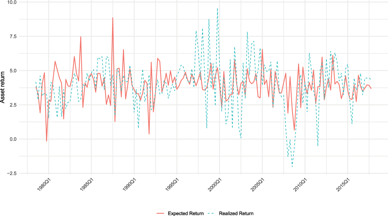
Expected return from a present-value model with Greenbook forecasts.

Table 2:

Cross lag correlation with realized asset returns.

Lags	r t e	x t − a t
Panel A: Cross lag correlation with quarterly return
0	0.27	0.08
1	0.16	0.20
2	0.08	0.19
3	0.08	0.16
4	−0.03	0.19
6	−0.02	0.15
9	−0.05	0.10
12	−0.06	0.03
Panel B: Cross lag correlation with one-year ahead return
0	0.14	0.31
1	0.11	0.26
2	0.16	0.25
3	0.11	0.24
4	0.11	0.23
6	0.06	0.17
9	0.03	0.07
12	−0.01	−0.01

1. The table shows correlation between expected asset return ( r t e ) and excess consumption asset ratio (x _t − a _t ) with realized asset returns at different horizons.

To test whether the current ratio indeed predicts future asset movements and consumption growth, we performed a Granger causality test. This tests whether past expected returns predict future realized returns after accounting for lags in realized returns. As reported in Table 3, we found no evidence that past expected returns Granger-cause future realized returns. On the contrary, past realized returns seem to predict expected returns, challenging the efficacy of present value models in predicting asset returns. Additionally, we found no support for the hypothesis that past movements in the excess consumption-asset ratio Granger-cause future realized returns. However, there is strong evidence that this ratio predicts forecasts of excess consumption growth at various horizons, as detailed in Table 3.

Table 3:

Granger causality test results.

H 0	p-Value
r t e Granger causes r t	0.37
r t Granger causes r t e	0.00
r t e Granger causes r t_4	0.28
r t_4 Granger causes r t e	0.00
r t e , m Granger causes r t	0.67
r t Granger causes r t e , m	0.00

1. r t e is expected asset return from the baseline GB forecast model. r _t is realized asset r _{t_4} represents one year ahead return. r t e , m is expected return from measurement error model.

Table 4 reports our in-sample predictive regression results. As anticipated, past realized returns, explaining only 5 % of future returns, are not a significant predictor. Moreover, past expected returns, accounting for just 1.1 % of future returns, also show limited predictive power. Including both lagged realized and expected returns as regressors does not improve the R ², which remains at 5 %, and the individual coefficients continue to be insignificant. Overall, the results suggest that expected asset returns obtained through the present value model do not provide valuable insights into future asset returns.

Table 4:

Predictive ability test for expected asset return.

Predictive regression for realized asset returns (r t )
Explanatory variable	Model 1	Model 2	Model 3
Lagged r t	0.24		0.22
	(0.11)		(0.15)
Lagged r t e		0.20	0.11
		(0.14)	(0.41)
R 2	0.05	0.01	0.05

1. p-Values are shown in parentheses. The dependent variable is realized asset return (r _t ). r t e is expected return from our baseline model.

3.2 Greenbook Forecasts as Imperfect Proxies for Household’s Expected Return

It is reasonable to consider that the expected asset returns of households may differ from those forecasted by Federal Reserve staff members. One reason could be that Fed staff have access to a superior information set. However, Faust, Swanson, and Wright (2004) suggest that any advantage in the Federal Reserve Board’s information set, not publicly shared, is likely minor and subtle. They note that the information from Federal Reserve policy surprises about the economy’s state does not consistently enhance the forecasts based on their statistical releases. This indicates that the superiority of Greenbook forecasts may not be due to asymmetric information alone, but rather due to the staff’s enhanced ability to aggregate available information.

Recognizing the minimal differences in the information set, in this study, we hypothesize that the expected asset returns, estimated as the residual from the present value relationship, could be prone to measurement errors. Suppose E t ∑ j = 1 ∞ ρ j Δ x t + j = ∑ j = 1 ∞ ρ j Δ x t + j G B + u t , u t ˜ i i d N 0 , σ u 2 . We assume that household’s expected excess consumption growth equals Greenbook forecasts plus a serially uncorrelated measurement error. This implies that

(8) x t − a t + ∑ j = 1 ∞ ρ j Δ x t + j G B = E t ∑ j = 1 ∞ ρ j r t + j a + u t .

The above equation has two unobservables on the right hand side. To identify these two unobservables, we assume that expected presented discounted value of asset returns follow an AR(1) process. In particular, the model has the following structure

(9) E t ∑ j = 1 ∞ ρ j r t + j a = r a , t e = α + β r a , t − 1 e + ε t , ε t ˜ i i d N 0 , σ ε 2

We assume that measurement error u _t , and the shock to expected asset returns, ɛ _t are uncorrelated, i.e. cov(u _t , ɛ _t ) = 0. The above two equations can be cast into a state space form and estimated using maximum likelihood via the Kalman filter. The estimated expected asset returns are reported in Figure 3. The figure plots the estimated asset returns from this exercise with the one from the model that does not assume any measurement error. It is clear that the filtering of expected asset return does not change the results obtained from the previous section. The correlation between expected return from the Greenbook forecasts (baseline) and the one obtained with the measurement error model is 0.99. Expected return obtained from the measurement error model is slightly less volatile as expected. However, all other properties like Granger causality and cross lag correlation remains similar.

Figure 3:

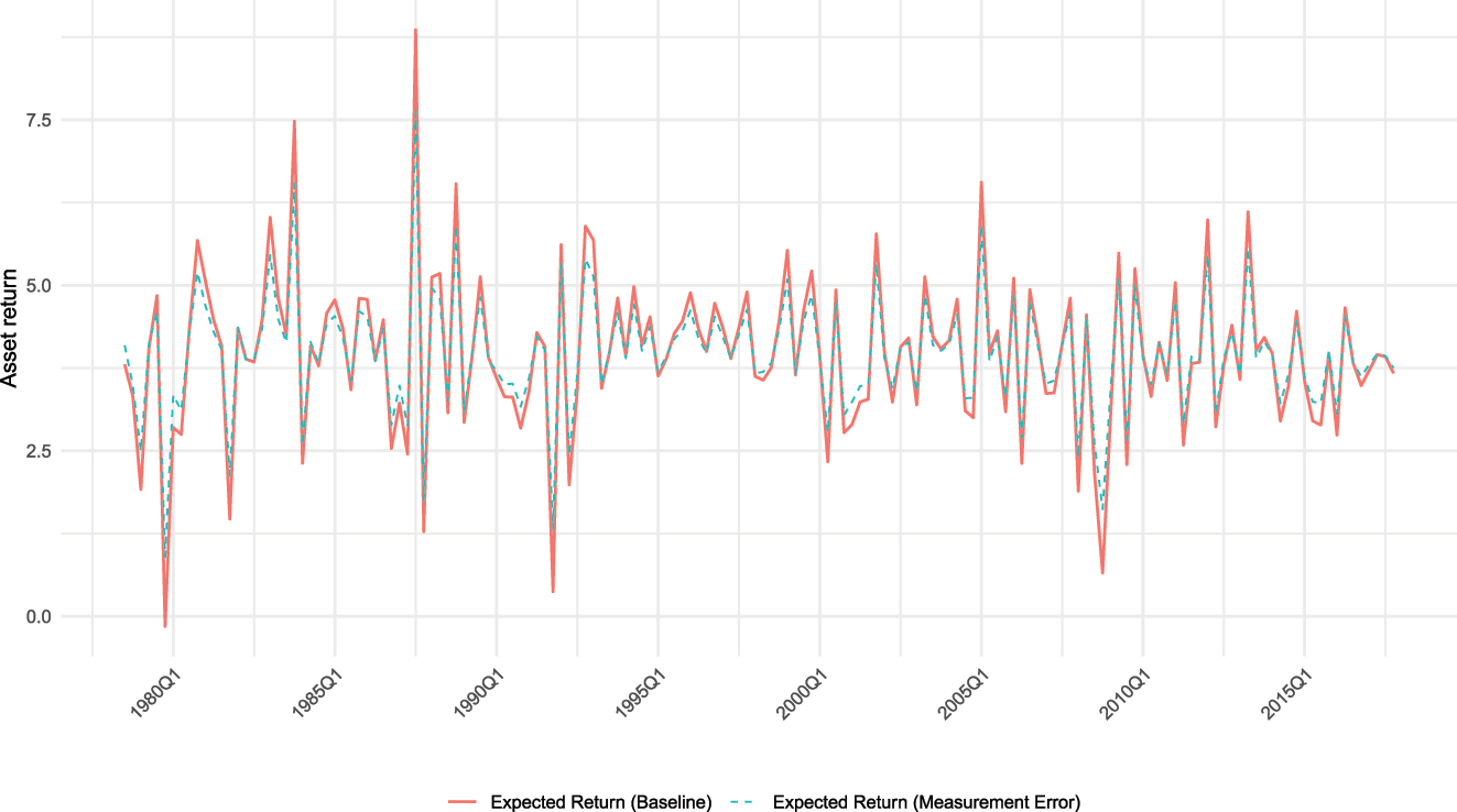
Comparison with a measurement error model.

4 Conclusions

This paper utilizes the data provided by the Greenbook forecasts of consumption and income to derive expected asset returns using a present value model of consumption. The rationale behind this approach is the recognition that Greenbook forecasts possess significant information regarding future changes in consumption and income, and they are not subject to the limitations of conventional modeling choices faced by researchers. By employing this methodology, the paper calculates expected asset returns as a residual value from the present value model of consumption. Utilizing observable excess consumption-asset ratios and approximating expected excess consumption growth with Greenbook forecasts enabled the extraction of expected asset growth in the United States from 1978 to 2017. The findings indicate that the expected asset returns obtained through this approach do not provide valuable insights into future asset returns, contradicting some existing literature that suggests asset returns can be predicted using a present value model of consumption.

References

Bhatt, V., N. Kundan Kishor, and H. Marfatia. 2020. “Estimating Excess Sensitivity and Habit Persistence in Consumption Using Greenbook Forecasts.” Oxford Bulletin of Economics & Statistics 82 (2): 257–84. https://doi.org/10.1111/obes.12333.Search in Google Scholar
Bidarkota, P. V., and B. V. Dupoyet. 2007. “The Impact of Fat Tails on Equilibrium Rates of Return and Term Premia.” Journal of Economic Dynamics and Control 31 (3): 887–905. https://doi.org/10.1016/j.jedc.2006.03.001.Search in Google Scholar
Brandt, M. W., and Q. Kang. 2004. “On the Relation between the Conditional Mean and Volatility of Stock Returns: A Latent VAR Approach.” Journal of Financial Economics 72: 217–57. https://doi.org/10.1016/j.jfineco.2002.06.001.Search in Google Scholar
Campbell, J. Y., and R. J. Shiller. 1988. “The Dividend-Price Ratio and Expectations of Future Dividends and Discount Factors.” Review of Financial Studies 1: 195–277. https://doi.org/10.1093/rfs/1.3.195.Search in Google Scholar
Conrad, J., and G. Kaul. 1988. “Time-Variation in Expected Returns.” Journal of Business 61: 409–25. https://doi.org/10.1086/296441.Search in Google Scholar
Faust, Jon, Eric T. Swanson, and Jonathan H. Wright. 2004. “Do Federal Reserve Policy Surprises Reveal Superior Information about the Economy?” Contributions to Macroeconomics 4 (1): 10. https://doi.org/10.2202/1534-6005.1246.Search in Google Scholar
Kishor, N. K. 2010. The Superiority of Greenbook Forecasts and the Role of Recessions. National Bank of Poland Working Paper, (74).10.2139/ssrn.1744017Search in Google Scholar
Kishor, N. K., and S. Kumari. 2015. “Consumption and Expected Asset Returns: An Unobserved-Component Approach.” Macroeconomic Dynamics 19 (5): 1023–44. https://doi.org/10.1017/s1365100513000680.Search in Google Scholar
Lettau, Martin, and Sydney Ludvigson. 2001. “Consumption, Aggregate Wealth, and Expected Stock Returns.” The Journal of Finance 56: 815–49. https://doi.org/10.1111/0022-1082.00347.Search in Google Scholar
Lettau, Martin, and Sydney Ludvigson. 2005. “Expected Returns and Expected Dividend Growth.” Journal of Financial Economics 76: 583–626. https://doi.org/10.1016/j.jfineco.2004.05.008.Search in Google Scholar
Pastor, L., and R. F. Stambaugh. 2006. Predictive Systems: Living with Imperfect Predictors. Working Paper University of Chicago and CRSP.10.3386/w12814Search in Google Scholar
Romer, Christina, and David Romer. 2000. “Federal Reserve Information and the Behavior of Interest Rates.” The American Economic Review 90: 429–57. https://doi.org/10.1257/aer.90.3.429.Search in Google Scholar
Rytchkov, O. 2007. Filtering Out Expected Dividends and Expected Returns. Unpublished Paper. Texas A&M.Search in Google Scholar
Sims, C. A. 2002. “Solving Linear Rational Expectations Models.” Computational Economics 20 (1–2): 1.Search in Google Scholar
Van Binsbergen, J. H., and R. S. Koijen. 2010. “Predictive Regressions: A Present‐Value Approach.” The Journal of Finance 65 (4): 1439–71.10.1111/j.1540-6261.2010.01575.xSearch in Google Scholar
Whelan, Karl. 2008. “Consumption and Expected Asset Returns without Assumptions about Unobservables.” Journal of Monetary Economics 55 (7): 1209–21. https://doi.org/10.1016/j.jmoneco.2008.08.006.Search in Google Scholar
© 2024 Walter de Gruyter GmbH, Berlin/Boston
Articles in the same Issue
- Frontmatter
- Advances
- Corporate Tax Rates, Allocative Efficiency, and Aggregate Productivity
- Contributions
- Endogenous Financial Friction and Growth
- Decomposing Structural Change
- Industry Impacts of US Unconventional Monetary Policy
- Monetary Policy Transmission in Canada – A High Frequency Identification Approach
- Child Labor, Corruption, and Development
- Inflation Uncertainty from Firms’ Perspective, Overconfidence and Credibility of Monetary Policy
- Does Nominal Wage Stickiness Affect Fiscal Multiplier in a Two-Agent New Keynesian Model?
- To Create or to Redistribute? That is the Question